Study on Sloshing Characteristics in a Liquid Cargo Tank under Combination Excitation

Abstract

Sloshing is a common flow phenomenon in liquid cargo tanks and has a great negative impact on the stability and safety of ship navigation. It is important to understand the sloshing process of tanks under the excitation of complex external conditions for the transportation of liquid cargo. In this paper, the sloshing characteristics of a liquid cargo tank are studied under the combination excitation conditions of roll and surge. The pressure distribution characteristics at different positions of the cargo tank are discussed, along with the influence of different excitation conditions on the pressure of the cargo tank. The results show that under the condition of combination excitation, the fluid sloshes along the diagonal direction of the tank, and the peak liquid height and peak pressure are located on the diagonal corner of the tank. The peak pressure at the lowest point on the diagonal of the tank is proportional to the amplitude of the roll angle and surge, and the change in roll angle amplitude has a significant impact on the pressure and liquid height at different positions.

1. Introduction

With the continuous and in-depth implementation of international marine environmental protection, liquefied natural gas (LNG) fuel has become increasingly used due to its high efficiency and cleanliness. When an LNG carrier encounters adverse sea conditions, the excitation of waves causes the mass center and free surface of the LNG in the cargo hold to deviate from the original equilibrium state, resulting in sloshing. A strong impact on the bulkhead structure when the ship encounters intense sloshing results in property losses and casualties. However, LNG carriers in actual navigation encounter more complex excitations (roll and surge) than single excitations (roll or surge). Therefore, the study of the sloshing behavior and anti-sloshing design under the combination excitation is significant for the navigation safety of LNG carriers.

In terms of theoretical research, Moiseev [1] proposed a nonlinear sloshing theory based on potential flow theory using the asymptotic and modal methods. Faltinsen et al. [2] used the boundary element method to predict the nonlinear sloshing model of a rectangular tank under resonance excitation conditions. In another study, Faltinsen et al. [3] used the modal analysis method to study the two-dimensional liquid sloshing process in a circular tank. Budiansky [4] theoretically calculated the natural modes and frequencies of circular tubes and spherical tanks at different liquid loading heights.

In terms of experimental research, Kim et al. [5] visualized the sloshing process using a high-speed camera and discussed the causes of pressure measurement errors in the sloshing experiment from both macroscopic and microscopic aspects. Trimulyono et al. [6] evaluated the equivalent damping coefficient of an FPSO model storage tank under roll excitation at different loading rates. The results showed that ship damping is inversely proportional to the loading rate and the amplitude of the roll angle. Yu et al. [7] studied the sloshing mitigation characteristics of vertical grids under different frequency excitation conditions. Akyildiz et al. [8] designed an experimental device for sloshing to study the pressure distribution characteristics at different positions in the tank and the three-dimensional effect caused by sloshing. Zou et al. [9] conducted a sloshing model experiment of viscous liquid to study the influence of liquid viscosity on sloshing. The results show that viscous friction has a certain dissipation effect on the sloshing pressure. Doh et al. [10] used a panoramic particle image velocimetry (PIV) system to conduct experimental research on the sloshing characteristics in the LNG ship cargo tank model. The results showed that the oscillation amplitude has a large impact on the horizontal velocity of the liquid.

The numerical simulation of sloshing can be further divided into the finite difference method (FDM) [11], the finite element method (FEM) [12], the finite volume element method (FVM) [13], the boundary element method (BEM) [14] and the smooth particle dynamics method (SPH) [15]. Considering the influence of the turbulence model on the numerical simulation results of sloshing, Liu et al. [16] used the large eddy simulation method (LES) and the Smagorinsky subgrid scale (SGS) to simulate the turbulence effect and verified the accuracy of the model with experimental data. Tang et al. [17] used STAR-CCM+ software to numerically simulate the sloshing process in the tank. The results showed that adjusting the value of the gradient parameter k in the k-ε model can make the sloshing waveform in the tank more realistic. In terms of free surface capture, the volume of fluid (VOF) free surface capture algorithm has been used for sloshing numerical simulation research. For example, Borg et al. [18] studied the sloshing characteristics of fluid in a rectangular box with a chamfer and the sloshing reduction characteristics of the baffled tank under different loading rates. Hoch et al. [19] studied the sloshing behavior of liquid in a storage tank. The results showed that the VOF method better describes the change in the liquid level, but the predicted sloshing impact pressure is lower than the experimental measurement. Based on the OpenFOAM simulation platform, Xue et al. [20] numerically simulated the anti-sloshing characteristics of porous media materials in cylindrical tanks. In addition, some scholars have used the level-set method to capture sloshing free surfaces. For example, Xin et al. [21] used the three-dimensional gradient-augmented level set (GALS) two-phase flow model to capture the sloshing nonlinear free surface. The results showed that the numerical simulation is in good agreement with the experiment.

In summary, the relevant theoretical analysis and research on liquid sloshing characteristics in holding tanks have been relatively developed, but there are also some limitations. For example, when the sloshing in the tank is intense and there are obvious liquid level breaking and attacking phenomena, the theoretical analysis solution is no longer applicable. Although numerical simulation studies can obtain more comprehensive flow information of the flow field in the tank, the simulation results still need to be compared and verified with experiments. Furthermore, in the existing studies, for both numerical simulation and experimental research, scholars mostly focus on the sloshing characteristics of tanks under a single degree of freedom, while the ship navigation process is mostly multi-degree-of-freedom complex motion under the action of wind and waves. Therefore, it is necessary to study the sloshing characteristics of liquid tanks under combination excitation involving multiple degrees of freedom.

In this paper, the sloshing process of fluid in a cargo tank under the combination excitation of roll and surge is the research object. Through numerical simulation and experimental verification methods, the trend of the sloshing liquid level under combination excitation is clarified, and the impact pressure distribution of the bulkhead under combined excitation is explored. The research conclusions obtained in this paper provide theoretical support for tank structure design and anti-sloshing design under combination excitation.

2. Numerical Model and Experimental Platform

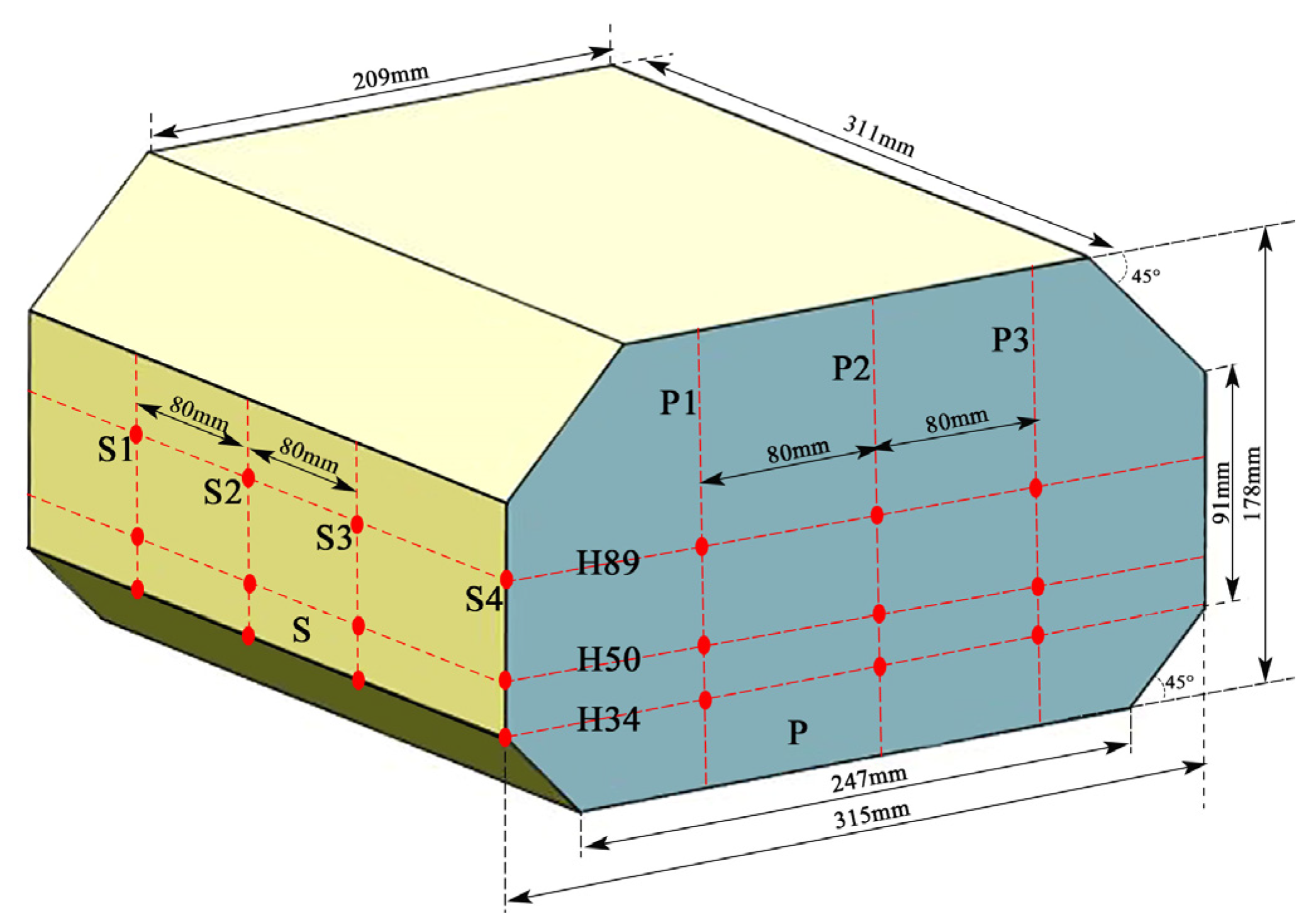
2.1. Geometric Model

Figure 1 shows the geometric model of the cargo tank studied in this paper. The model is a membrane-type cargo tank, commonly used in LNG carriers and proportionally reduced to laboratory scale. The size of the real cargo tank is 15.75 m × 15.55 m × 8.9 m (width × length × height) at a scale of 1:50. The model size is 0.315 m × 0.311 m × 0.178 m (width × length × height). The data monitoring points in the numerical simulation are selected as the intersection points of the vertical lines and the horizontal lines as shown in Figure 1. Among them, vertical lines P2 and S2 are located at the geometric centers of the two sidewalls, while S4 is located at the edge of the geometric model, and straight lines H89, H50 and H34 are horizontal lines with heights of 89 mm, 50 mm and 34 mm, respectively. Monitoring points were named, for example, P1H50, which represents the intersection of the vertical line P1 and the horizontal line at a height of 50 mm.

2.2. Numerical Model

The dynamic mesh method in the open source CFD tool OpenFOAM was adopted to solve the Navier-Stokes and other transport equations under the combination excitation. The surfaces of the tank are the wall boundaries. The Navier-Stokes equation was solved by the PISO method, and the turbulence model adopted the standard k-Ꜫ model. The Courant number was set to 0.2, and the time step was adaptively adjusted. The second-order schemes Gauss vanLeer and Crank Nicolson were used for the spatial and time discretization, respectively. Hydrostatic pressure and zero velocity initialized the flow field. In all the cases of sloshing, the values of α_l and α_g were both 0.5.

2.2.1. Volume Fraction Equation

The primary focus of this paper is on gas–liquid two-phase flow, in which the liquid phase is water and the gas phase is air. The interface between the two phases can be obtained by solving the continuity equation of the volume fraction. Equation (1) describes the volume fraction equation of the liquid phase as follows:

$$\frac{\partial }{\partial t}\left({\rho }_l{\alpha }_l\right)+\frac{\partial }{\partial x_j}\left({\rho }_l{\alpha }_l{u}_i\right)=0$$

(1)

where the subscripts l and g represent the liquid and gas phases, respectively; $\rho$ is the density; α is the volume fraction; and the volume fraction of the liquid phase and the gas phase are represented by α_l and α_g, respectively. Their relationship is shown in Equation (2) as follows:

$${\alpha }_l+{\alpha }_g=1$$

(2)

2.2.2. Momentum Equation

In the VOF model, the entire computational domain shares a set of momentum equations, and the velocity field obtained by solving is composed of the gas phase and the liquid phase. The momentum equations are shown in Equations (3)–(5) as follows:

$$\frac{\partial (\rho u_i)}{\partial t}+\frac{\partial \left(\rho u_i{u}_j\right)}{\partial x_j}=-\frac{\partial p}{\partial x_i}+\rho g_i+\frac{\partial }{\partial x_j}\left(\mu \frac{\partial u_i}{\partial x_j}-\rho {\overline{{u^{\prime }}_i{u}^{\prime }}}_j\right)+{\overrightarrow{F}}_{{}_{CSF}}$$

(3)

$$\rho ={\alpha }_l{\rho }_l+(1-{\alpha }_l){\rho }_g$$

(4)

$$\mu ={\alpha }_l{\mu }_l+(1-{\alpha }_l){\mu }_g$$

(5)

where $\rho$ is the average density of the fluid in the grid; $\mu$ is the average viscosity of the fluid in the grid; $\overrightarrow{u}$ is the vector velocity; and ${\overrightarrow{F}}_{{}_{CSF}}$ is the surface tension. The continuum surface force (CSF) surface tension model [22] was selected. The CSF surface tension model is shown in Equation (6) as follows:

$${\overrightarrow{F}}_{CSF}={\sigma }_{l.g}\frac{\rho k_l\nabla {\alpha }_l}{\frac{1}{2}\left({\rho }_l+{\rho }_g\right)}$$

(6)

where ${\sigma }_{l,g}$ is the surface tension coefficient between the gas and liquid phases where ${\sigma }_{l,g}={0.071}^{}n/m$; $k$ is the surface curvature at the gas–liquid interface; and $n$ is the surface normal vector of the interface, which is defined in Equation (7) as follows:

$$n=\nabla {\alpha }_l$$

(7)

The surface curvature $k$ at the gas–liquid interface is defined as the divergence of the unit vector $\widehat{n}$ as follows:

$$\widehat{n}=\frac{n}{\left|n\right|}$$

(8)

$$k=\nabla ·\widehat{n}$$

(9)

2.2.3. Transport Equations for the Standard k-ε Model

The turbulence kinetic energy, k, and its rate of dissipation, ε, are obtained from the following transport equations:

$$\frac{\partial }{\partial t}\left(\rho k\right)+\frac{\partial }{\partial x_i}\left(\rho k{u}_i\right)=\frac{\partial }{\partial x_j}\left[\left(\mu +\frac{{\mu }_t}{{\sigma }_k}\right)\frac{\partial k}{\partial x_j}\right]+G_k+G_b-\rho \epsilon -Y_M$$

(10)

$$\frac{\partial }{\partial t}\left(\rho \epsilon \right)+\frac{\partial }{\partial x_i}\left(\rho \epsilon u_i\right)=\frac{\partial }{\partial x_j}\left[\left(\mu +\frac{{\mu }_t}{{\sigma }_{\epsilon }}\right)\frac{\partial \epsilon }{\partial x_j}\right]+C_{1\epsilon }\frac{\epsilon }{k}\left(G_k+C_{3\epsilon }{G}_b\right)-C_{2\epsilon }\rho \frac{{\epsilon }^2}{k}$$

(11)

$${\mu }_t=\rho C_{\mu }\frac{k^2}{\epsilon }$$

(12)

In these equations, G_k represents the generation of turbulence kinetic energy due to the mean velocity gradients, calculated as described in Modeling Turbulent Production in the k-ε Models; G_b is the generation of turbulence kinetic energy due to buoyancy, calculated as described in Effects of Buoyancy on Turbulence in the k-ε models; and Y_M represents the contribution of the fluctuating dilatation in compressible turbulence to the overall dissipation rate, calculated as described in Effects of Compressibility on Turbulence in the k-ε models.

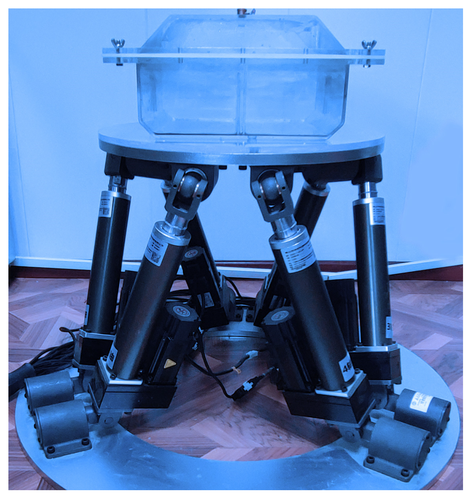
2.3. Six-Degrees-of-Freedom Motion Experimental Platform

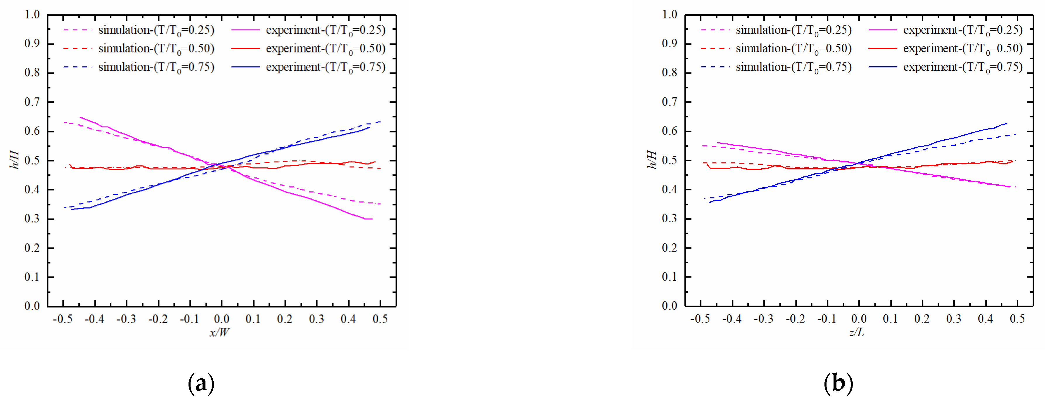
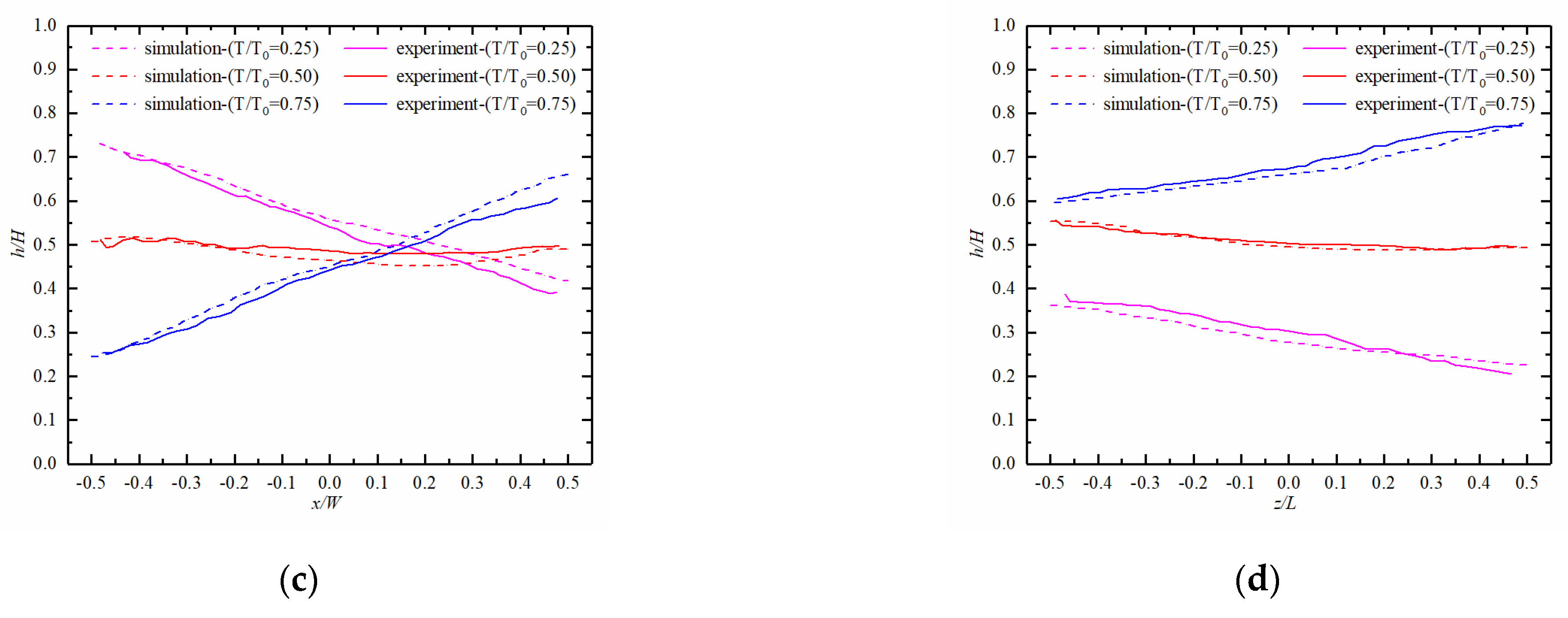
As shown in Figure 2, the six-degrees-of-freedom experimental motion platform built mainly includes a sloshing tank, hydraulic cylinder and a six-degrees-of-freedom motion platform. The sloshing tank was installed above the platform. The motion platform is driven by six hydraulic cylinders controlled by the host to move in six degrees of freedom and further drive the movement of the tank to realize the sloshing of the liquid in the tank. The motion of the experimental platform is shown in Equation (13) as follows [23]:

$$Z=A\cdot sin\left(2\pi f\cdot t\right)$$

(13)

where Z is the response output, A is the motion amplitude, f is the motion frequency, and t is the time. During the experiment, the motion platform was controlled by adjusting the values of A and f. The experimental platform can run continuously for more than 12 h, and the position drift of each hydraulic cylinder meets the requirements of less than 0.00025 m.

3. Model Validation

To verify the accuracy of the numerical simulation method used in this paper, the experimental results and numerical simulation results obtained under the same conditions were compared and analyzed, including qualitative comparisons of the gas-liquid interface profile (as shown in Figure 3) and quantitative comparisons of dimensionless liquid level height variation characteristics (as shown in Figure 4). The selected conditions for validation are shown in

Table 1. Model validation parameter settings.

Type	Roll Angle φ (°)	Surge Amplitude λ (mm)	Frequency f (Hz)	Filling Rate
Roll excitation	10	-	0.58	0.5
Surge excitation	-	50	0.58	0.5
Combination excitation	10	50	0.58	0.5

.

Figure 3 shows that the liquid surface topography obtained from the experiment and simulation under the rolling, surge and combination excitation are consistent. Compared with Figure 4, it can be seen that there is a slight deviation between the numerical simulation results and the experimental data at the position near the wall, which is due to the wall attachment effect of the fluid, but, in general, the numerical simulation is consistent with the experimental curve, which means that the numerical model adopted can describes the sloshing process of the tank exactly.

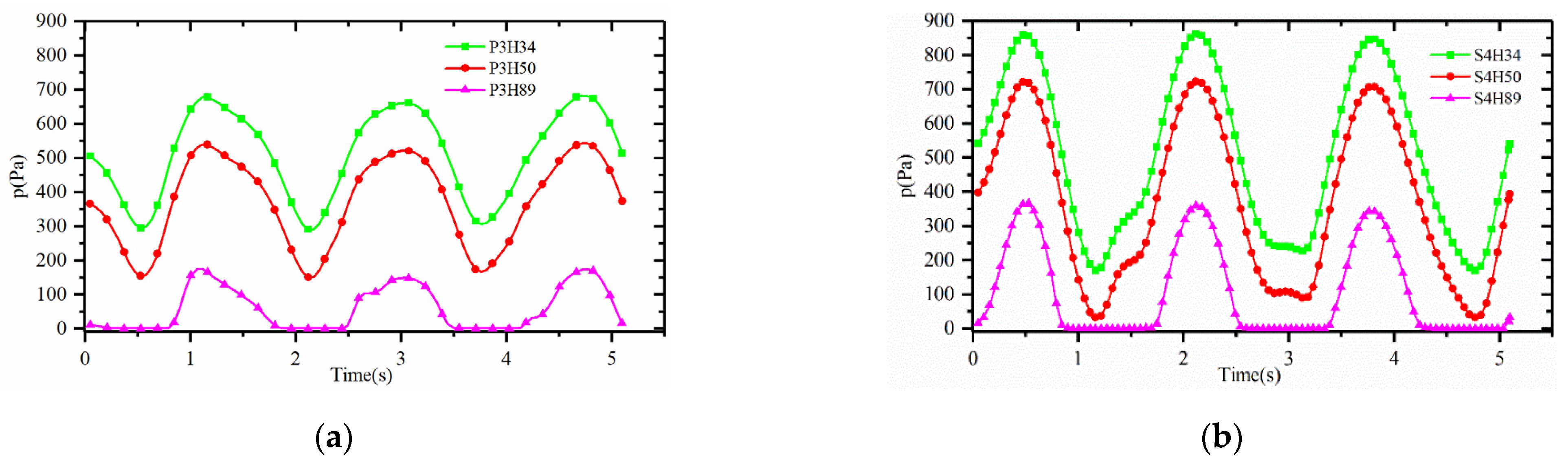
4. Results and Discussion

To study the sloshing behavior of the tank under different excitation conditions, numerical simulations of the tank motion under roll and surge conditions were carried out, and the variation in tank pressure at each monitoring point on the sidewall was analyzed. Then, the numerical simulation of the multiple-degrees-of-freedom sloshing process under the combination excitation of roll and surge was carried out. The pressure variations at different positions are mainly discussed, and the topographic variation characteristics of the liquid surface at different times are quantitatively analyzed. The numerical simulation conditions are as shown in

Table 2. Numerical simulation case settings.

Type	Roll Angle φ (°)	Surge Amplitude λ (mm)	Frequency f (Hz)	Filling Rate
Roll excitation	10	-	0.58	0.5
Surge excitation	-	50	0.58	0.5
Combination excitation	3, 6, 10	30, 40, 50	0.58	0.5

.

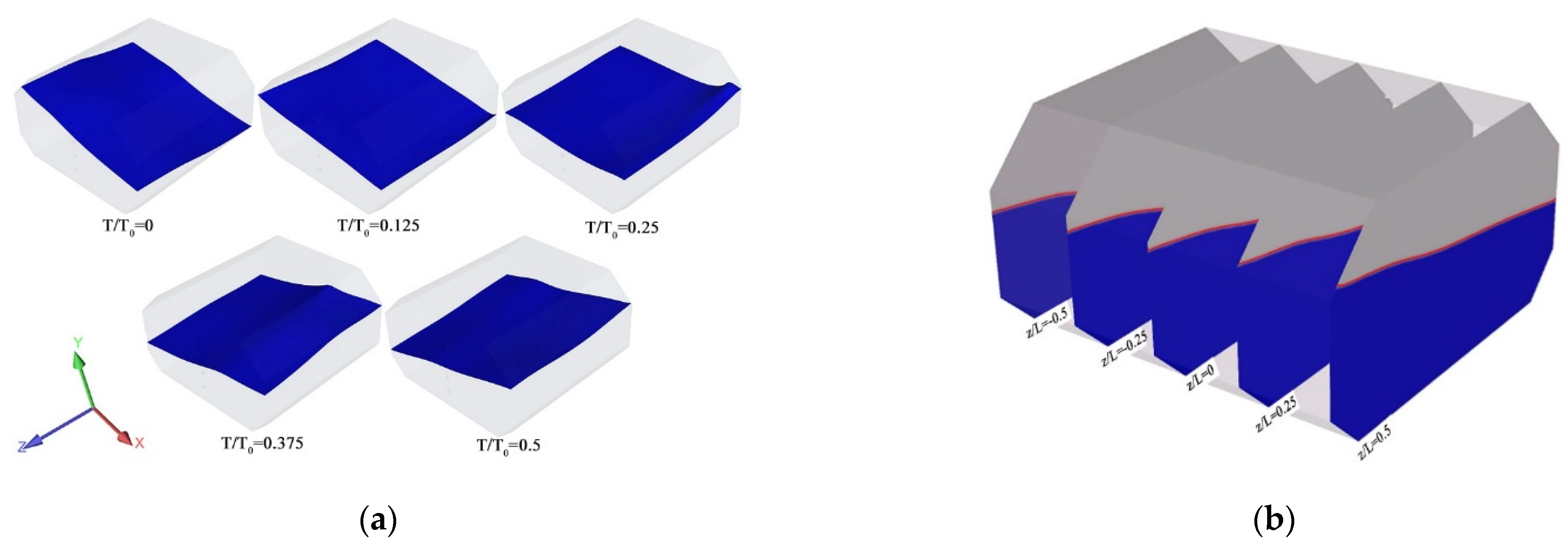
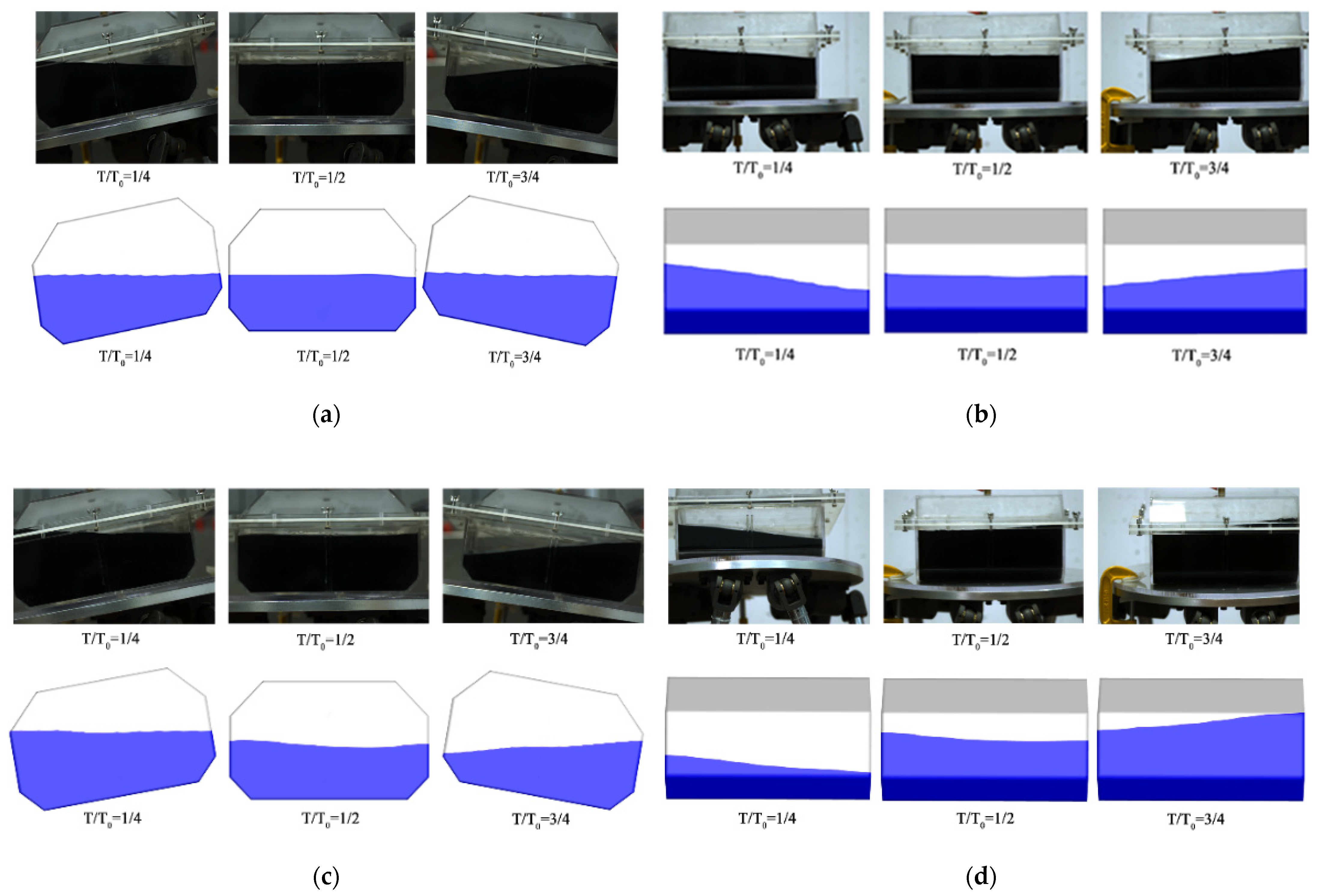
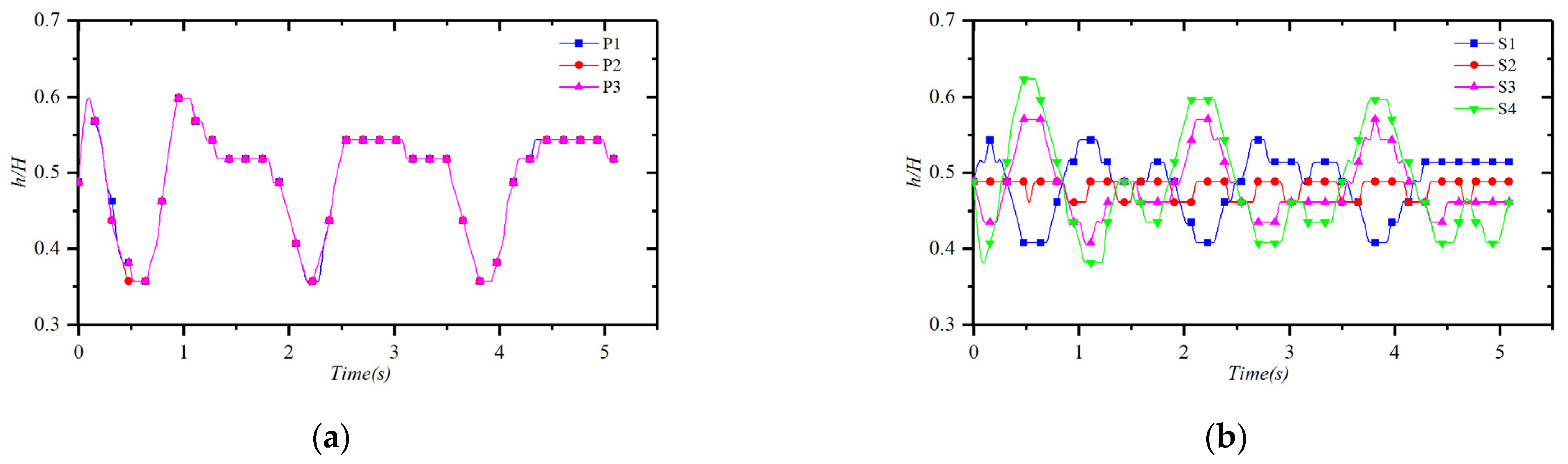
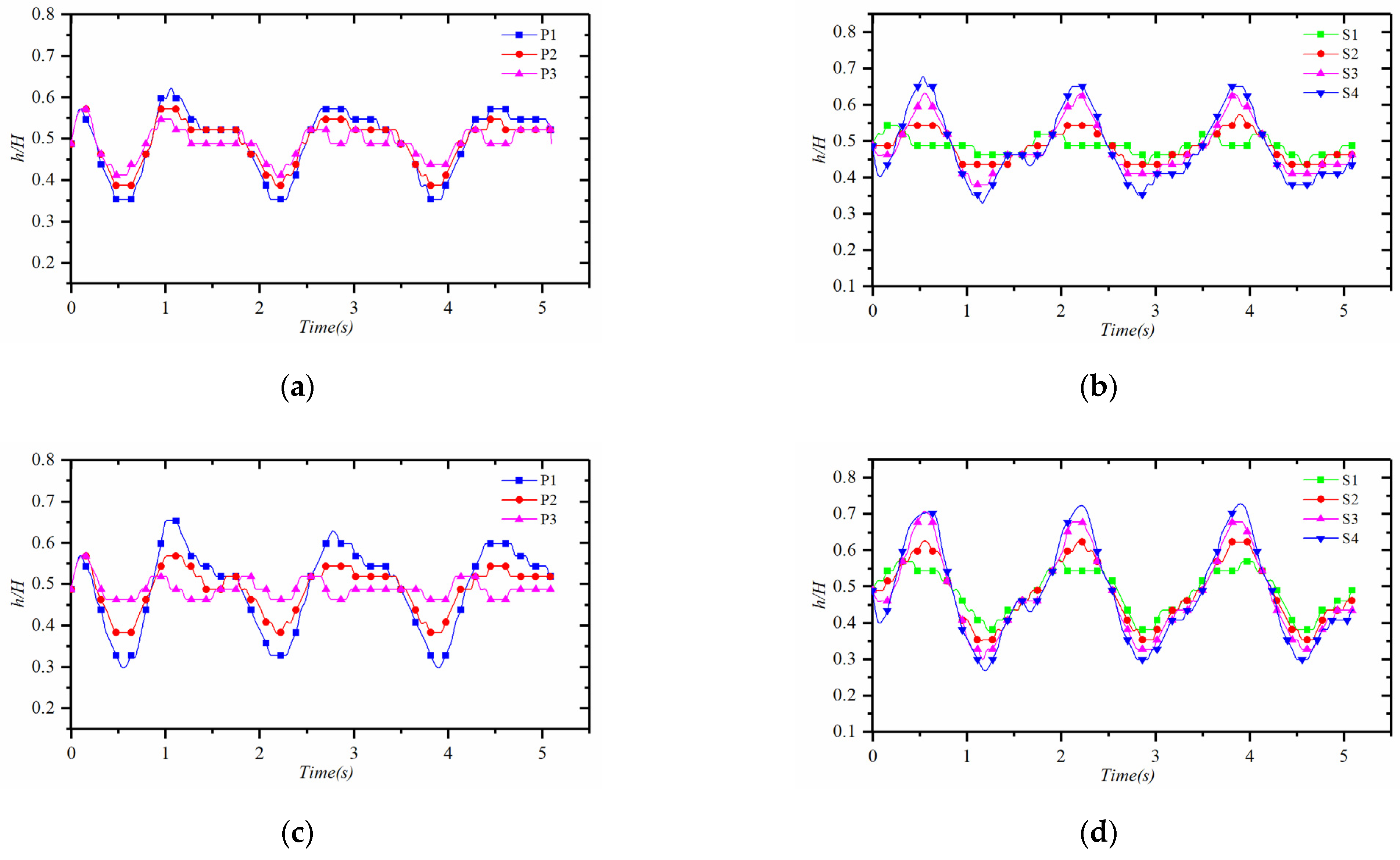
4.1. Liquid Sloshing Characteristics under Roll Excitation

Figure 5 shows the variation of the liquid level on the vertical line at different positions of the tank under the excitation conditions of rolling (f = 0.58 Hz and φ = 10°). The liquid level on the S plane changes more than that on the P plane. The liquid level heights at lines P1 and P3 show periodic changes in the range of 0.25 H, and the two curves have opposite trends, while the liquid level height at the P2 position changes little. The liquid level at S1–S4 also changes periodically, with a similar trend.

Figure 6 shows the pressure distribution at different positions during the roll. Because of the impact of the periodic liquid sloshing on the tank wall, the pressure of each monitoring point changes periodically. At the same height, the pressure of the monitoring point on the S plane is much greater than that on the P plane. Figure 6a,b show that for the monitoring points on the same vertical line and at different levels, the more significant pressure fluctuations are closer to the bottom of the tank. Figure 6c,d show the pressures of monitoring points on the P plane and the S plane at the same height, respectively. Figure 6c shows that the trend of pressure at the monitoring point on the P plane is consistent with the trend of the liquid level in Figure 5a. This is because the pressure changes on the P plane during rolling mainly come from the static pressure change caused by the liquid surface change. Figure 6d shows that the pressures of the monitoring points at the same level on the S plane are the same, and the pressure value is higher than that of the monitoring points at the same level on the P plane. The reason is that under roll excitation, the pressure on the S plane includes not only the static pressure change caused by the change in the liquid level but also the impact dynamic pressure on the S plane.

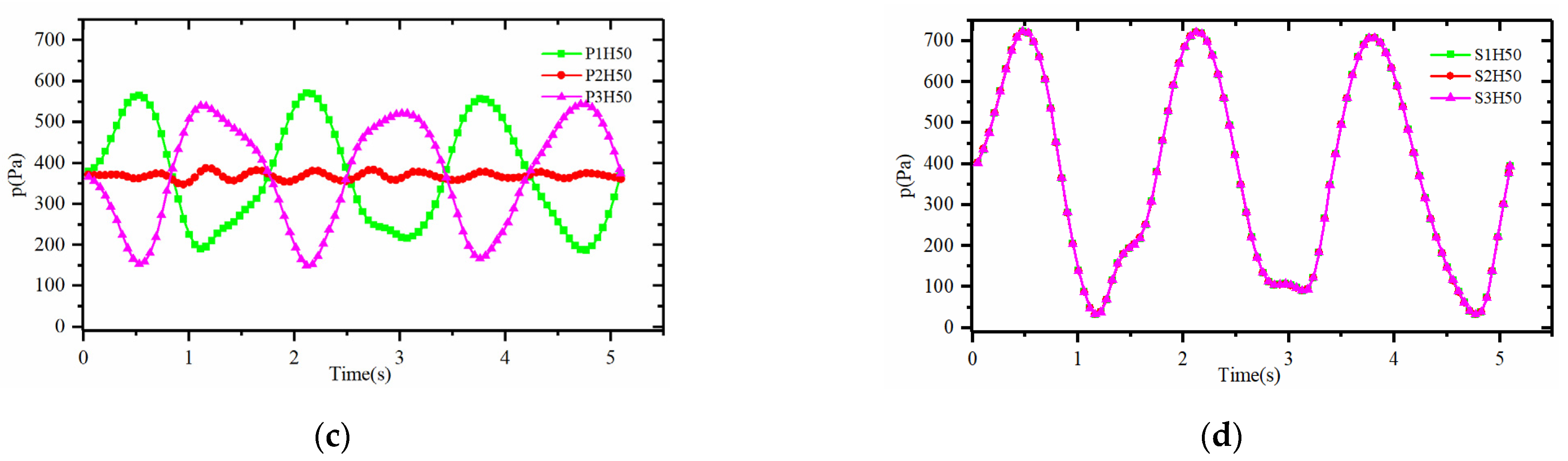
4.2. Liquid Sloshing Characteristics under Surge Excitation

Figure 7 shows the variation of the liquid level on lines P1–3 and S1–4 during the sloshing process of the tank under the condition of surge excitation. It is show that the liquid level on the P plane changes more dramatically than on the S plane, the liquid level changes on lines P1, P2 and P3 are similar, the liquid levels on S1, S2, S3 and S4 are different, the liquid level change of midline S2 is the smallest, and the liquid level change of S4 farther from the midline is the most severe. In addition, the liquid levels on S1 and S3 located at the same distance on both sides of S2 have the same degree of change, but in opposite directions.

Figure 8 shows the pressure distribution of the monitoring points at different positions under the surge condition. Comparing Figure 8a,b, the pressure distribution trends of the monitoring points on lines P2 and S3 are similar, and at higher locations, the pressure of the monitoring points is smaller, and the range of variation is smaller. However, as the liquid surface mainly impacts the P plane during surge excitation, the pressure of monitoring points on P2 is larger than that of S3 in general. Figure 8c shows that the pressure distribution at the monitoring point at a height of 50 mm on the P plane is the same because the liquid level on the P plane is at the same level under surge excitation. Figure 8d shows that during surge excitation, the pressure change at the monitoring point on the P plane is caused by the change in the liquid level and the change in the static pressure at the monitoring point. Therefore, the trend of the pressure at the monitoring point on the P plane is the same as that shown in Figure 7b.

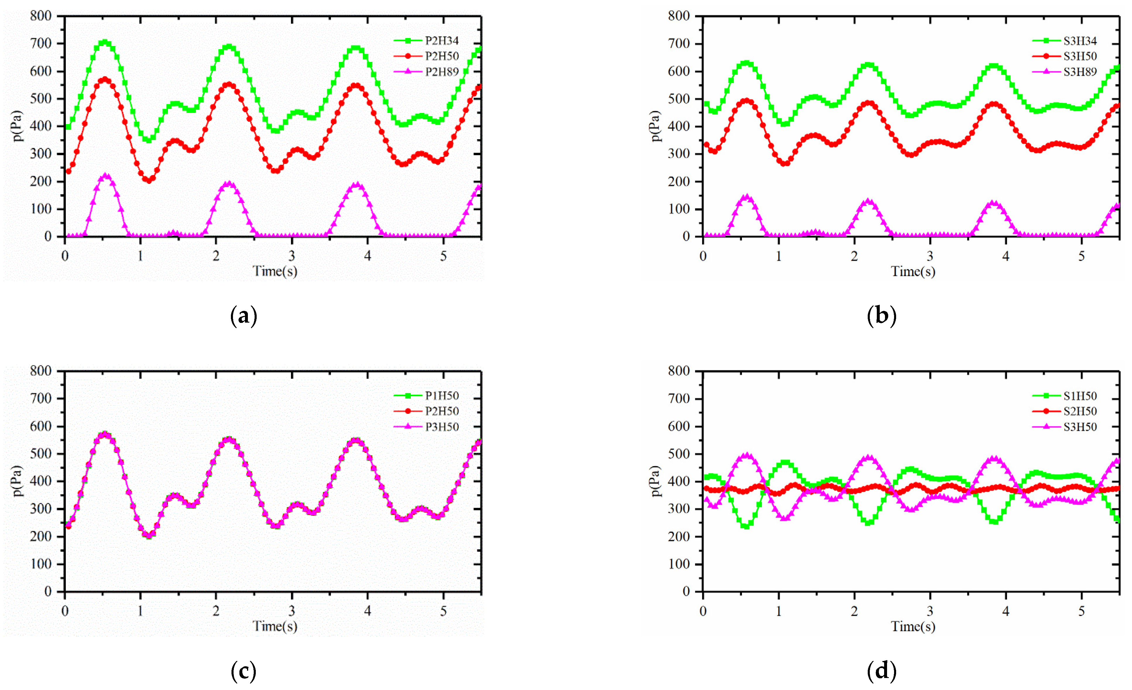
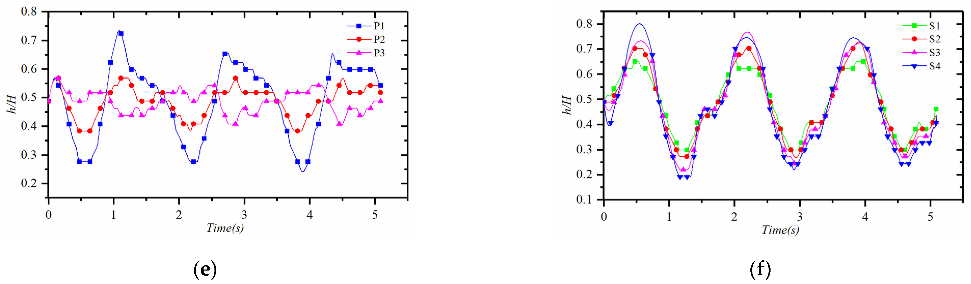
4.3. Liquid Sloshing Characteristics under Combination Excitation

Considering that the excitations of carriers during navigation are mostly combination excitations with multiple degrees of freedom, combination excitation with two degrees of freedom, roll and surge, is studied. The morphological characteristics of the liquid level in the tank and the variation of the liquid level height at different positions are analyzed, and the sloshing behavior under combination excitation conditions is studied.

Figure 9a shows the change in the sloshing liquid surface profile under the combination excitation condition (f = 0.58 Hz, φ = 10°, λ = 50 mm). Compared with the liquid level variation under the single-degree-of-freedom excitation condition, the liquid level variation under the combination excitation condition is more complex and has significant asymmetry; overall, the liquid level changes periodically along the diagonal direction.

To facilitate the observation and analysis of the liquid level change under combination excitation, the cross sections z/L = 0.5, z/L = 0.25, z/L = 0, z/L = −0.25 and z/L = −0.5 were selected as shown in Figure 9b, and the surface profile characteristics at different times were quantitatively analyzed. Figure 10 shows the distribution of the liquid level height on the section at different times. When T/T₀ = 0, the liquid level gradually decreased along the positive x/S and negative z/L directions. The highest point, h/H = 0.85, occurred on section z/L = 0.5, and the lowest point, h/H = 0.19, occurred on section z/L = −0.5. When T/T₀ = 0.125, compared with T/T₀ = 0, the liquid level increased along the positive x/S direction and the negative z/L direction, but the overall distribution is consistent with that at T/T₀ = 0. At the time of T/T₀ = 0.25, the liquid level had a positive movement trend along x/S, and the overall liquid level remained at h/H = 0.5. When T/T₀ = 0.375 and T/T₀ = 0.5, the liquid level gradually increased along the positive x/S direction and the negative z/L direction, and when T/T₀ = 0.5, the maximum positive x/S liquid level was h/H = 0.85.

Figure 11 shows the time-varying characteristic of the liquid level height at different positions. Compared with Figure 5 and Figure 7, the liquid level variation curves at different positions under the combination excitation condition are different, and the peak value of the liquid level height increases. After the sloshing is stable, the closer to P1 on the P plane, the greater the liquid level fluctuation range. The maximum liquid level height at P1 can reach h/H = 0.65, and the closer to S1 on the S plane, the greater the liquid level fluctuation range. The maximum liquid level at S4 is h/H = 0.78.

The time-varying characteristics of pressure at different monitoring points under combination excitation are further discussed below. Figure 12 shows the pressure time-varying curves of different monitoring points. The data in the figure show that under combination excitation, the degree of liquid sloshing is greater, and the sloshing form is more complex than that under the single degree of freedom excitation. The pressure peaks at all monitoring points are increased, and the pressure time-varying curves at some monitoring points are more complex. The data in Figure 12a,c show that due to the influence of hydrostatic pressure, the overall pressure and peak pressure at the monitoring points near the bottom of the tank are larger. Figure 12b,d show that under the condition of combination excitation, the liquid in the tank mainly sloshes along the diagonal direction of the tank. For the monitoring points at the same horizontal height, the closer to line S1 on the P plane, the greater the impact and the greater the pressure value. The pressure value at the monitoring point on centerline S2 on the S plane is the smallest, and the impact and pressure both increase with distance from the centerline. The maximum peak pressure at S4 can reach 900 Pa.

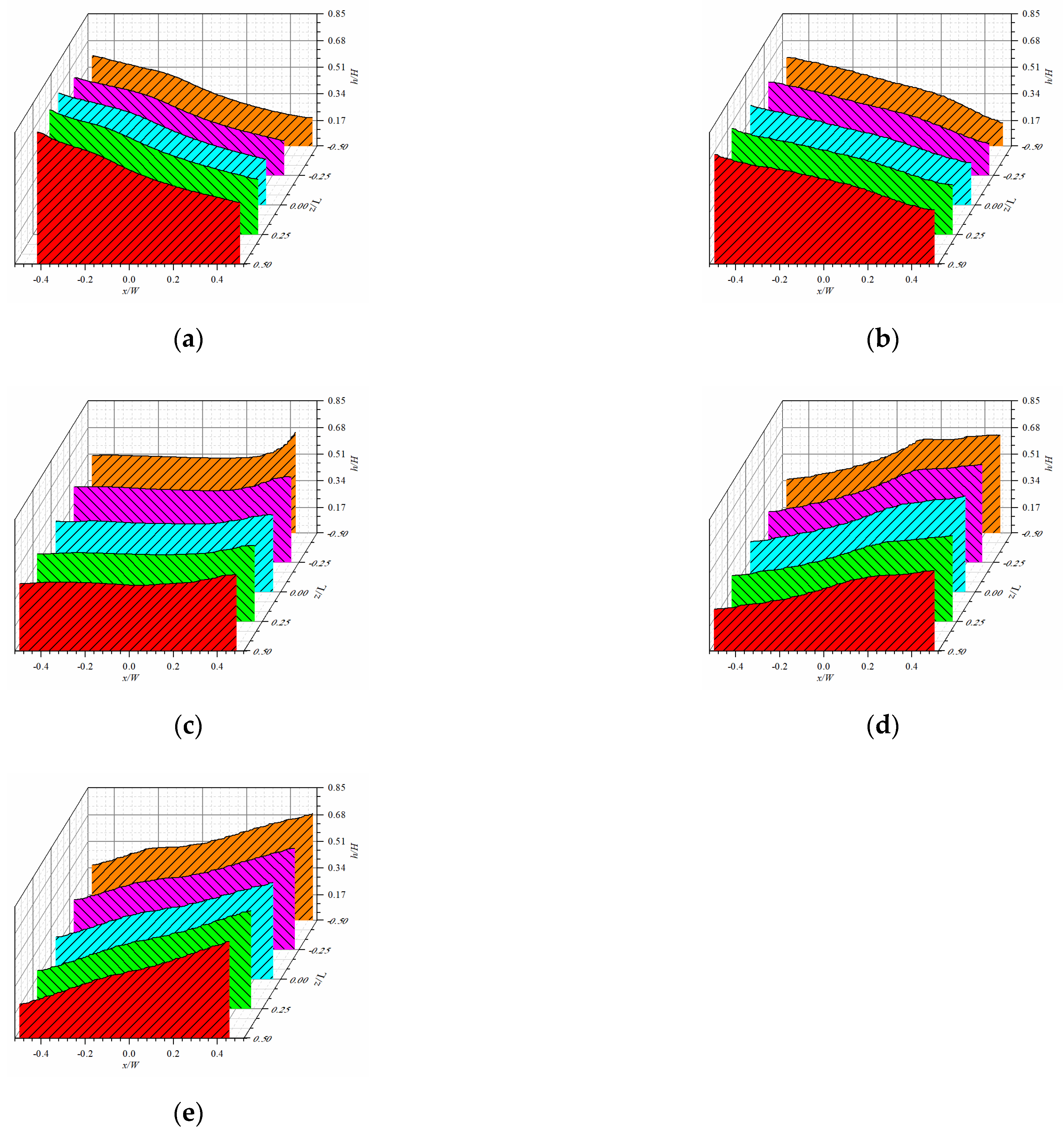
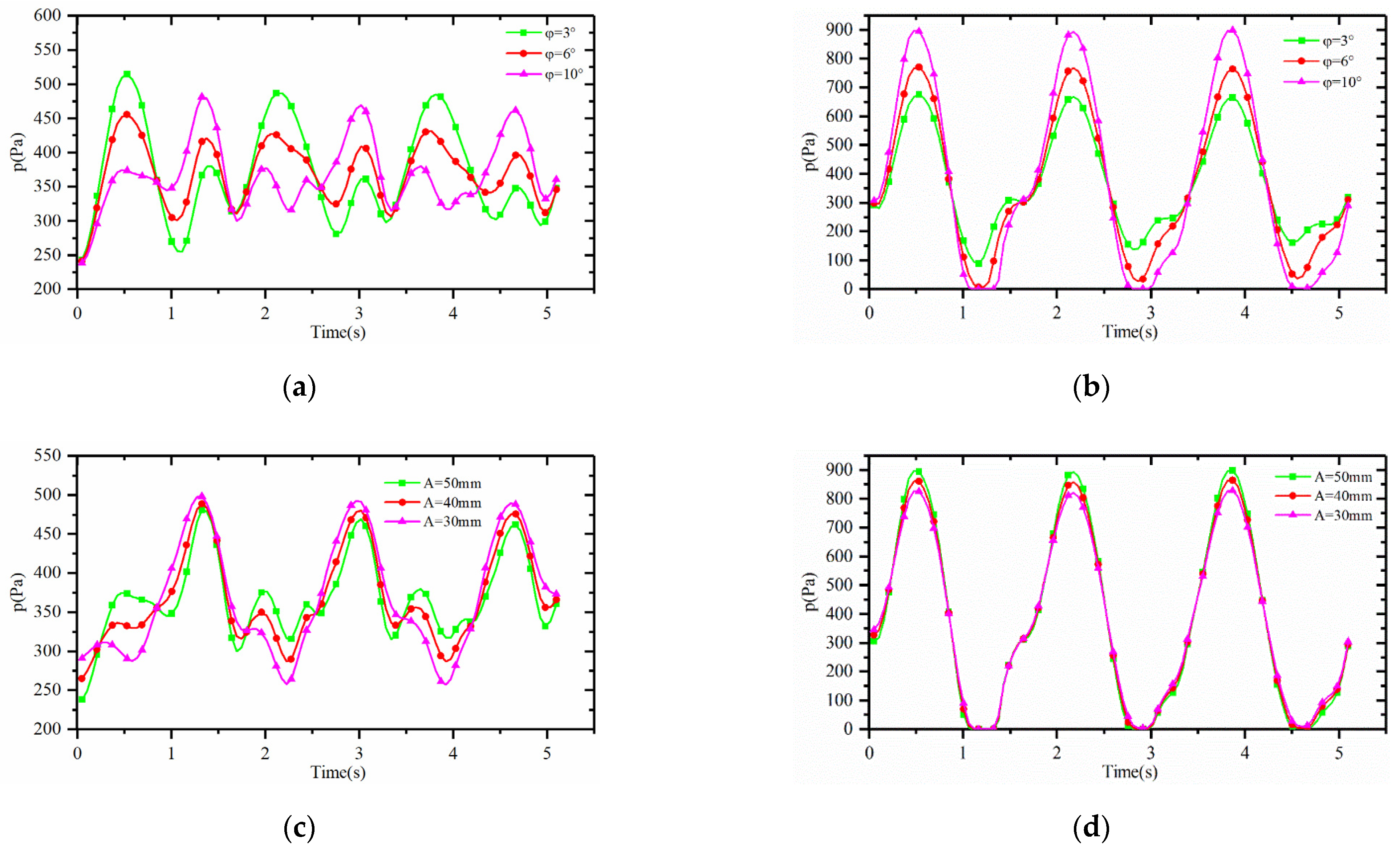
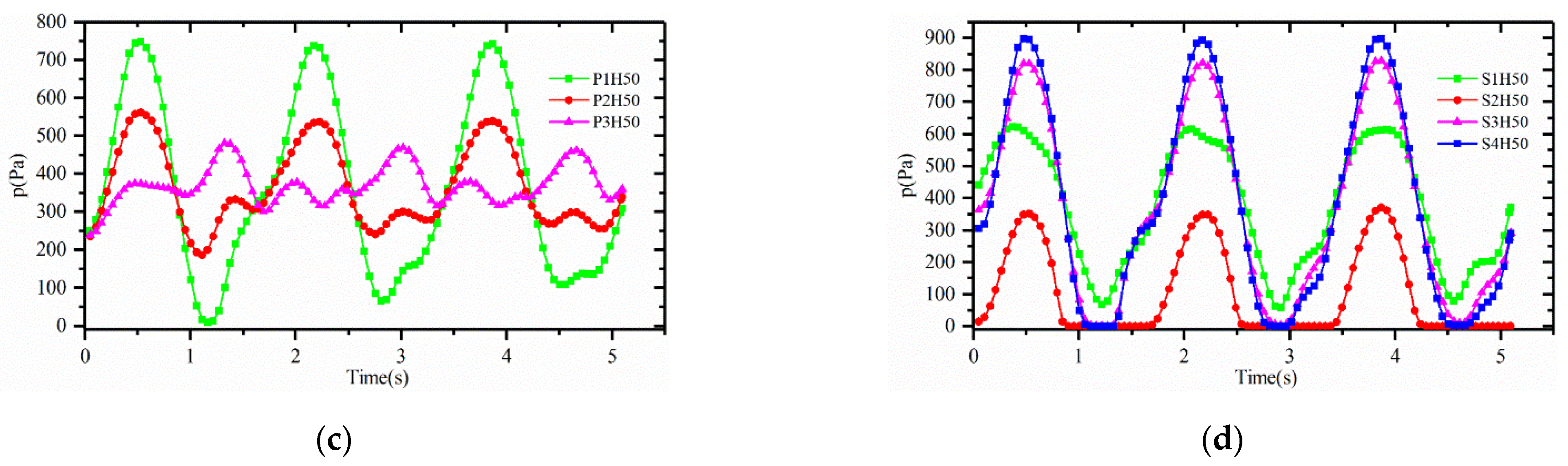
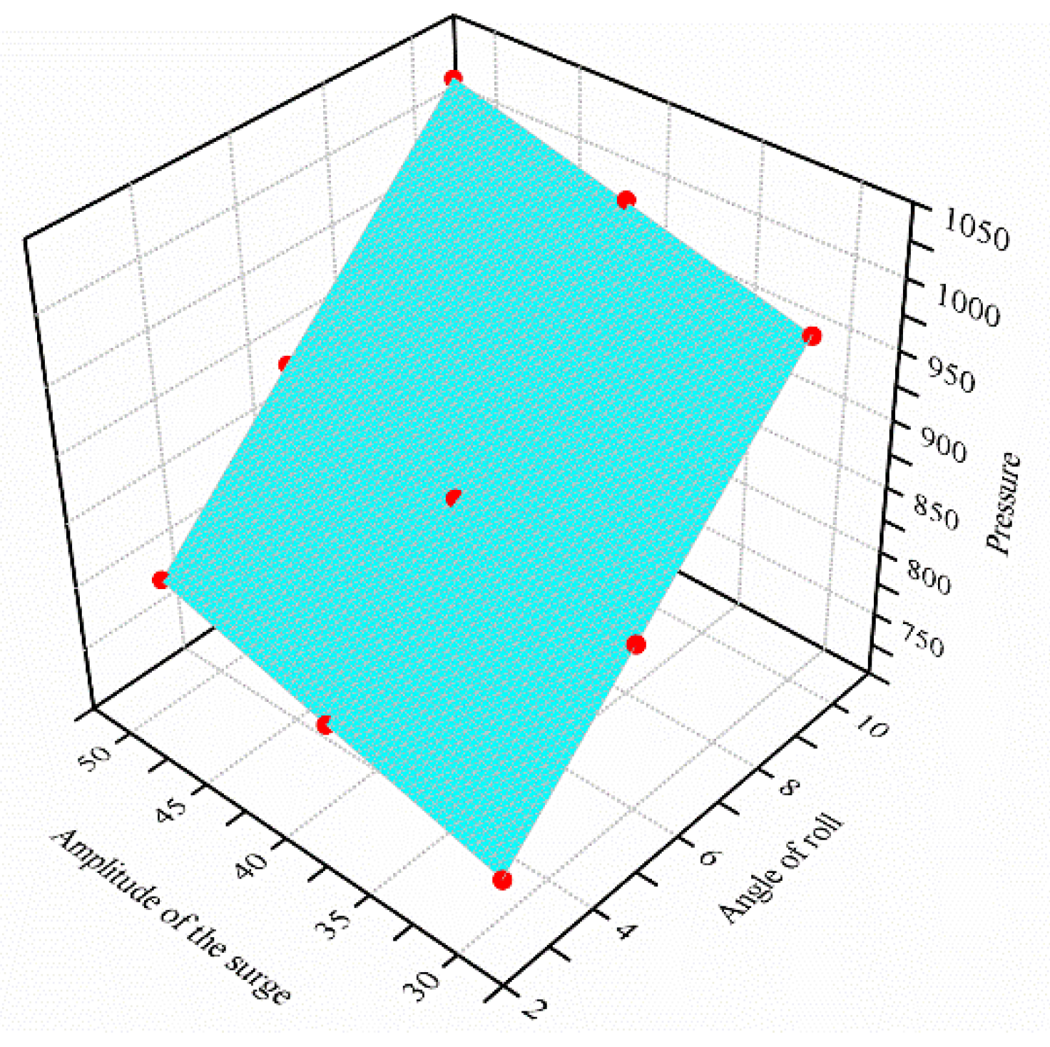
4.4. Effect of Combination Excitation Intensity on Liquid Sloshing

To further explore the influence of combination excitation intensity on sloshing behavior, the variation characteristics of liquid surface height and the pressure time-varying characteristics at different positions under different combination excitation intensity conditions were compared and analyzed, and the influence of combination excitation intensity on peak pressure after sloshing stabilization was explored.

Figure 13 shows the variation curves of the liquid level on lines S1, S3, P1 and P3 with f = 0.58 Hz, λ = 40 mm at roll excitation angles φ of 3°, 6° and 10°. It is shows that with the increase in the amplitude of the roll angle, the peak height of the liquid level increases, and the liquid level at different positions changes periodically, with some differences. In addition, the change in the amplitude of the roll angle has a significant effect on the height change of the liquid level at lines P1 and S3. The reason is that the liquid level mainly sloshes along the diagonal direction of S4 under combination excitation, which makes the height change sharper at the position closer to S4.

Figure 14 shows the variation of the liquid level when the sloshing frequency is 0.58 Hz, the roll angle amplitude is 10°, and the surge amplitudes are 30 and 50 mm. The data in Figure 14 show that the change in the surge amplitude has a more severe impact on the change in the liquid level on the P plane but has a lesser effect on the change in the liquid level on the S plane.

Figure 15 shows the pressure variation at monitoring points P3H50 and S4H50 under different combination excitation conditions. It can be seen that the change in roll angle amplitude has a greater impact on the pressure at the monitoring point, while the surge amplitude has a smaller impact. In addition, The data in Figure 15a,b show that when λ is 50 mm and the roll angle amplitude φ varies in the range of 3~10°, the impact pressure on the S plane increases with the increase in the amplitude of the roll angle, which makes the peak pressure at monitoring point S4H50 show an increasing trend, while the change in the amplitude of the roll angle has little impact on the impact pressure on the P plane. The pressure change at the monitoring point on the P plane mainly reflects the static pressure change caused by the change in the liquid height. Therefore, in the first half of the sloshing cycle, the peak pressure at monitoring point P3H50 increases with increasing amplitude of the rolling angle. In the second half of the sloshing period, the amplitude of the roll angle decreases with increasing roll angle amplitude. The data in Figure 15c,d show that for monitoring point S4H50, the peak pressure is in the first half cycle, during which the impact force of the fluid on the monitoring point is positively correlated with the surge amplitude; thus, the peak pressure of monitoring point S4H50 increases with the increase in the surge amplitude when the roll angle amplitude is certain. For monitoring point P3H50, the peak pressure occurs in the second half cycle, and the pressure at the monitoring point mainly reflects the static pressure change. Therefore, the larger the surge amplitude, the smaller the increase in liquid height. Hence, the surge amplitude increases, and the peak pressure at monitoring point P3H50 decreases.

The above analysis shows that compared with single-degree-of-freedom excitation, the pressures of the monitoring points at different positions under the combination excitation condition are different, and the variation of the peak pressure with the excitation intensity is more complicated. The focus in engineering practice is on the maximum peak pressure generated by sloshing. The data in Figure 12 show that under the combination excitation condition, the monitoring point with the largest pressure peak (of the monitoring points shown in Figure 1) is S4H34. Thus, the following will take the peak pressure of monitoring point S4H34 as the research object to further explore the variation characteristics of the peak pressure at monitoring point S4H34 with changing combination excitation intensity.

As shown in Figure 16, the peak pressure of monitoring point S4H34 varies with the combination excitation intensity (φ and λ). It is shows that when the combination excitation intensity is φ = 3° and λ = 30 mm, the minimum peak pressure at the monitoring point is 731.5 Pa, while when the combination excitation intensity is φ = 10° and λ = 50 mm, the maximum peak pressure at the monitoring point is 1033.37 Pa. The peak pressure values under different combination excitation intensities are basically in the same plane in three-dimensional space. In addition, with the increase in roll angle amplitude and surge amplitude, the impact force of the fluid on the monitoring point will increase, and the peak pressure of monitoring point S4H34 will also increase, showing a linear positive relationship. Among these, the impact of roll angle amplitude on the peak pressure of monitoring point S4H34 is more significant.

5. Conclusions

In this paper, the liquid sloshing characteristics of a tank under a single degree of freedom and combination excitation conditions are studied by numerical simulation combined with experimental verification. The characteristics of the sloshing liquid surface profile and pressure distribution of the liquid tank under typical combination excitation were compared and analyzed in detail. The influence of the combination excitation intensity on the liquid level and the time-varying characteristics of the monitoring point pressure and peak pressure were discussed. The main conclusions are as follows:

(1)

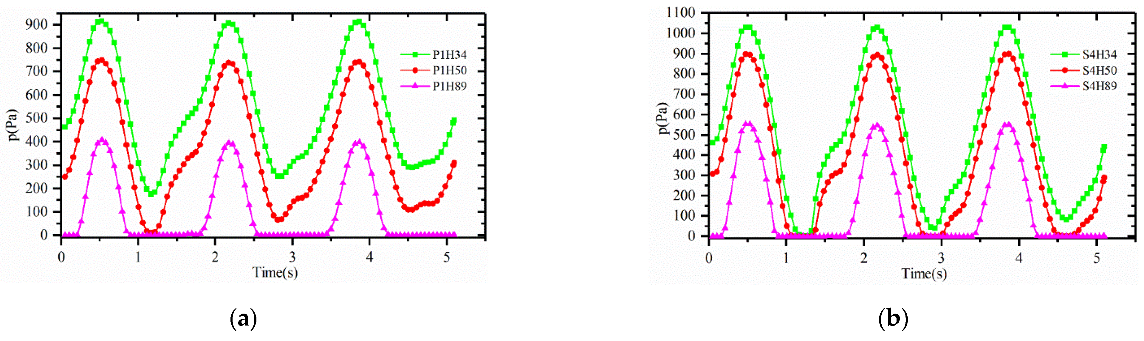
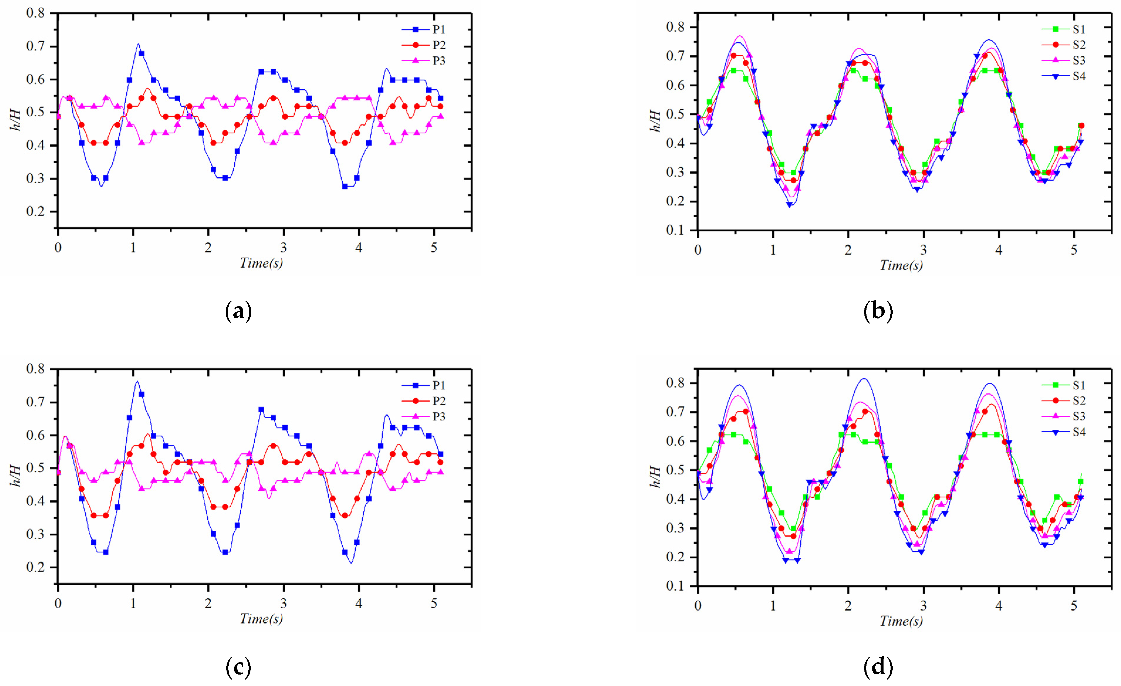
The characteristics of the liquid level variations are obvious under excitation with a single degree of freedom. Meanwhile, the variation in the height of the liquid level noticeably increases with the intensity of single-degree-of-freedom excitation. Moreover, the pressure of the tank wall increases with sloshing. The height of the liquid level and the pressure of the wall have a linear increasing relationship with the sloshing intensity.

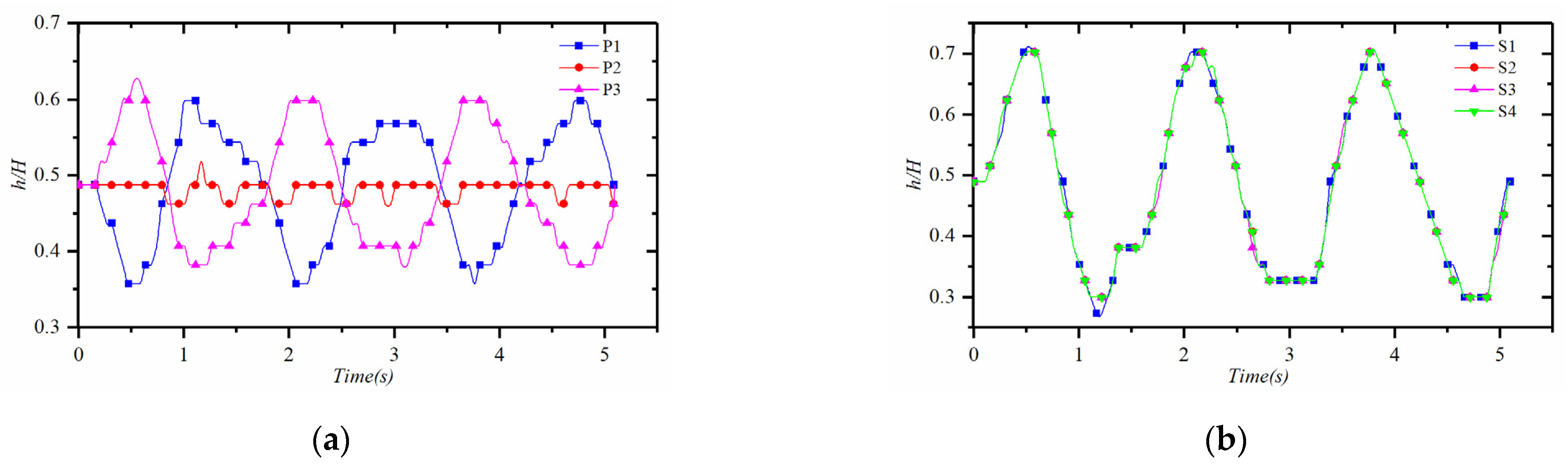
(2)

The height of the liquid level varies periodically under the combination excitation. Furthermore, the liquid level in the cargo tank and the pressure of the wall vary more intensely compared with the single excitation. The peak pressure of the inner liquid, which is greater under the combination excitation, also changes significantly.

(3)

When the liquid tank encounters the combination excitation (roll and surge), the angle of rolling has a great impact on the pressure of the inner wall of the liquid tank. There is a slight increase with the surge amplitude, and the change in the liquid level is also sensitive to the rolling angle, while the surge amplitude is not obvious. Under the combination excitation condition, the peak pressure at the lowest point of the tank diagonal increases linearly with increasing amplitude of the roll angle and the amplitude of the surge.

References

1. Moiseev, N.N. On the theory of nonlinear vibrations of a liquid of finite volume. J. Appl. Math. Mech. 1958, 22, 860–872. [Google Scholar] [CrossRef]
2. Faltinsen, O.M. A nonlinear theory of sloshing in rectangular containers. J. Ship Res. 1974, 18, 224–241. [Google Scholar] [CrossRef]
3. Faltinsen, O.M.; Timokha, A.N. A multimodal method for liquid sloshing in a two-dimensional circular tank. J. Fluid Mech. 2010, 665, 457–479. [Google Scholar] [CrossRef]
4. Budiansky, B. Sloshing of Liquids in Circular Canals and Spherical Tanks. J. Aerosp. Sci. 1958, 27, 58. [Google Scholar] [CrossRef]
5. Kim, D.H.; Kim, E.S.; Shin, S.-C.; Kwon, S.H. Sources of the Measurement Error of the Impact Pressure in Sloshing Experiments. J. Mar. Sci. Eng. 2019, 7, 207. [Google Scholar] [CrossRef]
6. Trimulyono, A.; Hashimoto, H.; Matsuda, A. Experimental Validation of Single- and Two-Phase Smoothed Particle Hydrodynamics on Sloshing in a Prismatic Tank. J. Mar. Sci. Eng. 2019, 7, 247. [Google Scholar] [CrossRef]
7. Yu, L.; Xue, M.-A.; Zheng, J. Experimental study of vertical slat screens effects on reducing shallow water sloshing in a tank under horizontal excitation with a wide frequency range. Ocean Eng. 2019, 173, 131–141. [Google Scholar] [CrossRef]
8. Akyildiz, H.; Uenal, E. Experimental investigation of pressure distribution on a rectangular tank due to the liquid sloshing. Ocean Eng. 2005, 32, 1503–1516. [Google Scholar] [CrossRef]
9. Zou, C.-F.; Wang, D.-Y.; Cai, Z.-H.; Li, Z. The effect of liquid viscosity on sloshing characteristics. J. Mar. Sci. Tech.-Jpn. 2015, 20, 765–775. [Google Scholar] [CrossRef]
10. Doh, D.H.; Jo, H.J.; Shin, B.R.; Min, C.R.; Hwang, Y.S. Analysis of the Sloshing Flows of a LNG Cargo Tank. J. Therm. Sci. 2011, 20, 7. [Google Scholar] [CrossRef]
11. Unal, U.O.; Bilici, G.; Akyildiz, H. Liquid sloshing in a two-dimensional rectangular tank: A numerical investigation with a T-shaped baffle. Ocean Eng. 2019, 187, 106183. [Google Scholar] [CrossRef]
12. Chu, C.-R.; Wu, Y.-R.; Wu, T.-R.; Wang, C.-Y. Slosh-induced hydrodynamic force in a water tank with multiple baffles. Ocean Eng. 2018, 167, 282–292. [Google Scholar] [CrossRef]
13. Zhu, A.; Xue, M.-A.; Yuan, X.; Zhang, F.; Zhang, W. Effect of Double-Side Curved Baffle on Reducing Sloshing in Tanks under Surge and Pitch Excitations. Shock Vib. 2021, 2021, 6647604. [Google Scholar] [CrossRef]
14. Cho, I.H.; Choi, J.-S.; Kim, M.H. Sloshing reduction in a swaying rectangular tank by an horizontal porous baffle. Ocean Eng. 2017, 138, 23–34. [Google Scholar] [CrossRef]
15. Tao, K.; Zhou, X.; Ren, H. A Local Semi-Fixed Ghost Particles Boundary Method for WCSPH. J. Mar. Sci. Eng. 2021, 9, 416. [Google Scholar] [CrossRef]
16. Liu, D.; Lin, P. A numerical study of three-dimensional liquid sloshing in tanks. J. Comput. Phys. 2008, 227, 3921–3939. [Google Scholar] [CrossRef]
17. Tang, Y.-y.; Liu, Y.-d.; Chen, C.; Chen, Z.; He, Y.-p.; Zheng, M.-m. Numerical study of liquid sloshing in 3D LNG tanks with unequal baffle height allocation schemes. Ocean Eng. 2021, 234, 109181. [Google Scholar] [CrossRef]
18. Borg, M.G.; DeMarco Muscat-Fenech, C.; Tezdogan, T.; Sant, T.; Mizzi, S.; Demirel, Y.K. A Numerical Analysis of Dynamic Slosh Dampening Utilising Perforated Partitions in Partially-Filled Rectangular Tanks. J. Mar. Sci. Eng. 2022, 10, 254. [Google Scholar] [CrossRef]
19. Hoch, R.; Wurm, F.H. Numerical and experimental investigation of sloshing under large amplitude roll excitation. J. Hydrodyn. 2021, 33, 787–803. [Google Scholar] [CrossRef]
20. Xue, M.-A.; Jiang, Z.; Lin, P.; Zheng, J.; Yuan, X.; Qian, L. Sloshing dynamics in cylindrical tank with porous layer under harmonic and seismic excitations. Ocean Eng. 2021, 235, 109373. [Google Scholar] [CrossRef]
21. Xin, J.J.; Chen, Z.L.; Shi, F.; Shi, F.L.; Jin, Q. Numerical simulation of nonlinear sloshing in a prismatic tank by a Cartesian grid based three-dimensional multiphase flow model. Ocean Eng. 2020, 213, 107629. [Google Scholar] [CrossRef]
22. Brackbill, J.U.; Kothe, D.B.; Zemach, C. A continuum method for modeling surface tension. J. Comput. Phys. 1992, 100, 335–354. [Google Scholar] [CrossRef]
23. Jung, J.H.; Yoon, H.S.; Lee, C.Y.; Shin, S.C. Effect of the vertical baffle height on the liquid sloshing in a three-dimensional rectangular tank. Ocean. Eng. 2012, 44, 79–89. [Google Scholar] [CrossRef]
Figure 1. Three-dimensional model of cargo tank in experimental test and numerical simulation.
Jmse 10 01100 g001
Figure 2. Six-degrees-of-freedom motion experimental platform.
Jmse 10 01100 g002
Figure 3. Comparison of the liquid-surface profile at different times: (a) roll, (b) surge, (c) front view under combination excitation, (d) side view under combination excitation.
Jmse 10 01100 g003
Figure 4. Liquid level distribution for (a) roll, (b) surge, (c) front view under combination excitation, (d) side view under combination excitation.
Jmse 10 01100 g004aJmse 10 01100 g004b
Figure 5. Variation of the liquid level at different positions: (a) variation of the liquid level on lines P1, P2, and P3 and (b) variation of the liquid level on lines S1, S2, S3, and S4.
Jmse 10 01100 g005
Figure 6. Pressure variation of different monitoring points under roll excitation; (a,b) are the pressures of monitoring points at different heights on lines P3 and S4, respectively; (c,d) are the pressures of monitoring points at 50 mm height on the P and S planes, respectively.
Jmse 10 01100 g006aJmse 10 01100 g006b
Figure 7. Variation of the liquid level under the conditions of surge excitation (f = 0.58 Hz, λ = 50 mm): (a) variation of the liquid level at P1–3; (b) variation of the liquid level at S1–4.
Jmse 10 01100 g007
Figure 8. Pressure variation curves of different monitoring points under surge excitation; (a) and (b) are the pressure distribution curves of monitoring points on P2 and S3, respectively; (c,d) are the pressure of monitoring points at a height of 50 mm on the P and S planes, respectively.
Jmse 10 01100 g008
Figure 9. Surface profile under combination excitation: (a) free surface change diagram and (b) different surface profiles.
Jmse 10 01100 g009
Figure 10. Changes in the liquid level at different times with combination excitation (f = 0.58 Hz, φ = 10°, λ = 50 mm): (a) T/T0 = 0, (b) T/T0 = 0.125, (c) T/T0 = 0.25, (d) T/T0 = 0.375, (e) T/T0 = 0.5.
Jmse 10 01100 g010
Figure 11. Liquid level variation curve under combination excitation: (a) P1–3 liquid level variation curve and (b) S1–4 liquid level change curve.
Jmse 10 01100 g011
Figure 12. Liquid level variation curves under combination excitation (f = 0.58 Hz, φ = 10°, λ = 50 mm): (a,b) are the pressure distribution curves of monitoring points at different heights on P1 and S4, respectively; (c,d) are the pressure at the monitoring point with a height of 50 mm on the P and S planes, respectively.
Jmse 10 01100 g012aJmse 10 01100 g012b
Figure 13. Liquid level variation curves under different roll angle amplitudes (f = 0.58 Hz, λ = 50 mm): (a) and (b), φ = 3°; (c) and (d), φ = 6°; (e) and (f), φ = 10°.
Jmse 10 01100 g013aJmse 10 01100 g013b
Figure 14. Liquid level variation curves under different surge amplitude conditions (f = 0.58 Hz, φ = 10°), (a,b) λ = 30 mm, (c,d) λ = 50 mm.
Jmse 10 01100 g014
Figure 15. Pressure variations at different angles and amplitudes: (a,b) show the pressure curves of monitoring points P3H50 and S4H50 when the surge amplitude is 50 mm; (c,d) show the pressure variation curves of monitoring points P3H50 and S4H50 when the roll angle amplitude is 10°.
Jmse 10 01100 g015
Figure 16. Maximum pressure fitting surface of S4H34 under combination excitation.
Jmse 10 01100 g016