Article

A New Compression and Storage Method for High-Resolution SSP Data Based-on Dictionary Learning

College of Meteorology and Oceanography, National University of Defense Technology, Changsha 410073, China
*
Author to whom correspondence should be addressed.
J. Mar. Sci. Eng. 2022, 10(8), 1095; https://doi.org/10.3390/jmse10081095
Submission received: 30 June 2022 / Revised: 1 August 2022 / Accepted: 4 August 2022 / Published: 10 August 2022
(This article belongs to the Special Issue Technological Oceanography)

Abstract

:
The sound speed profile data of seawater provide an important basis for carrying out underwater acoustic modeling and analysis, sonar performance evaluation, and underwater acoustic assistant decision-making. The data volume of the high-resolution sound speed profile is vast, and the demand for data storage space is high, which severely limits the analysis and application of the high-resolution sound speed profile data in the field of marine acoustics. This paper uses the dictionary learning method to achieve sparse coding of the high-resolution sound speed profile and uses a compressed sparse row method to compress and store the sparse characteristics of the data matrix. The influence of related parameters on the compression rate and recovery data error is analyzed and discussed, as are different scenarios and the difference in compression processing methods. Through comparative experiments, the average error of the sound speed profile data compressed is less than 0.5 m/s, the maximum error is less than 3 m/s, and the data volume is about 10% to 15% of the original data volume. This method significantly reduces the storage capacity of high-resolution sound speed profile data and ensures the accuracy of the data, providing technical support for efficient and convenient access to high-resolution sound speed profiles.

1. Introduction

The ocean has been an important strategic resource for a long time, and countries worldwide are paying increasing attention to research on the marine environment. In the field of marine acoustic application technology, the sound speed in seawater is an environmental parameter that has an important impact on sound propagation in the ocean. Research on the mechanism of the underwater sound field, the detection of underwater acoustic targets, and the calculation and evaluation of underwater sound performance all need to be based on sound speed profile (SSP) data. The marine environment is treacherous and variable, and the sound speed in adjacent seas varies greatly. Low-resolution SSP data cannot meet the accuracy requirements of marine acoustic research. High-resolution SSP data can not only improve the accuracy of marine acoustic applications but also provide strong guarantees for the characterization of the marine environment.
The volume of high-resolution SSP data is large, and the data size at a single data sampling time is on the order of GB. The global sea area is vast and deep, so storing the SSP data of the whole sea places high requirements on the data storage space, which constrains large-scale ocean acoustic research based on the SSP information of the global sea area and is not conducive to using high-resolution SSP data. Therefore, while compressing the storage space required for data and ensuring the accuracy of data recovery, it is necessary to find a reliable and efficient high-resolution SSP data storage method so that the mass data can better meet the needs on standard laptop or desktop computers.
In recent years, dictionary learning [1] has been widely used in the field of sound velocity profile data processing as a feature extraction method. In 2018, Michael Bianco [2] used dictionary learning to extract features and reconstruct ocean SSP data to model ocean SSPs. Then, Kuo et al. [3] proposed range-dependent dictionary learning to retrieve SSPs in order to achieve classification and reconstruction; Sijia et al. [4] compared the modeling capabilities of EOF and dictionary learning to verify that dictionary learning has higher-precision reconstruction capabilities; Qianqian [5] used dictionary learning to invert the sound field of the SSP, reducing the error of the sound field inversion. Existing studies mainly focus on using dictionary learning to invert and reconstruct SSP data, but there is a lack of research and discussion on exploiting the sparse processing and compression capabilities of dictionary learning.
This paper proposes a method for compressing and storing high-resolution SSP data using dictionary learning. The sparse processing of the data is optimized through a dictionary composed of a non-orthogonal basis, and the high-resolution SSP is greatly compressed under the premise of ensuring the recovery accuracy. The method not only saves storage space, but also provides the possibility for the wide application of high-resolution SSP data.

2. Theory and Method

2.1. Mathematical Foundation of Dictionary Learning

A mathematical description of dictionary learning is shown as follows [6]: A data matrix Y m × n = y 1 , y 2 , , y n R m × n can be decomposed into matrix D m × k = d 1 , d 2 , , d k R m × k and matrix X k × n = x 1 , x 2 , , x n R k × n . D is a dictionary matrix, consisting of k k < n normalized column vectors (also called atoms); X is a sparse matrix with a sparsity T (the number of non-zero elements in a column vector of the sparse matrix). In order to make the matrix X more sparse, Y can be approximately represented by Y D X , satisfying Y D X F 2 < ϵ [7]. Thus, the goal of dictionary learning is to solve the dictionary D under the limited sparsity T, so that ϵ reaches the minimum value. The dictionary learning processor is written as
min D , X Y DX F 2 , s . t . i , x i 0 T ,
where x i 0 is the number of non-zero elements of a vector x i . T is a preset sparsity. The ultimate goal is to minimise the residual, Y DX F 2 , where the error is described by the F-norm of the residual matrix, where the F-norm of any matrix A m × n is defined as
A F = i = 1 m j = 1 n a i j 2 ,
The constraint condition to be satisfied for optimisation is x i 0 T . Since there are two unknowns in the optimisation problem, namely, the dictionary matrix D and the sparse matrix X , it is necessary to fix one variable, solve the other variable, and then alternately optimise. Thus, dictionary learning is generally divided into two steps: sparse coding and dictionary update.

2.1.1. Sparse Coding

In Equation (1), when the dictionary matrix D is determined, the sparse matrix X is solved. This process is defined as sparse coding [8]. Sparseness is reflected in the fact that each vector x i has only a few non-zero elements. Sparse coding can be solved by algorithms such as matching pursuit(MP) and basis pursuit(BP) [9]. In this paper, sparse coding is realised by the orthogonal matching pursuit (OMP) algorithm.
The OMP [10] algorithm uses the atomic selection method of the MP algorithm, which has a faster convergence rate. In this algorithm, the residual vector always remains orthogonal to the selected dictionary atom, so it is guaranteed that the same atom will not be reused, and the result can converge in a finite time. To achieve the effect of orthogonality, the Schmidt orthogonal method needs to be introduced to calculate the residuals [11].
The residual r of the original vector y i can be calculated as
r = y i A ( A T A ) 1 A T y i ,
where matrix A is made of k different atoms that have been selected from the dictionary matrix D . In summary, the algorithm for OMP is as follows:
  • Set iteration time j = 1 , residual r j 1 = y i , preset sparsity T, dictionary matrix D m × k = d 1 , d 2 , , d k , index sequence vector Idx = 0 , matrix A = Ø and original vector y i .
  • Compute p = D T r j 1 , select the element with the largest absolute value in p , and denote its row number as p o s and add it to Idx .
  • Add d p o s to the new last column of matrix A , and compute the sparse coefficient vector s = ( A T A ) 1 A T y i .
  • Compute the residual r j = y i As . If r j meets the accuracy requirements or k = T , stop and generate x i by using the elements in Idx as the row index to fill in the values in s into the corresponding rows of the vector x i in turn, and filling all the remaining positions with 0. Otherwise, j = j + 1 , and go to step 2.

2.1.2. Dictionary Update

Dictionary update refers to the process of obtaining a better dictionary under the premise of a fixed sparse representation. K-single value decomposition (K-SVD) is a commonly used dictionary update algorithm [7,12]. It mainly uses singular value decomposition (SVD) to sequentially optimize K-th dictionary atoms and coefficients.
Assuming the sparse matrix X is known, update the dictionary column by column. When updating the k-th column of the dictionary, denote x T k as the k-th row vector of the sparse matrix X . Y DX F 2 can be written as
Y D X F 2 = Y j = 1 K d j x T j F 2 = Y j k d j x T j d k x T k F 2 = E k d k x T k F 2 ,
where
E k = Y j k d j x T j .
Thus, the optimization problem can be described as
min d k , x T k E k d k x T k F 2 .
Equation (6) is a least squares problem. To obtain appropriate x T k and d k , the SVD method [13] is introduced here to solve the problem, as shown in
E k = U ( Σ V T ) .
U is composed of the eigenvectors of matrix AA T . Σ is a singular value matrix, where the diagonals are singular values σ and the rest are 0. Σ 2 is eigenvalues of the matrix A T A and σ takes the positive square root. V is composed of the eigenvectors of matrix A T A . The obtained U is updated into the dictionary matrix D as a new d k , and Σ V T is updated into the sparse matrix X as a new x T k . Update each x T k by using SVD and keep E k shrinking until it meets the error threshold or the iteration number t. Error threshold can be set according to the required accuracy, whose calculation can refer to Equation (10).

2.2. Method and Process of 3D Ocean Sound Speed Data Compression

The ocean SSP is a vertical section formed by the sound speed in the sea changing with depth. Spatially, ocean SSPs are different at different latitude and longitude positions. The SSPs under the same latitude and longitude also vary according to the time interval. At the same time, the denser the latitude and longitude grid points are, the higher the resolution of the SSP data, and the more accurate the data. Therefore, global SSP data generally are large scale and high resolution and involve long-term series. According to these typical characteristics, dictionary learning is naturally introduced to compress high-resolution global SSP data to save storage space [14].
First, we select a part from the SSP data as the training sample and then randomly select a certain amount of data from the sample to form the initial D . The dictionary learning method is used to train and update the D , and obtain a new D n e w that meets the error threshold or reaches the iteration time t which can be freely selected according to the actual compression requirements, and, generally, should be lower than 10. Finally, use D n e w to sparse the original data to obtain X by OMP to realize the compression of the effective data of the original SSP and store the sparse matrix through a compressed sparse row (CSR), which is one of the mainstream compressed storage methods for the sparse matrix. The sparse coding and compression storage process of the general ocean SSP are shown in Figure 1.
The following shows the specific implementation steps from three aspects: data preprocessing, dictionary learning, and CSR storage.

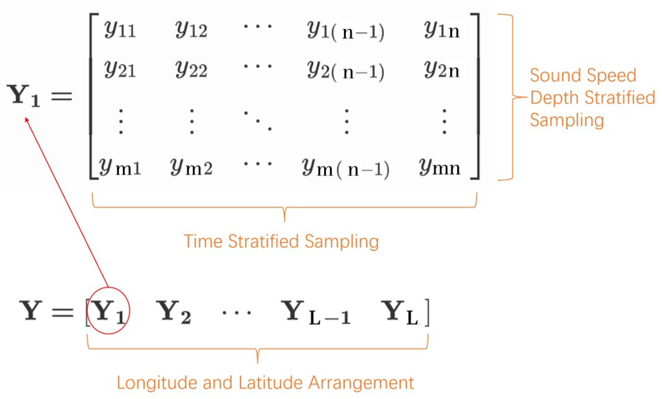
2.2.1. Data Preprocessing

The experimental data come from the “Global High-Resolution Ocean Reanalysis System Development and Product Development” project. The sound speed in the ocean is a function of temperature, salinity, and pressure. Use the empirical formula of the SSP to calculate global high-resolution ocean SSP data, according to the longitude, latitude, ocean temperature, salinity, and water depth data of the global seas [15] provided by the global high-resolution ocean reanalysis products.
First, the annual ocean SSP data of each longitude and latitude point are processed separately. For the annual ocean SSP data of a certain latitude and longitude, we combine the sound speed data corresponding to different depths at a single sampling time point into a column vector and then sort by column using the sampling time as a clue to obtain the annual high resolution corresponding to a single latitude and longitude point SSP matrix. Then, all the obtained latitude and longitude point matrix blocks are sorted by column to obtain the high-resolution SSP matrix of the global ocean area. Denote y i j as the sound speed at the jth time point at the ith layer depth. Data matrix construction is shown in Figure 2.

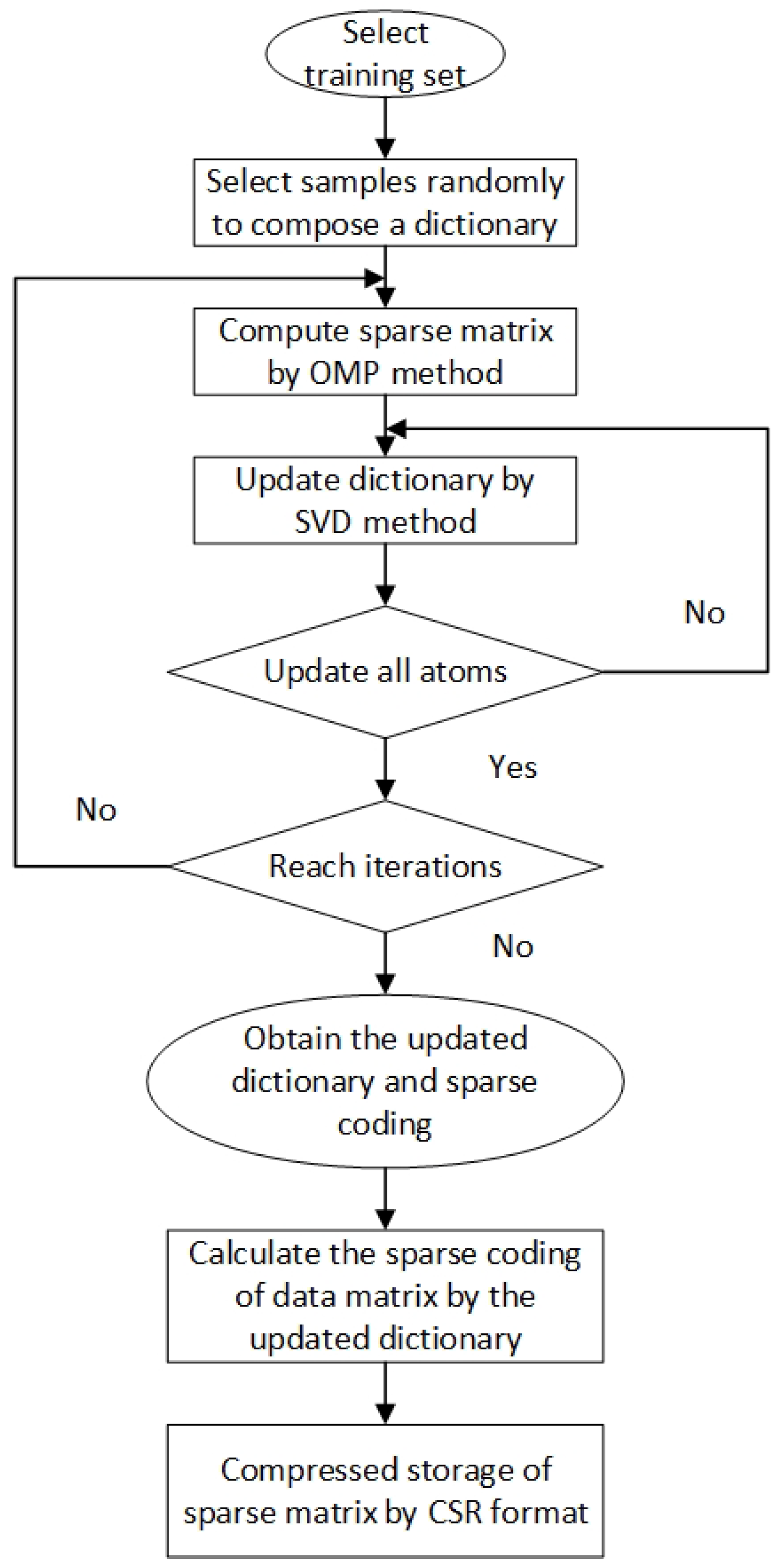
2.2.2. Dictionary Learning
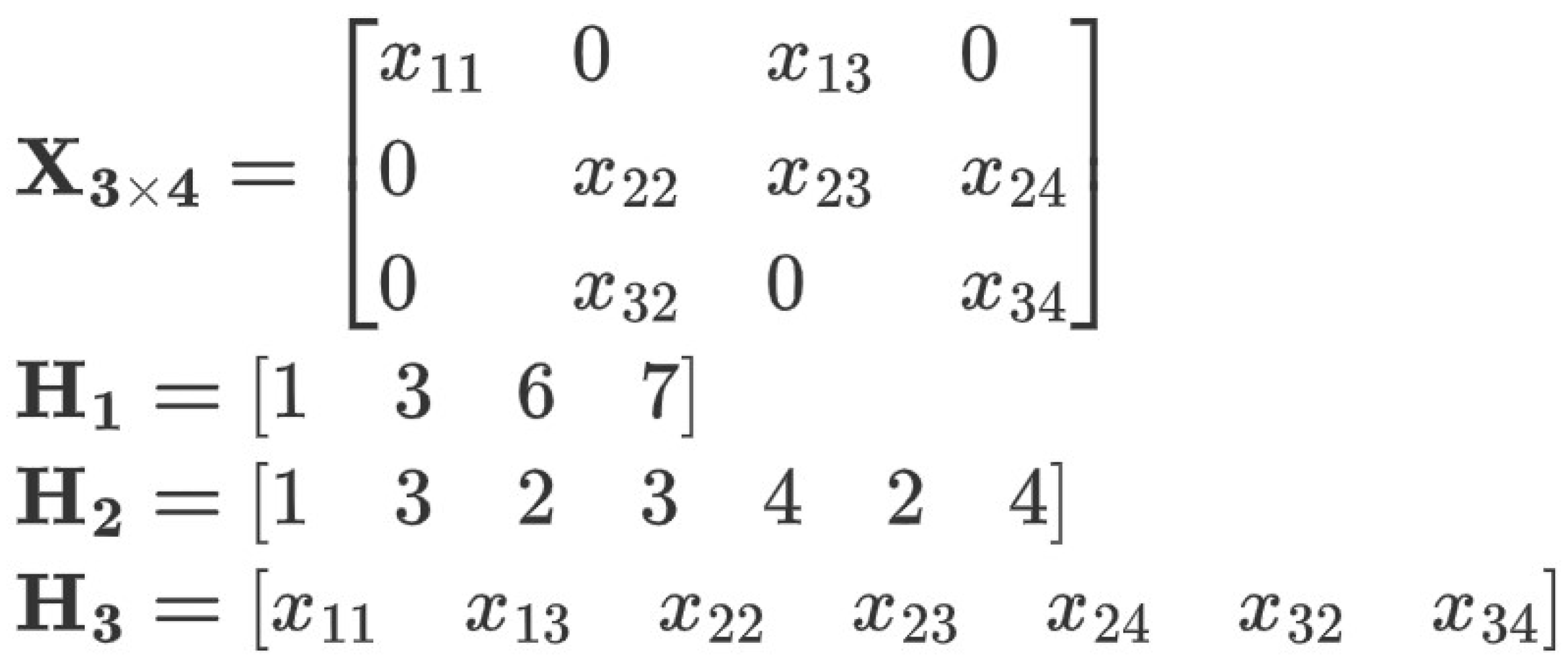
To better train the dictionary, the global sea area high-resolution SSP matrix Y m × n is used as the training sample. We randomly select k samples from it to form the initial dictionary D m × k , where k is generally between 0.02 n and 0.2 n . Based on the initial dictionary and training samples, we set an appropriate sparsity T which can be selected according to the required compression ratio, generally between 2 and 0.1 m . Use the OMP algorithm as described in Section 2.1.1 to sparsely encode the training samples [16].
The K-SVD algorithm as described in Section 2.1.2 is used to update the initial over-complete dictionary column by column, and the residual is calculated. If the residual exceeds the set threshold, OMP algorithm and K-SVD algorithm are repeatedly used to iterate until the error threshold is met or iteration time t is reached. After dictionary learning, the trained dictionary matrix D m × k and the corresponding global high-resolution SSP data sparse matrix X k × n are obtained.

2.2.3. CSR Storage

The CSR storage method is a method for efficiently storing sparse matrices, which is called row format storage. When storing a sparse matrix of order k in the CSR format, assuming that the sparse matrix X k × n has a total of T n non-zero elements, the non-zero elements can be stored in the row vector H 3 in the order of row first. Then, the column numbers corresponding to the non-zero elements of the sparse matrix in the row vector H 2 are stored in sequence, and the position of the first non-zero element in each row in the row vector H 3 in the progressive row vector H 1 is stored. The last bit stores the total number of non-zero elements. Take X k × n as an example in Figure 3, where k = 3, n = 4, T = 2.
The ratio δ C S R of the amount of CSR stored data to the amount of stored data of the original sparse matrix is shown in
δ C S R = n u m ( H 1 ) + n u m ( H 2 ) + n u m ( H 3 ) n u m ( X ) 2 T n + k + 1 k n .
n u m ( · ) is the number of elements in the matrix. The maximum number of n u m ( H 2 ) and n u m ( H 3 ) is T n . The maximum number of n u m ( H 1 ) is k + 1 . The number of n u m ( X ) is k n , which is the number of data in the original sparse matrix. In Figure 3, δ C S R is 2 × 2 × 4 + 3 + 1 3 × 4 = 5 3 . Because T and k are similar, X 3 × 4 is not a sparse matrix and cannot take advantage of the storage advantages of CSR. When 1 T k and 1 < n , δ C S R k + 1 k n < 1 , a better compression storage effect can be achieved for the sparse matrix.

2.3. Performance Evaluation Method

For the compressed storage of high-resolution SSP data, not only the compression capacity but also the error size of the data recovery after compression must be considered to evaluate the reliability of the compression. Therefore, the compression performance is evaluated by the performance evaluation index of the compression ratio δ c o m p and recovery data error.

2.3.1. Compression Ratio

Through dictionary learning, the dense data matrix Y m × n is converted into dictionary matrix D m × k and sparse matrix X k × n , where X k × n is the sparse matrix trained when the sparsity is T, so the maximum number of non-zero elements is T n . The compression ratio δ c o m p can be expressed as the ratio of the sum of the data volume of the three row vectors stored in the compressed dictionary matrix and CSR form to the data volume of the original dense data matrix, as shown in
δ c o m p = n u m ( H 1 ) + n u m ( H 2 ) + n u m ( H 3 ) + n u m ( D ) n u m ( Y ) 2 T n + k + 1 + m k m n .
In the case of a large-scale data matrix, n is much larger than m, T, and k, and Equation (9) can be simplified to
δ c o m p 2 T m .
According to Equation (10), δ c o m p mainly depends on the proportional relationship between T and m. The smaller T m is, the better the compression effect.

2.3.2. Recovered Data Error

The sparsity T is set as the threshold when generating the sparse matrix. Therefore, there is a certain error in the data after compression and storage of the high-resolution SSP data based on dictionary learning. The control error in a reasonable range is also an important criterion for compression performance considerations.
To better compare the size of the error, we choose the average absolute error and the maximum absolute error as the error measurement standard. The average absolute error is abbreviated as M A D , that is, the absolute value of the error of each point is summed and averaged, and the expression is shown in
M A D = 1 m n i = 1 m j = 1 n y i j y i j .
where y i j are the elements in the restored data matrix Y m × n obtained by multiplying the dictionary matrix D m × k and the sparse matrix X k × n . Here, m n is the total number of elements contained in the matrix Y m × n .
The maximum value of absolute error is the absolute value of the maximum error in all data. Since the average value of ocean sound velocity is approximately 1500 m/s, when the absolute error is less than 3 m/s, that is, the relative error is less than 0.2%, the accuracy requirements of most ocean SSPs are met. Therefore, in the process of dictionary learning and compression storage, it is necessary to monitor the average absolute error and the maximum absolute error to ensure that the result meets the set error range.

3. Numerical Results and Analysis

To demonstrate the compression performance of dictionary learning on the high-resolution SSP matrix and to explore the influence of different parameter selections on the δ c o m p and M A D of this method, two locations of 10.95° N, 112.95° E and 0.95° N, 4.95° E were selected to form two different Y 1 . For the high-resolution SSP data of these coordinate points in the whole year of 2014, the sampling time interval is 3 h, so the matrix has a total of n = 8 × 365 = 2920 sampling times and m = 50 . The schematic diagram of the SSP of the two coordinate points is as follows: Figure 4.
The SSP data in Figure 4a vary greatly over time; however, in Figure 4b, the SSP data are relatively stable, with small changes over time. The following analyzes the compression performance of high-resolution SSP data based on dictionary learning in terms of compression rate and recovered data error.

3.1. Influence of Each Parameter in the Algorithm

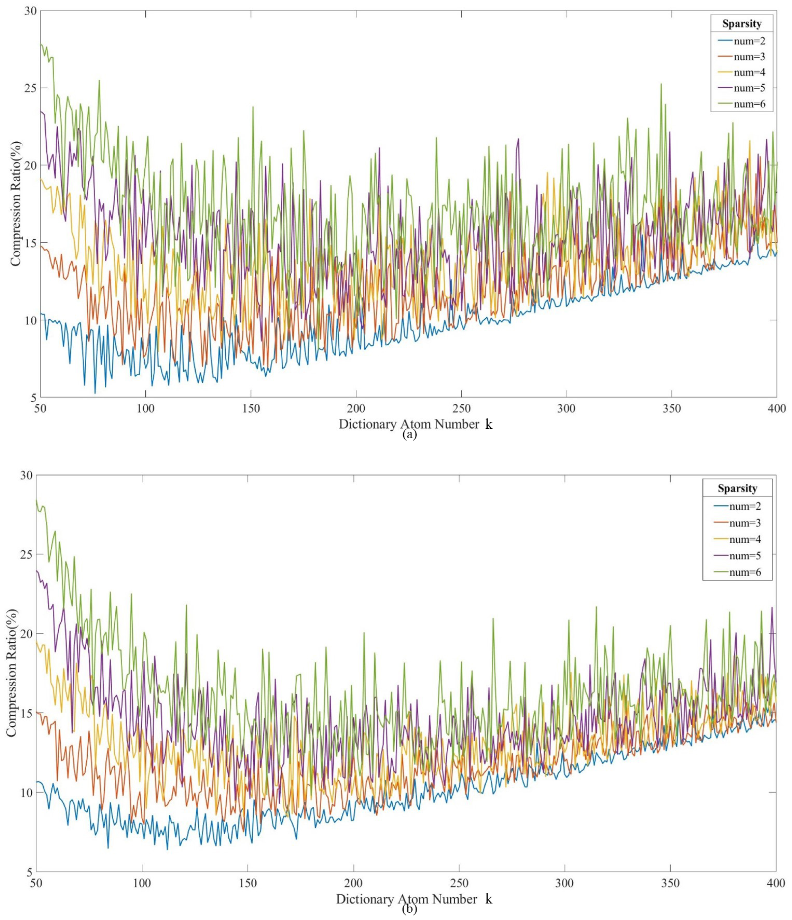
3.1.1. Actual Impact of Parameters on the Compression Ratio

The two locations of SSP data are compressed by dictionary learning, and δ c o m p under different T and different k are calculated using Equation (9). The results are shown in Figure 5.
Figure 5 is the compression result of dictionary learning with two selected samples. The figure shows the influence of dictionary atom number k and the sparsity T on the compression ratio δ c o m p of high-resolution ocean SSP data. In Figure 5, T significantly affects δ c o m p , when k is the same; the smaller T is, the smaller δ c o m p , and the better the compression performance. When T is the same, the minimum of δ c o m p is mainly concentrated in k [ 100 , 150 ] . Since the SSP Figure 5a fluctuates greatly, δ c o m p varies greatly, while, in Figure 5b, the SSP changes gently, so δ c o m p is relatively stable.

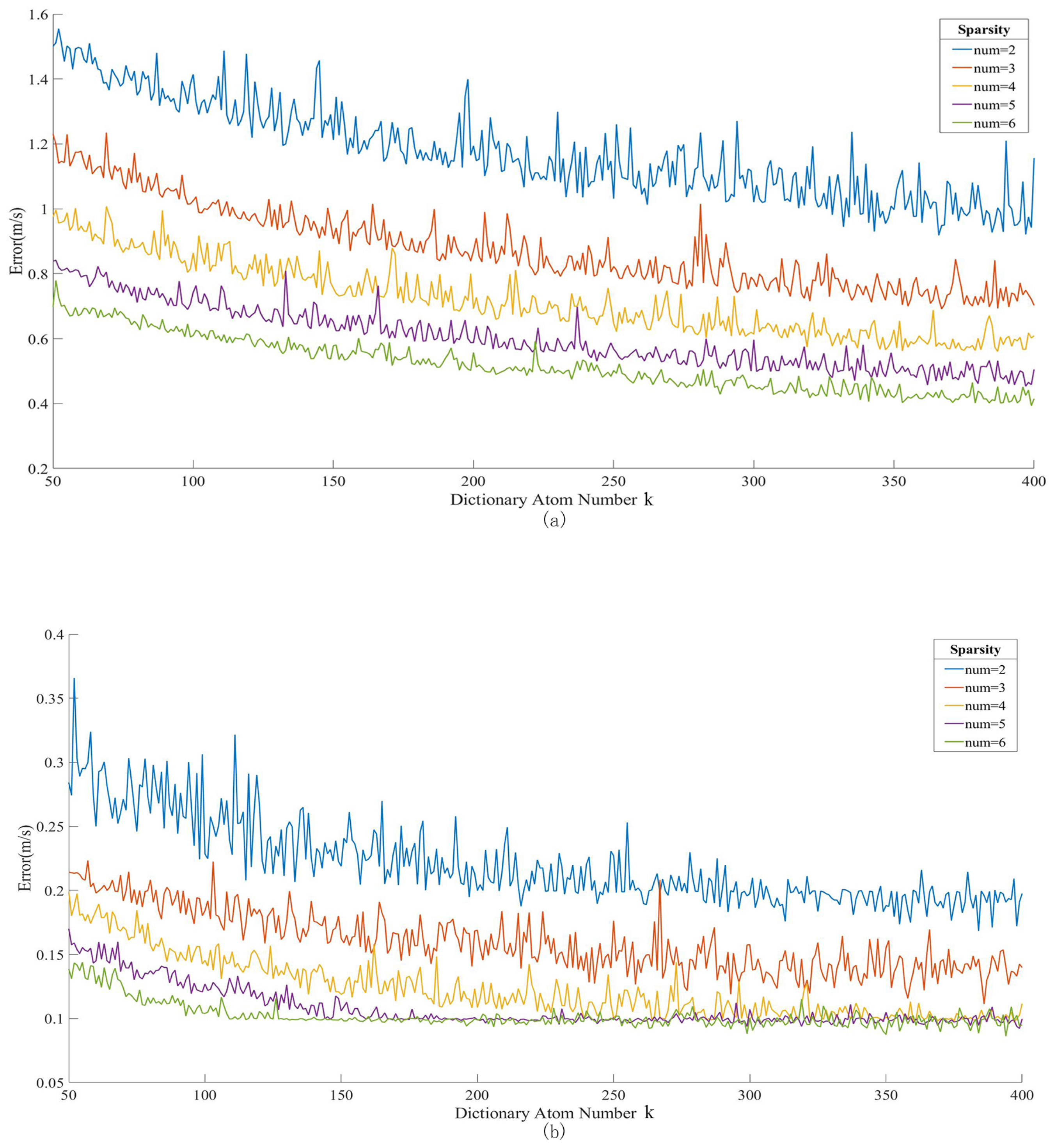
3.1.2. Actual Influence of Parameters on the Error of Recovered Data

Recovery data error tests are performed on the two selected samples, Equation (11) is used to calculate M A D under different T and k, and Figure 6 is obtained.
Figure 5 shows the influence of dictionary atom number k and the sparsity T on the error M A D . The M A D shows a downward trend as k increases when T is the same. When k is the same, the smaller T is, the larger M A D is. Since the SSP of Figure 6a varies greatly, M A D of Figure 6a is larger than that of Figure 6b under the same conditions. When k > 100 , M A D is basically stable.

3.1.3. Selection of Compression Performance Parameters

Through comparative experiments of more samples, the following conclusions can be drawn:
When only focusing on δ c o m p , a small T should be selected, and the selection range of k is in the range of 0.03–0.05n. When M A D is concerned, a larger T should be chosen, and the selection range of k should be larger than 0.03n. Thus, the choice of T depends on the balance between δ c o m p and M A D .
Therefore, before using dictionary learning to compress high-resolution ocean SSP data, it is necessary to analyze the original data scale n and select an appropriate k and T according to application requirements and scenarios to ensure that both compression ratio and recovery accuracy are taken into account.
When the ocean SSP data n are large, due to the limitation of computer calculation performance, k is selected according to the corresponding calculation matrix ability. The larger k is, the more accurate the final recovered data to better ensure that the choice of δ c o m p and T is related to m. When the t is approximately 0.02–0.1n, it is easier to train a good dictionary matrix and ensure the low M A D and high δ c o m p of the data.

3.2. Impact of Data Matrix Organization on Performance

In the actual application process, the depths of various sea areas around the world are different, resulting in different numbers of sample elements of the formed high-resolution SSP matrix and different n of the data matrix, which makes it difficult to directly compress and store dictionary learning. Therefore, this paper proposes two data matrix construction schemes and implementation methods to solve the problem of matrix scale mismatch in the whole sea area. The selected experimental data samples are ocean data of a certain area of the Pacific Ocean (400 km × 400 km) and converted into SSP data using the empirical sound speed formula. The experimental data have a total of 1600 latitude and longitude points, each of which has 2920 time sampling points throughout the year, and the maximum depth is 5906 m.

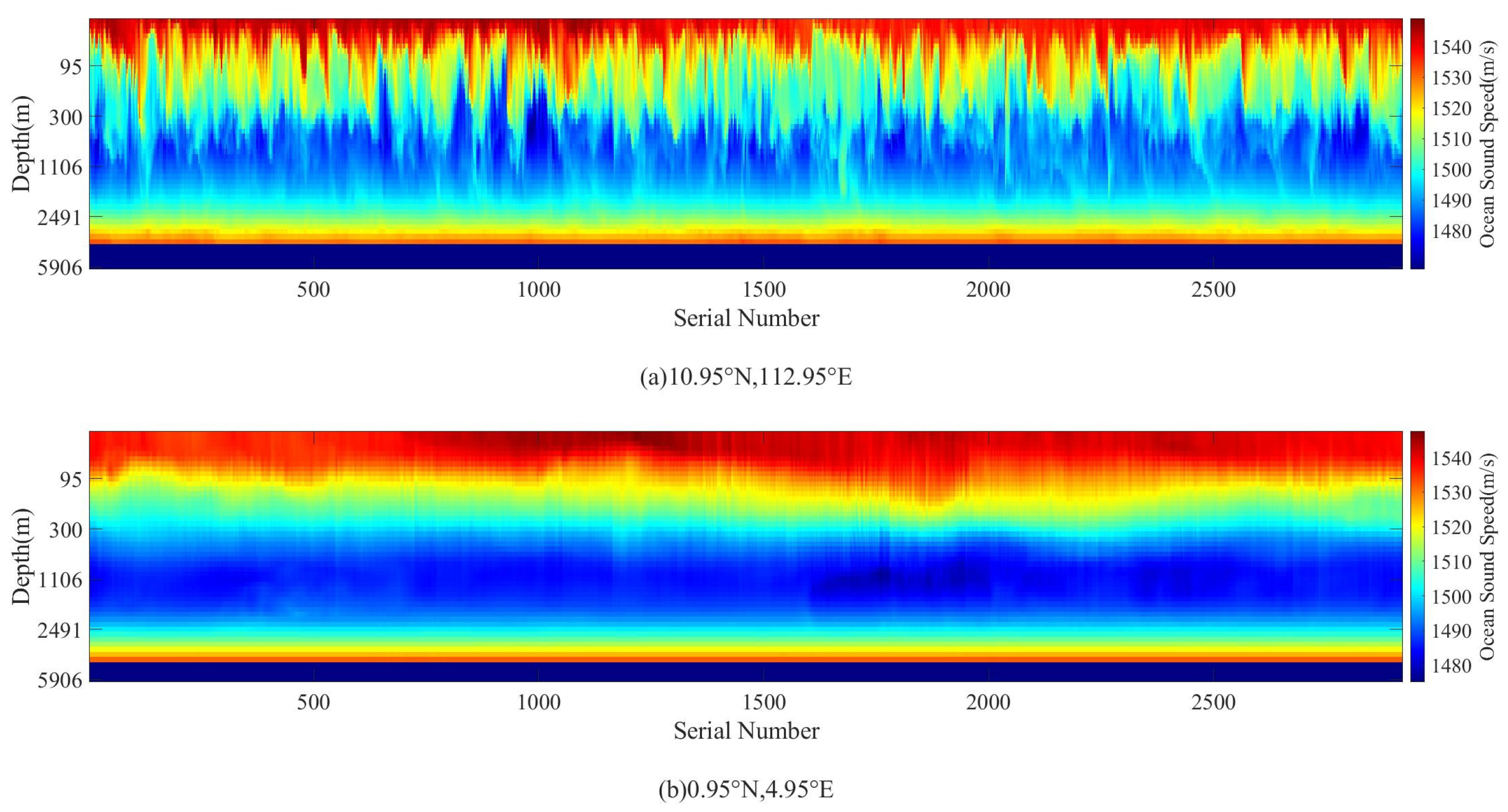
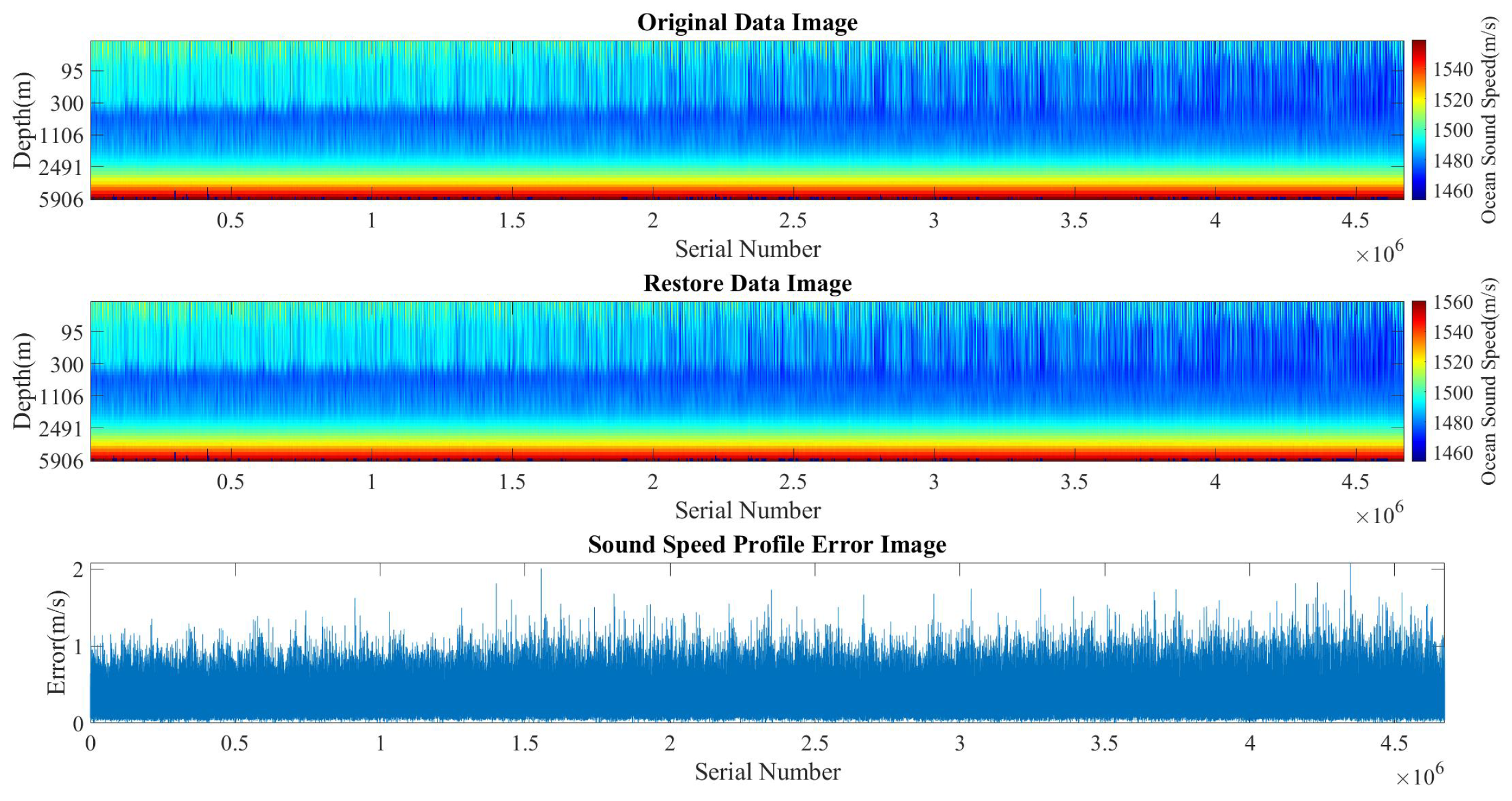
3.2.1. Spatio-Temporal Structure

The spatio-temporal combination structure is a data matrix construction method that arranges spatio-temporal information in an orderly manner to form a super-large-scale matrix. That is, the size of the generated matrix is 50 × 4,672,000. Due to the large number of samples, the method of selecting a training set to train a complete dictionary is used to obtain a dictionary matrix that matches the data matrix. This method is suitable for use on machines with high computing performance and large memory capacity.
A typical SSP is divided into three layers: a mixed layer, a maincline layer, and a deep-water isothermal layer. In the deep-water isothermal layer, the sound speed increases with a positive gradient. The analysis shows that the data of this sea area have reached the respective deep-water isothermal layer. Therefore, they can be interpolated and extended according to their different changing trend to make them unified to 5906 m, which satisfies the largest 50-layer data structure of the matrix, and thus a high-resolution SSP matrix with a scale of 50 × 4,672,000 can be obtained.
We randomly sample this matrix to ensure robustness of the process, select n = 10,000 samples to form the training set, and select k = 2000 to form the initial dictionary for training. According to that described in Section 3.1, we set T = 3 to better obtain compression gains and error data analysis. After the shrinking is complete, we restore the data as described in Section 2.2 for comparison, as shown in Figure 7.
Table 1 shows seven sets of experimental data of dictionary learning compression performance parameters under the spatio-temporal combination structure.
Under n = 10 , 000 , k = 2000 , and T = 3 , δ c o m p of using dictionary learning to compress and store the high-resolution ocean SSP matrix is stable at approximately 12%, M A D is less than 0.5 m/s, the maximum error does not exceed 3 m/s, and the relative error is approximately 0.2%, which meets the accuracy requirements of the SSP data.

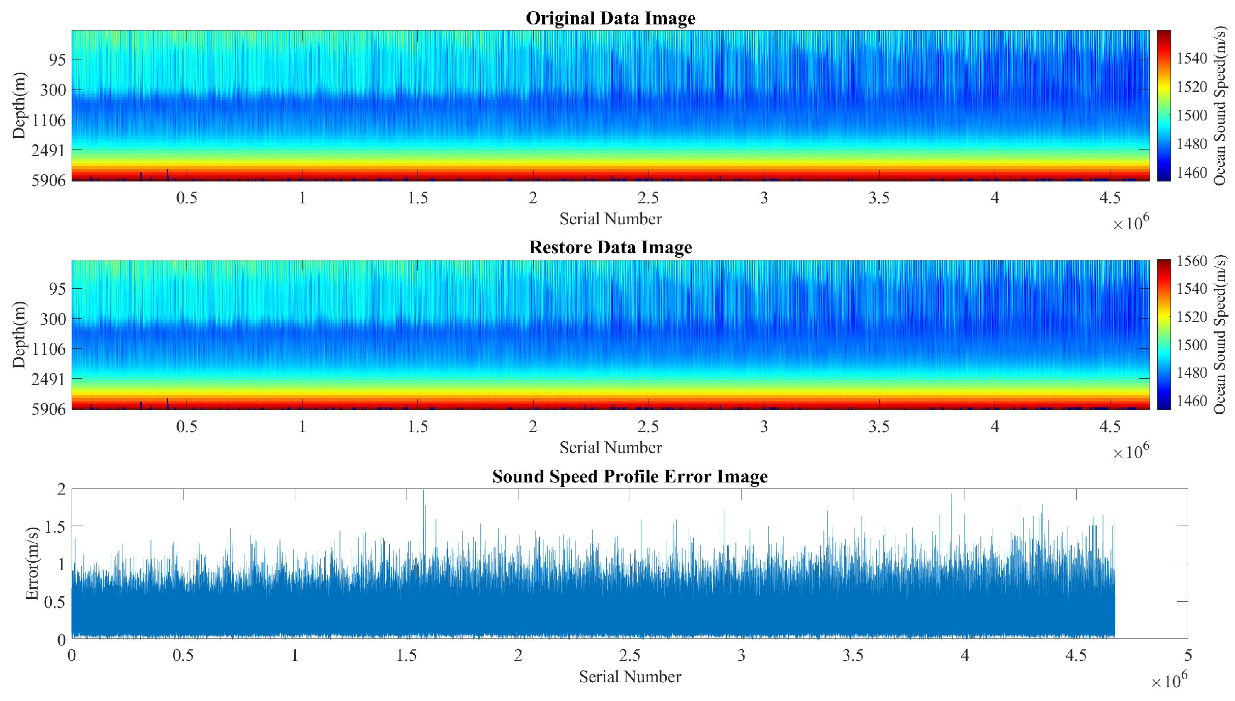
3.2.2. Spatial Discrete Structure

When computing performance and memory is low, the spatial discrete structure can be used. The spatial discrete structure uses dictionary learning to compress all latitude and longitude points, which solves the problem of the inability to establish a unified matrix due to the different depths of each point in SSP data. At the same time, since the change of SSP at the same location is much smaller than change of different locations, separate dictionary learning for each latitude and longitude point can obtain a matrix dictionary that is more in line with the characteristics of the sample and improve the recovery accuracy of large-scale high-resolution ocean SSP data. Due to the small amount of data, it is not necessary to distinguish the training set and the test set to update the dictionary for all samples.
We perform dictionary learning with T = 3 for 1600 latitude and longitude points and select K = 100 . The effect is shown in Figure 8.
Table 2 shows seven sets of experimental data of dictionary learning compression performance parameter under the spatial discrete structure.
Under n = 10,000 , k = 2000 , and T = 3 , δ c o m p of compressed storage is stable at approximately 15%, M A D is less than 0.4 m/s, the maximum error does not exceed 2 m/s, the relative error is approximately 0.13%, and the data recovery accuracy is high. This method has a smaller error than the spatio-temporal structure. However, each point has a corresponding dictionary matrix, the storage data are increased, and δ c o m p is affected to a certain extent.

3.2.3. Performance Comparison

Comparing the two data matrix structures, spatio-temporal structure has the advantages of being large scale and having a high compression rate, while spatial discrete structure has high accuracy, small error, and simple operation.
Spatio-temporal structure, combining the SSP data of all points into a whole, can be trained to obtain a unique dictionary matrix that matches original data. This operation is more concise when recovering data, and the storage resources occupied by the dictionary are greatly reduced; however, because of the matrix, the scale is vast, and substantial memory resources and computing resources are consumed when calculating singular value decomposition. The requirements for computer system configuration are relatively high, and the calculation time is relatively long.
For spatial discrete structure, dictionary learning is performed on the SSP data of each latitude and longitude point, and the corresponding dictionary matrix is generated in turn. Because the size of a single SSP is small, the difference due to compression is not large, and it is easier to generate a dictionary matrix with better performance and reduced error. The error is greatly reduced, the computer configuration requirements are not high, and the calculation time is shorter; however, because the number of dictionary matrices is determined by the number of latitude and longitude points, the relative space of the dictionary matrix occupies more storage space, and the compression rate increases slightly.

4. Conclusions

The data storage and compression of global high-resolution ocean SSPs have high scientific research value and play an important role in exploring ocean acoustic information and developing acoustic applications. The dictionary learning-based high-resolution ocean SSP compression storage method realizes data dimensionality reduction through dictionary learning, transforms a large-scale dense data matrix into a combination of a small-scale matrix and a large-scale sparse matrix, retains the changing trend of the SSP information, ensures a higher compression rate, and achieves precision control, providing a more reliable data compression storage method for high-resolution SSPs.
In dictionary learning, reasonable control of sparsity and dictionary scale can effectively control the compression rate and recovery accuracy of data after dictionary learning. According to different application backgrounds and application requirements, different parameters are selected for data processing, which increases the controllability and flexibility of the method. When the accuracy requirements are not high, for smaller δ c o m p , the spatio-temporal structure can be adopted. On the contrary, when the precision requirements are high, the spatial discrete structure should be chosen.
The compression of high-resolution ocean SSP data through dictionary learning is mainly based on the sparse coding ability of dictionary learning. Some characteristics and laws of the dictionary itself have not been deeply explored. Further in-depth study of dictionaries is required.

Author Contributions

Conceptualization, Y.W. and K.Y.; methodology, Y.W. and K.Y.; software, Y.W. and K.Y.; validation, Y.W. and W.X.; formal analysis, W.X.; investigation, K.Y.; resources, W.X.; data curation, K.Y.; writing—original draft preparation, Y.W. and K.Y.; writing—review and editing, Y.W. and K.Y.; visualization, W.X.; supervision, K.Y.; project administration, Y.W. and K.Y.; funding acquisition, Y.W. All authors have read and agreed to the published version of the manuscript.

Funding

This research was funded by the National Key Research and Development Program of China, Grant No. 2016YFC1401800, and the National Natural Science Foundation of China, Grant Nos. 61379056 and 61972406.

Institutional Review Board Statement

Not applicable.

Informed Consent Statement

Not applicable.

Data Availability Statement

Data available in a publicly accessible repository that does not issue DOIs. Publicly available datasets were analyzed in this study. This data can be found here: http://mds.nmdis.org.cn.

Conflicts of Interest

The authors declare no conflict of interest.

References

  1. Tosic, I.; Frossard, P. Dictionary learning. IEEE Signal Process. Mag. 2011, 28, 27–38. [Google Scholar] [CrossRef]
  2. Bianco, M.; Gerstoft, P. Dictionary learning of sound speed profiles. J. Acoust. Soc. Am. 2017, 141, 1749–1758. [Google Scholar] [CrossRef] [PubMed] [Green Version]
  3. Kuo, Y.; Kiang, J. Estimation of range-dependent sound-speed profile with dictionary learning method. IET Radar Sonar Navig. 2020, 14, 194–199. [Google Scholar] [CrossRef]
  4. Sijia, S.; Hangfang, Z. Sparse Representation of Sound Speed Profiles Based on Dictionary Learning. In Proceedings of the 2020 13th International Congress on Image and Signal Processing, BioMedical Engineering and Informatics, Chengdu, China, 17–19 October 2020. [Google Scholar]
  5. Qianqian, L.; Khan, S.; Fanlin, Y. Compressive acoustic sound speed proile estimation in the Arabian Sea. J. Acoust. Soc. Am. 2020, 43, 603–620. [Google Scholar]
  6. Pali, M.; Rurtz, S.; Schnass, K. Average performance of OMP and thresholding under dictionary mismatch. IEEE Signal Process. Lett. 2022, 29, 1077–1081. [Google Scholar] [CrossRef]
  7. Aharon, M.; Elad, M.; Bruckstein, A. K-SVD: An algorithm for designing overcomplete dictionaries for sparse representation. IEEE Trans. Signal Process. 2006, 54, 4311–4322. [Google Scholar] [CrossRef]
  8. Rubinstein, R.; Bruckstein, A.; Elad, M. Dictionaries for sparse representation modeling. Proc. IEEE 2010, 98, 1045–1057. [Google Scholar] [CrossRef]
  9. Mun, S.; Yazid, H. Performance analysis on dictionary learning and sparse representation algorithms. Multimed. Tools Appl. 2022, 81, 16455–16476. [Google Scholar]
  10. Pati, Y.C.; Rezaiifar, R.; Krishnaprasad, P.S. Orthogonal matching pursuit: Recursive function approximation with applications to wavelet decomposition. In Proceedings of the 27th Asilomar Conference on Signals, Systems and Computers, Pacific Grove, CA, USA, 1–3 November 1993; pp. 40–44. [Google Scholar]
  11. Huang, K.; Aviyente, S. Sparse representation for signal classification. Adv. Neural Inf. Process. Syst. 2007, 19, 609. [Google Scholar]
  12. Zhang, Q.; Li, B. Discriminative K-SVD for dictionary learning in face recognition. In Proceedings of the IEEE Conference on Computer Vision and Pattern Recognition, San Francisco, CA, USA, 13–18 June 2010; pp. 2691–2698. [Google Scholar]
  13. Chen, S.; Donoho, D.; Saunders, M. Atomic decomposition by basis pursuit. SIAM J. Sci. Comput. 1999, 20, 33–61. [Google Scholar] [CrossRef]
  14. Shafiee, S.; Kamangar, F. The Role of Dictionary Learning on Sparse Representation-Based Classification. In Proceedings of the PETRA ’13: Proceedings of the 6th International Conference on PErvasive Technologies Related to Assistive Environments, Rhodes, Greece, 29–31 May 2013. [Google Scholar]
  15. LeBlanc, L.R.; Middleton, F.H. An underwater acoustic sound velocity data model. J. Acoust. Soc. Am. 1980, 67, 2055–2062. [Google Scholar] [CrossRef]
  16. Yang, M.; Zhang, L.; Feng, X.; Zhang, D. Fisher discrimination dictionary learning for sparse representation. In Proceedings of the 2011 International Conference on Computer Vision, Barcelona, Spain, 6–13 November 2011; pp. 543–550. [Google Scholar]
Figure 1. Process of the dictionary learning compression storage.
Jmse 10 01095 g001
Figure 2. Data matrix construction.
Jmse 10 01095 g002
Figure 3. Data matrix construction.
Jmse 10 01095 g003
Figure 4. Schematic diagram of the SSP of the two coordinate points (the total time of 1 year and the sampling interval of 3 h).
Jmse 10 01095 g004
Figure 5. The effect of dictionary atom number k and sparsity T on compression ratio δ c o m p ((a) is 10.95° N, 112.95° E; (b) is 0.95° N, 4.95° E).
Jmse 10 01095 g005
Figure 6. The effect of dictionary atom number k and sparsity T on Error M A D ((a) is 10.95° N, 112.95° E; (b) is 0.95° N, 4.95° E).
Jmse 10 01095 g006
Figure 7. Performance of dictionary learning compression under spatial discrete structure ( k = 100 , T = 3 ).
Jmse 10 01095 g007
Figure 8. Performance of dictionary learning compression under spatial discrete structure ( k = 100 , T = 3 ).
Jmse 10 01095 g008
Table 1. Dictionary learning compression performance parameter under the spatio-temporal combination structure.
Average Error (m/s)Maximum Error (m/s)Compression Rate (%)
0.45782.745513.45
0.48712.345113.22
0.45342.245712.47
0.49652.987411.87
0.46582.912213.45
0.41782.425712.49
0.48442.556711.51
Table 2. Dictionary learning compression performance parameter under the spatial discrete structure.
Average Error (m/s)Maximum Error (m/s)Compression Rate (%)
0.37451.954516.28
0.35441.725315.11
0.35781.987715.87
0.39781.887815.23
0.31471.965214.78
0.37991.853215.26
0.37831.455813.97
Publisher’s Note: MDPI stays neutral with regard to jurisdictional claims in published maps and institutional affiliations.

