Article

The Contribution of the Vendée Globe Race to Improved Ocean Surface Information: A Validation of the Remotely Sensed Salinity in the Sub-Antarctic Zone

1
Department of Physical and Technological Oceanography, Institut de Ciències del Mar, CSIC, 08003 Barcelona, Spain
2
Barcelona Expert Center on Remote Sensing, CSIC-UPC, 08003 Barcelona, Spain
3
Ocean Scope, 29280 Brest, France
*
Author to whom correspondence should be addressed.
J. Mar. Sci. Eng. 2022, 10(8), 1078; https://doi.org/10.3390/jmse10081078
Submission received: 23 June 2022 / Revised: 31 July 2022 / Accepted: 2 August 2022 / Published: 6 August 2022
(This article belongs to the Special Issue Technological Oceanography)

Abstract

:
The Vendée Globe is the world’s most famous solo, non-stop, unassisted sailing race. The Institute of Marine Sciences and the Barcelona Ocean Sailing Foundation installed a MicroCAT on the One Ocean One Planet boat. The skipper, Dídac Costa, completed the round trip in 97 days, from 8 November 2020 to 13 February 2021, providing one measurement of temperature and conductivity every 30 s during navigation. More than half of the ship’s route was in the sub-Antarctic zone, between the tropical and polar fronts, and it passed through areas of oceanographic interest such as Southern Patagonia (affected by glacier melting), the Brazil–Malvinas confluence, the Southern Pacific Ocean, and the entire Southern Indian Ocean. This sailing race gave a rare opportunity to measure in-situ sea surface salinity in a region where satellite salinity measurements are not reliable. Due to the decreased sensitivity of brightness temperature to salinity in cold seas, retrieving sea surface salinity at high latitudes remains a major challenge. This paper describes how the data are processed and uses the data to validate satellite salinity products in the sub-Antarctic zone. The sailing race measurements represent surface information (60 cm depth) not available from drifters or Argo floats. Acquiring measurements using round-the-world sailing races would allow us to analyse the evolution of ocean salinity and the impact of changes in the ice extent around Antarctica.

1. Introduction

Sea Surface Salinity (SSS) is an important factor for understanding the ocean-ice-atmosphere interactions in the Southern Ocean, an area characterized by high winds, strong currents, the presence of fronts and under the influences of ice melting. For instance, the analysis of SSS allows us to monitor changes in sea ice distribution and concentration. The SSS anomalies are linked to sea ice production and water evaporation (positive SSS anomalies) and to melting and precipitation (negative SSS anomalies). Because of the distance and adverse weather conditions, acquiring in-situ salinity measurements in the sub-Antarctic zone is extremely difficult. As a result, satellite observations become a promising option for having continuous and synoptic monitoring of SSS in polar regions.
Since 2009, a new generation of satellites (SMOS from ESA and, later, Aquarius and SMAP from NASA) have provided radiometric measurements in L-band, allowing us to retrieve SSS. In Southern Ocean there are several aspects that hampers the SSS retrieval from L-band measurements. The reduction in sensitivity of brightness temperatures to SSS in cold seas degrades the accuracy of the SSS retrieval in polar regions. Moreover, L-band measurements are seriously affected by land–sea and ice–sea contamination effects. Recently, these difficulties have been addressed over the Arctic Ocean, leading to satellite SSS measurements with enough quality to allow scientific studies [1,2,3,4,5]. However, in the Southern Ocean, SSS has lower variability range than in the Arctic Ocean, and roughness corrections mandatory to retrieve SSS are very challenging due to complex wind–current–wave interactions. Therefore having in-situ data as a ground truth is crucial for validating and enhancing the quality of satellite products in this region. Argo floats are usually used to validate SSS products, however the depth where Argo floats measure salinity is much deeper than the depth where the satellites observe salinity. The difference brings some biases, especially close to the coastal regions where much freshwater is supplied [6,7].
In 2010, the Barcelona World Race (BWR) organizers, scientists from the Institute of Marine Sciences (ICM-CSIC), and members of the Maritime Catalan Forum (FMC) agreed to equip one sailing boat participating in the BWR with a MicroCAT temperature and conductivity sensor, as well as an XCAT transmitter. The objective was to investigate if oceanic races could be used to measure global surface temperature and salinity in real time without interfering with navigation or penalizing the boats’ race performance. Continuous surface monitoring was carried out for the first time during a round trip around the world’s oceans in less than 4 months, contributing to a global study of ocean surface properties and were used to validate remotely sensed salinity products. This was of particular interest because the vessel’s route included rarely sampled regions in the Southern Ocean [8]. After this successful first experience, the collaboration continued, allowing us to collect surface data of conductivity and temperature in the following competitions [9]. In this study we present a new data set, collected in the 2020–2021 Vendée Globe edition.
The Vendée Globe race follows a Clipper route circumnavigation, the fastest circumnavigation of the world. Taking advantage of the strong westerly winds of the Roaring Forties, the route runs from west to east through the Southern Ocean. The Vendée Globe is called after the Vendée département in France, where the event starts and finishes at Les Sables-d’Olonne. From Les Sables d’Olonne, participants onboard IMOCA 60 vessels (a monohull 18 m sailing yacht) navigate the Atlantic Ocean to the Cape of Good Hope; then clockwise around Antarctica, keeping Cape Leeuwin and Cape Horn to port; and finally returning to Les Sables d’Olonne crossing all Atlantic Ocean. The race usually lasts around 24,000 nautical miles (around 44,000 km) and takes place from November to February, aiming to sail through the Southern Ocean during the austral summer. The Vendée Globe is recognized as the greatest endeavour in ocean racing and an extreme challenge of individual endurance. The race presents significant difficulties, such as the strong wind and wave conditions in the Southern Ocean, the competition’s lengthy unassisted duration, and the fact that the route takes racers far from any regular emergency service.
The 2020–2021 Vendée Globe was the ninth edition of the race. It started on 8 November 2020, with the first finishers arriving on 27 January 2021, and last boat arriving on 5 March 2021. There were a total of six female participants among the 33 starters and 25 finishers, which was a record high. The Spanish skipper Dídac Costa completed the race on board of the One Planet Ocean which sailed 24,500 nautical miles in 97 days, 6 h, 27 min and 3 s (Figure 1).
South of 40° S, the Vendée Globe route runs almost parallel to the Antarctic Circumpolar Current (ACC), the world’s largest current, that flows eastward around the Antarctic continent, moving between 100 and 173 Sv [10,11]. The ACC is part of the Meridional Overturning Circulation, which ventilates the Pacific, Atlantic, and Indian Oceans’ deep basins. Between the ACC’s southern edge and the Subtropical Front to the north, three major fronts can be identified: the Southern ACC Front, the Polar Front, and the Sub-Antarctic Front in some places [12,13,14]. The Vendée Globe route crosses the Subtropical front, and the Sub-Antarctic Fronts, where few in-situ data are available.
The first objective of this study is to present a new set of in-situ data (later named as VG2020) obtained thanks to the collaboration between ICM, FNOB and with Vendée Globe organizers. On the other hand, we use this in-situ data to validate the current available remote sensed SSS products from SMOS and SMAP satellites in the sub-Antarctic zone, where few in-situ data are available.

2. Data and Methods

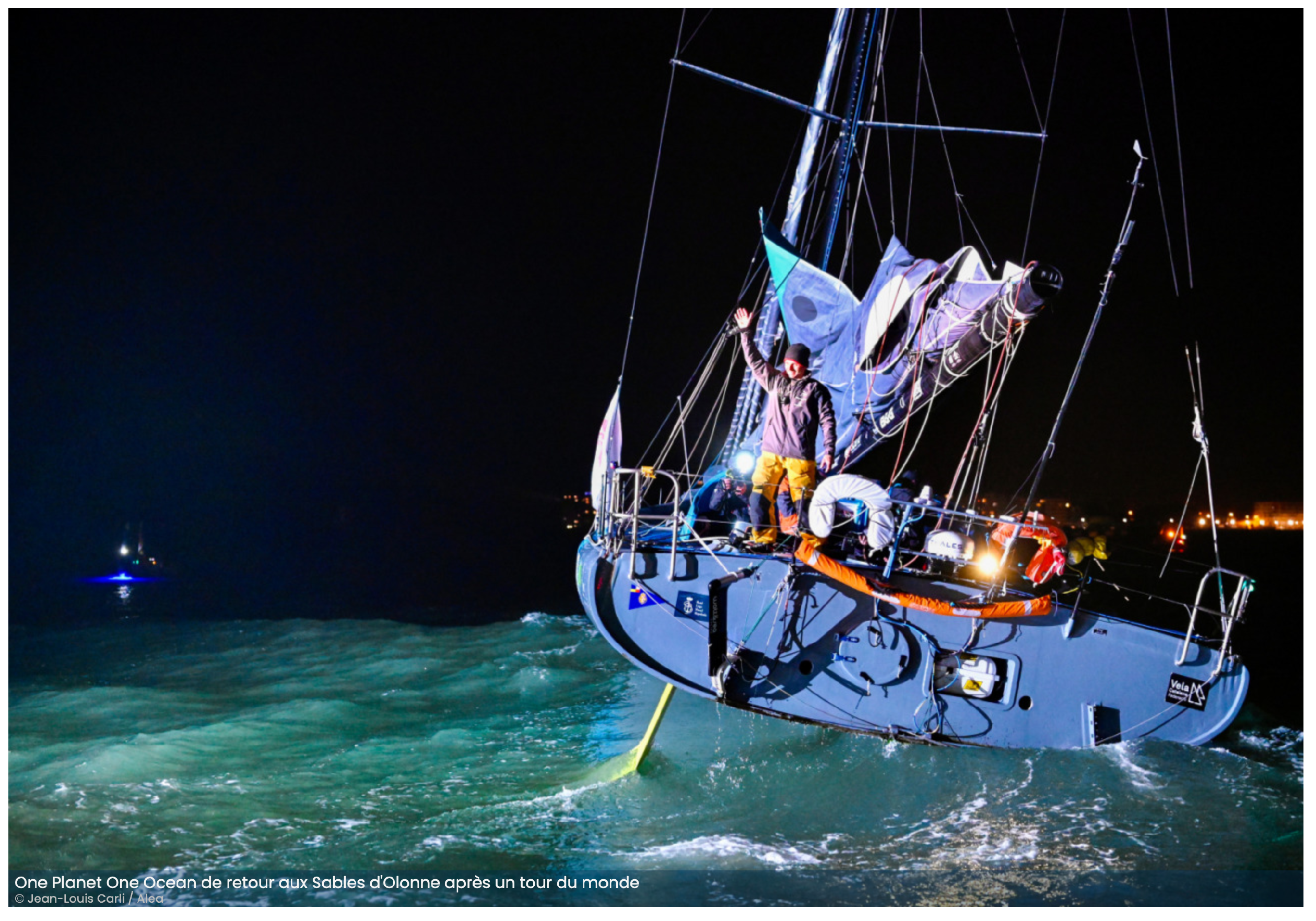
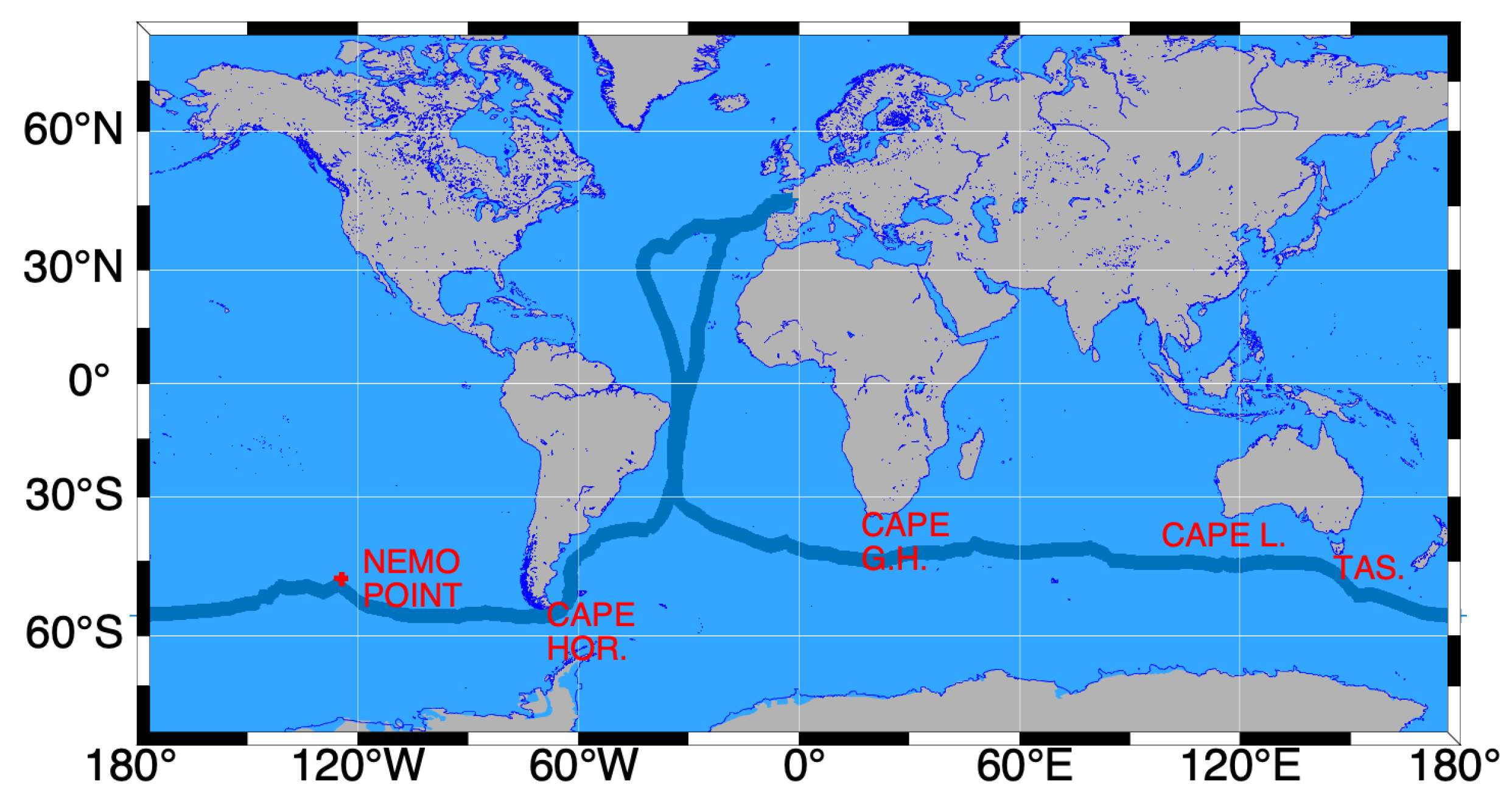
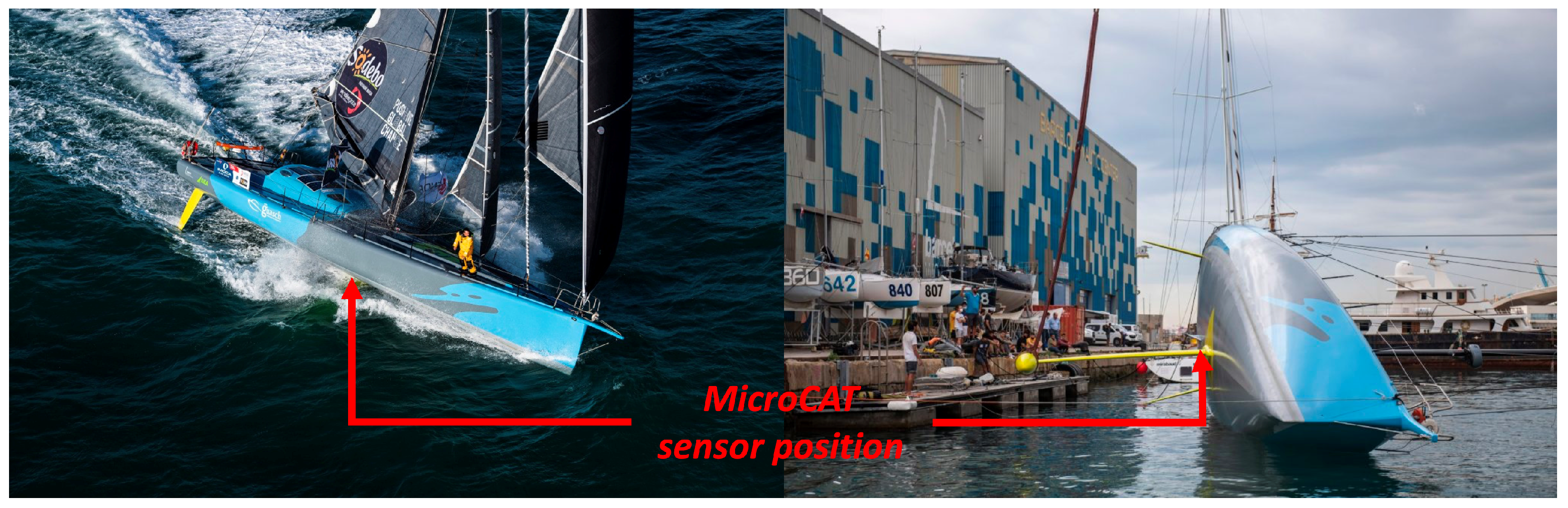
2.1. Vendée Globe In-Situ Data

The Vendée Globe edition 2020–2021 (VG2020) in-situ data have been measured by using a Seabird SBE 37-SI MicroCAT installed in the sailing boat. The SBE 37-SI MicroCAT is a high-accuracy conductivity and temperature sensor equipped with a memory to save the data acquired. Externally powered, the MicroCAT is useful as a stand-alone monitoring device. The conductivity sensor has an accuracy of ±0.0003 S/m (0.003 mS/cm), a resolution of 0.00001 S/m (0.0001 mS/cm) and a stability of 0.0003 S/m (0.003 mS/cm) per month. The temperature sensor has an accuracy of ±0.002 °C (−5 to to 35 °C); ±0.01 °C (35 °C to 45 °C), a resolution of 0.0001 °C and an stability of 0.0002 °C per month. The sensor was calibrated in the factory just before the race started, in September 2020, and installed on the ship in October 2020. The instrument was connected to the ship’s 24 volts batteries through a voltage regulator (7812 with TO220 capsule) so that the input voltage to the sensor remains always constant at 12 volts. This protects the sensor from power overloads. The sensor was installed and configured to autonomously record and store conductivity, temperature and timestamp with a frequency of one measurement every 30 s (two per minute). It has a temperature-compensated crystal oscillator (TCXO, 32,768 Hz) as a real-time-clock frequency source whose accuracy is ±1 min per year (0 °C to 40 °C). In this way timestamp of the data stored can be merged with the ship’s GPS clock to retrieve the position and date of every sample. Once uninstalled after the race, the sensor has been checked in the laboratory to confirm the absence of possible drifts. Therefore no drift corrections were applied to the data.
The positions along the trajectory (Figure 2) where measured using a GPS installed in the boat. The sensor was installed inside the articulated keel which stabilized the boat (Figure 3). It was fixed in this space by means of two flanges anchored in the hull. In this way, the sensor remains nearly at 60 cm bellow the surface, stays in full contact with continuously renewed water. However, the sensor may be impacted by foam if the boat is sailing with the hull too close to the surface, during storm episodes, or when the boat sails too fast. In those cases, data can be affected by as the presence of bubbles that reduce the area of the conductivity sensor, underestimating the conductivity.

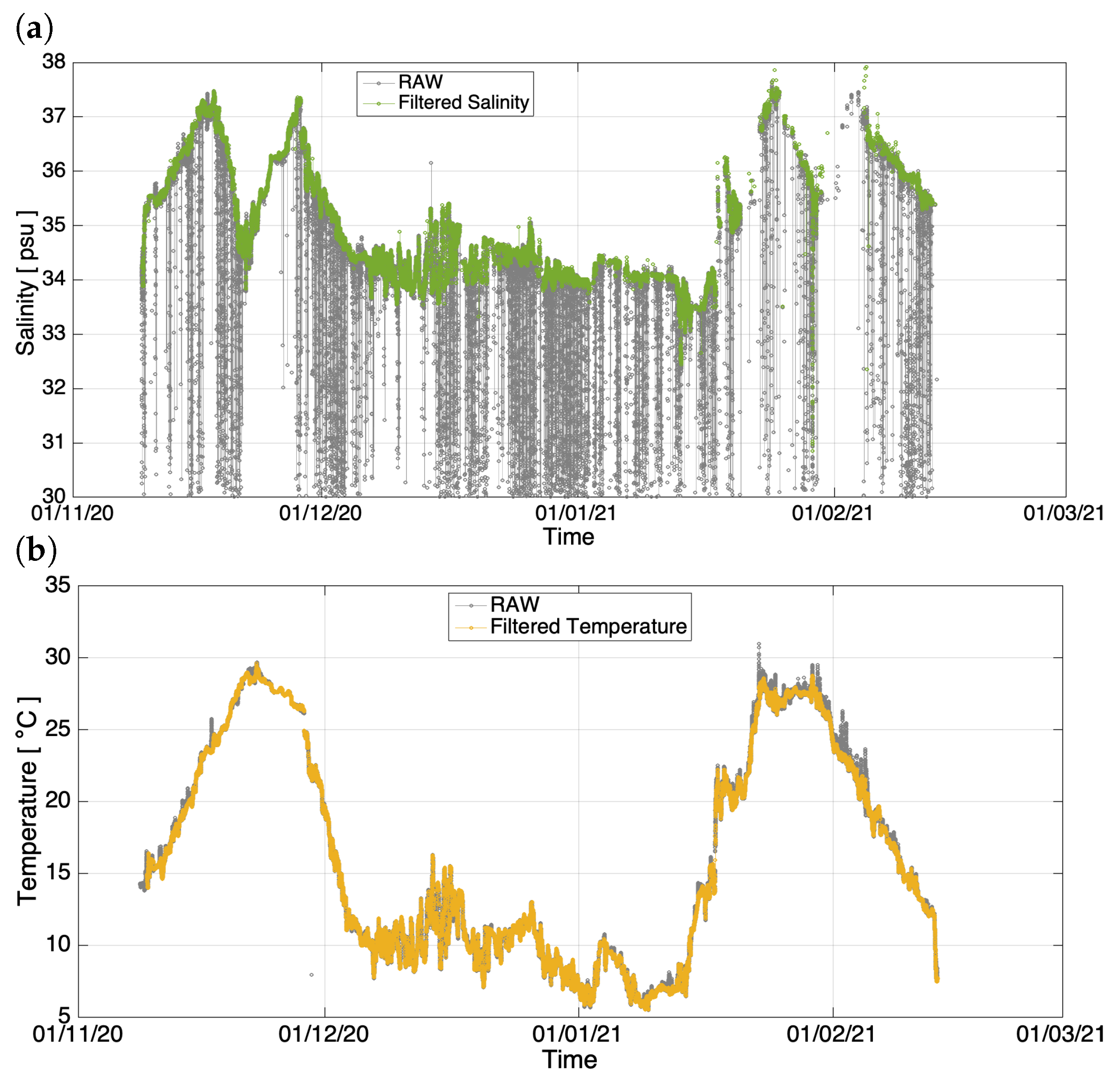
2.2. Vendée Globe Data Filtering Process

The data obtained along the race course need specific assessment as they were measured with a non specialized oceanographic boat. As explained above, the sensor is located in the hull, therefore, the measurements are directly impacted by vessel speed conditions. Temperature (T) and conductivity (C), which are highly linked variables, are the sensor’s primary data.
The filtering process applied to the data is the following:
  • Checking that temperature and salinity are within a geophysical values range. Temperature is filtered out when there are values outside the range of (0–35 °C), and conductivity when the resulting salinity lies outside the range of (30–40 psu). These filtered measurements include records obtained when sensor box was outside the water;
  • The temperature measurement is flagged when (a) there are short spikes denoting that the water might be stagnant, (b) when there are significant differences from the surrounding values and in the absence of strong temperature gradients.
Once the temperature record is considered acceptable, we then flag conductivity when (a) trends are significant opposite to those of temperature and (b) when producing salinity spikes, as detailed bellow. When only conductivity is flagged we considered that the temperature is good and salinity bad. As mentioned above, data are filtered when the local trends of T and C are opposite. In some cases, the water in the box is not renovated, causing an increase (or decrease) in the temperature and conductivity values that are not corresponding to the sea water crossed by the sailboat. If the water container gets stagnant, T rapidly rises (or decreases) and recovers once the water is replaced again. Moreover, under high-hull-speed conditions, the rise of the hull above the water causes air bubbles and foam getting the sensor box, and even empty the sensor box. Bubbles or foam only influence conductivity. These episodes of bubbles and foam entering the sensor box are typically related to the boat’s heading in relation to the wind direction. A lot of foam may come under upwind sailing (i.e., wind blowing 45 to 90 degrees off the heading) especially under rough seas. A downwind sailing may rise the boat over the water, causing the sensor box to dry up. Under crosswind sailing, typically no foam enters the sensor box as boat is attached to the water, and is moving quickly.
A comparison of filtered and original measurements are shown in Figure 4. Abrupt peaks in temperature associated to situations of stagnation of the sensor are removed. Most of the salinity measurements affected by bubbles (abrupt decreases of salinity values) are filtered out. Note that, close to the equator, when the boat was coming back to France at the end of January 2021, the measurements exhibit a decrease in salinity that coincided with an increase in temperature that may reflect the effect of a heavy tropical rain.

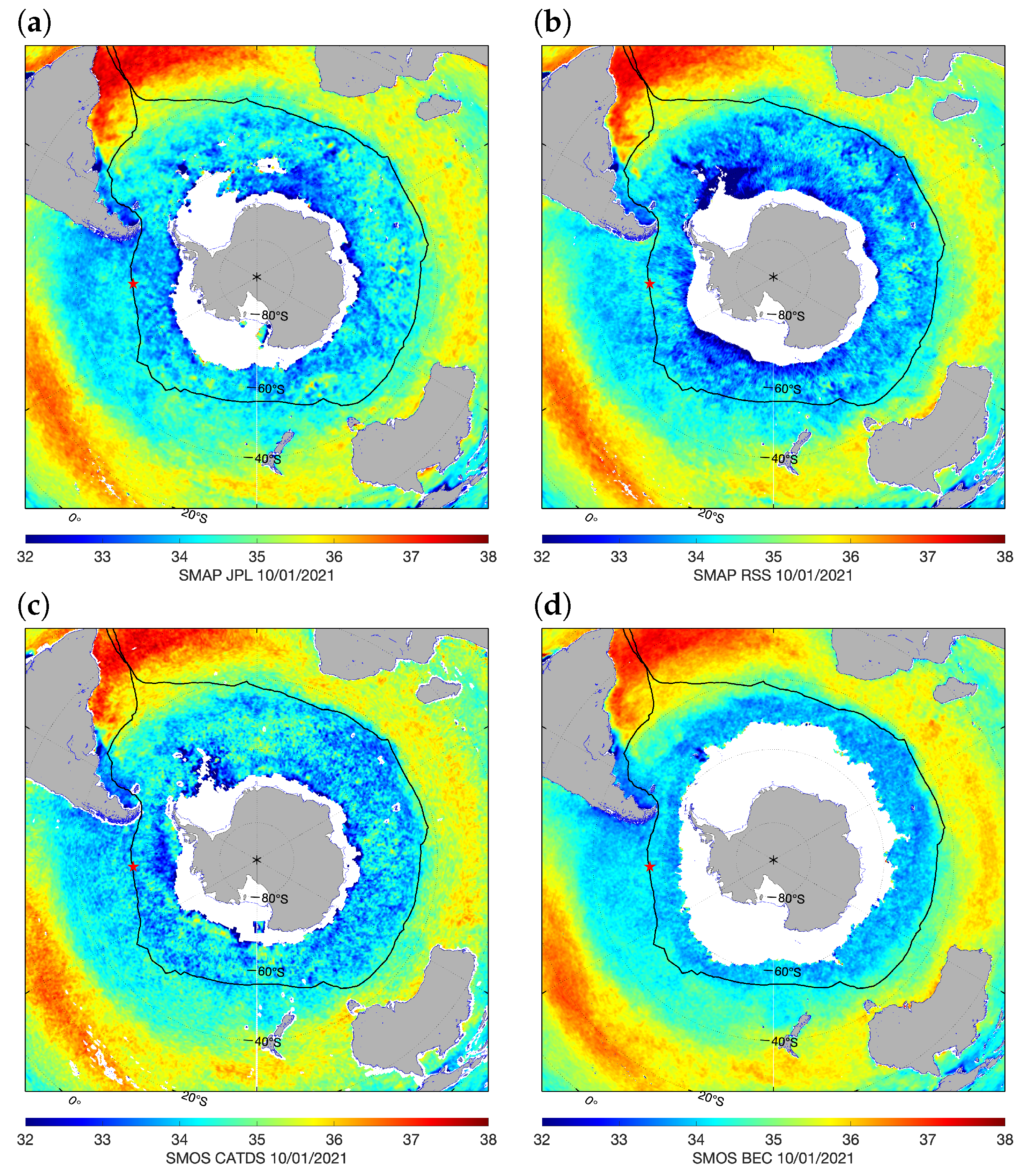
2.3. Remotely Sensed SSS Products

We use four different Level-3 SSS products. Two are derived from the Soil Moisture and Ocean Salinity (SMOS) ESA mission and two from the Soil Moisture Active Passive (SMAP) NASA mission. SMAP JPL v5 and SMAP RSS v4 correspond to 8-day running mean maps on 0.25 degree resolution grids provided by the Jet Propulsion Laboratory [15] and Remote Sensing Systems [16], respectively. SMOS BEC v2 and SMOS CATDS v5 are 9-day running mean product at 0.25 degree and 25 km resolutions respectively obtained from the Barcelona Expert Center on Remote Sensing of the ICM-CSIC [17] and the LOCEAN/IPSL (UMR CNRS/UPMC/IRD/MNHN) laboratory [18]. We have regridded all datasets to a common 0.25° regular grid. Each dataset was accessed on 20 January 2022 from the following links: https://doi.org/10.5067/SMP50-3TPCS, https://doi.org/10.5067/SMP40-3SPCS, http://dx.doi.org/10.20350/digitalCSIC/12601 and https://doi.org/10.17882/52804.

3. Results and Discussion

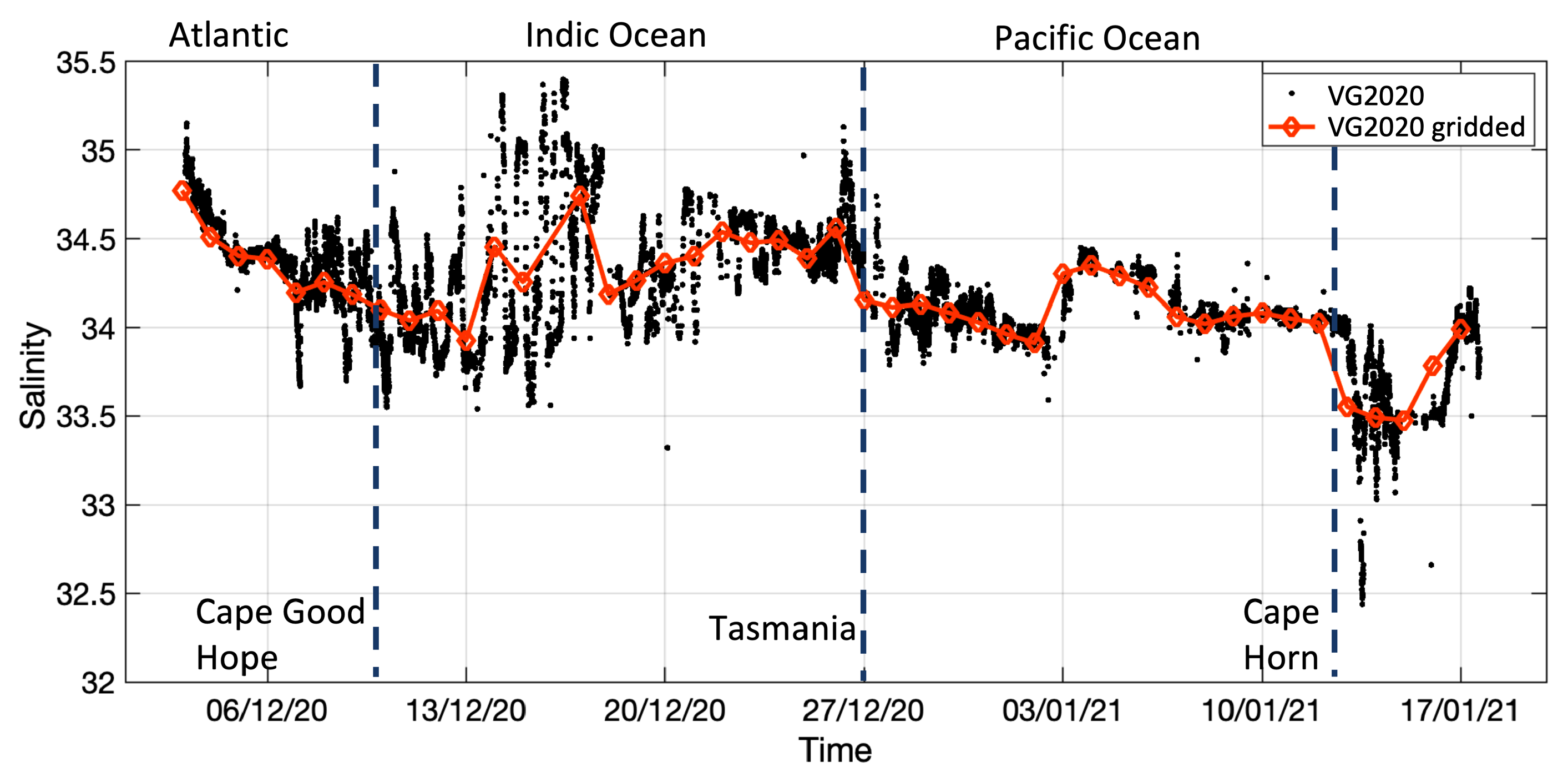
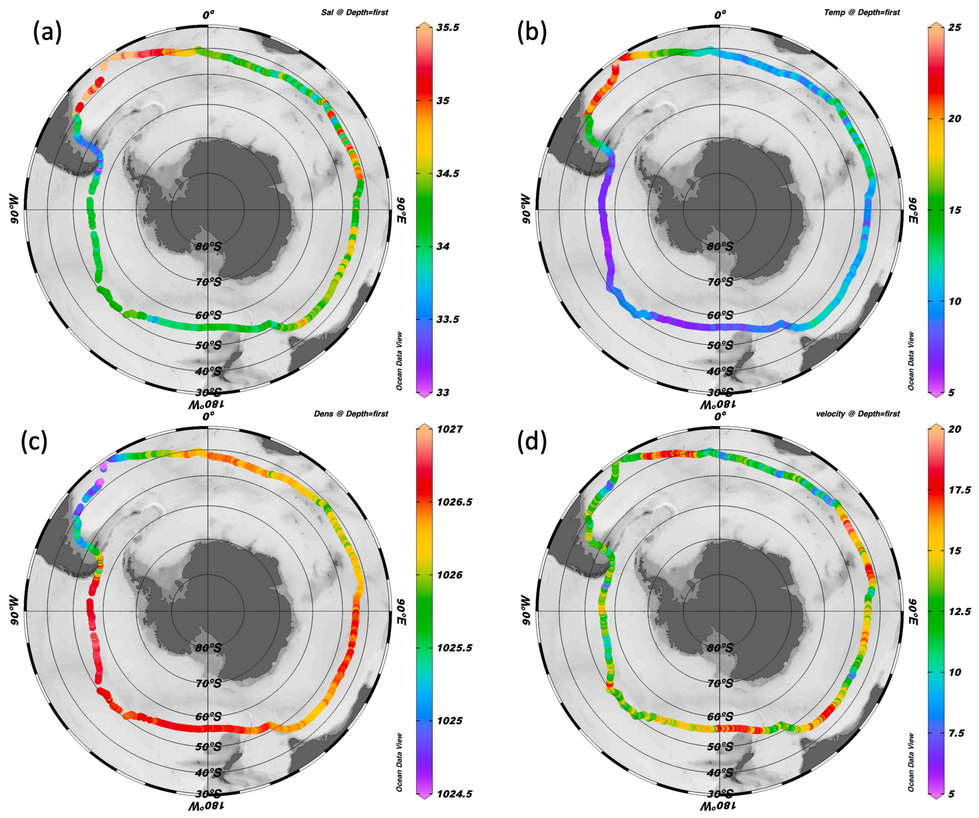
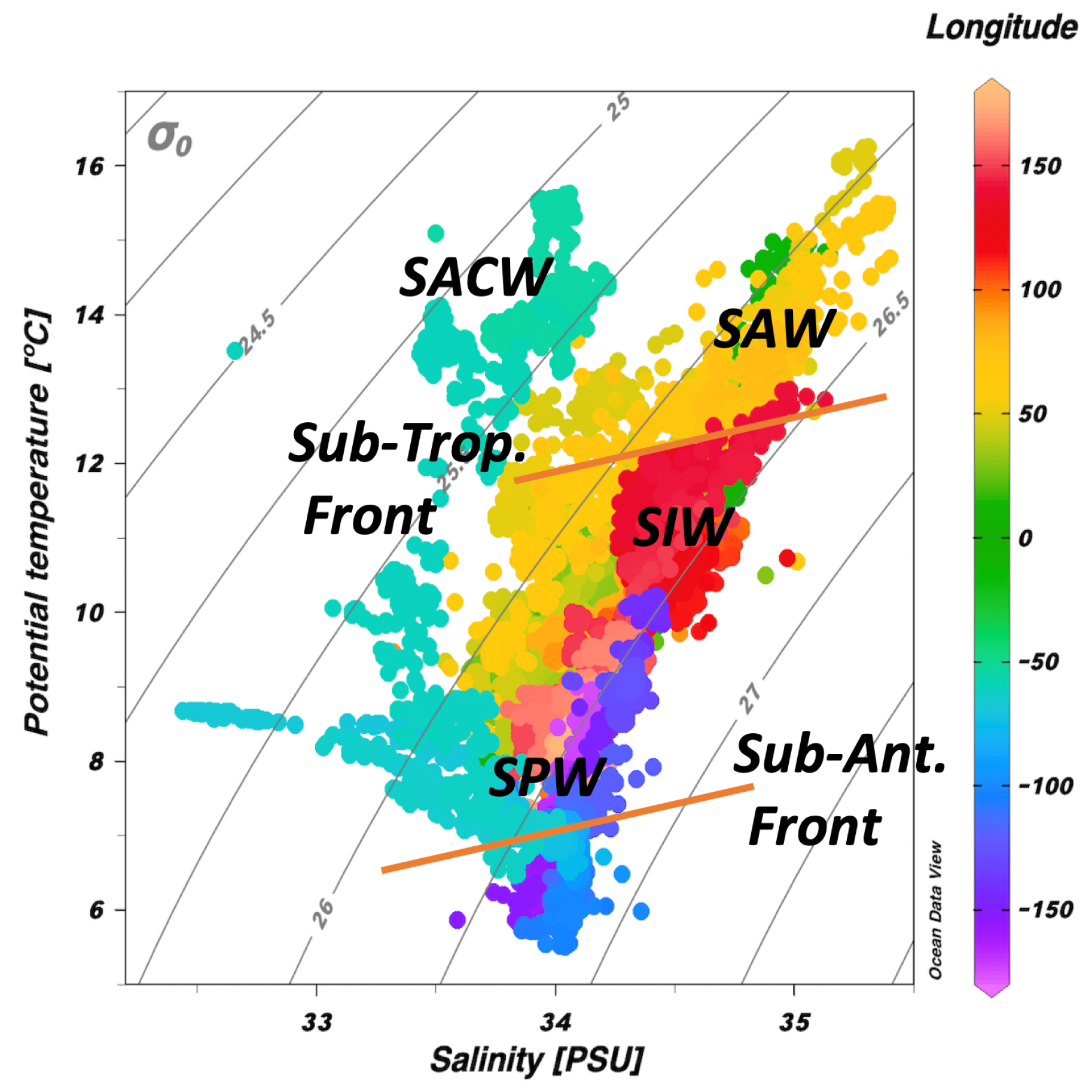
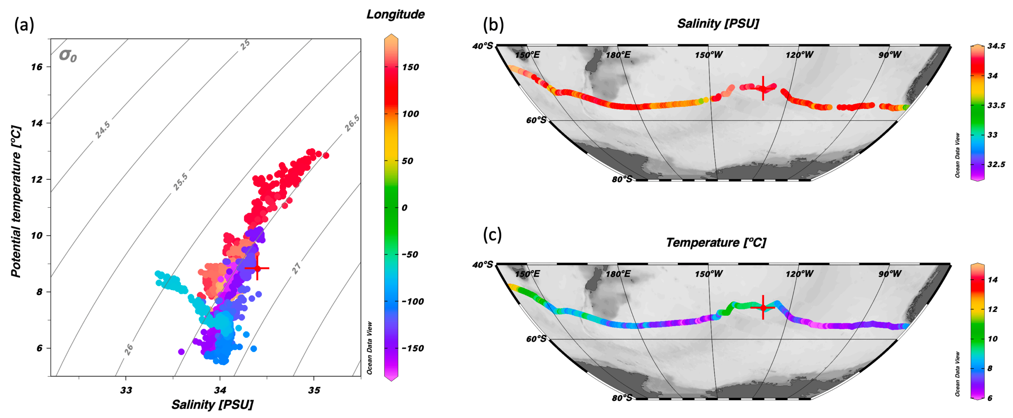
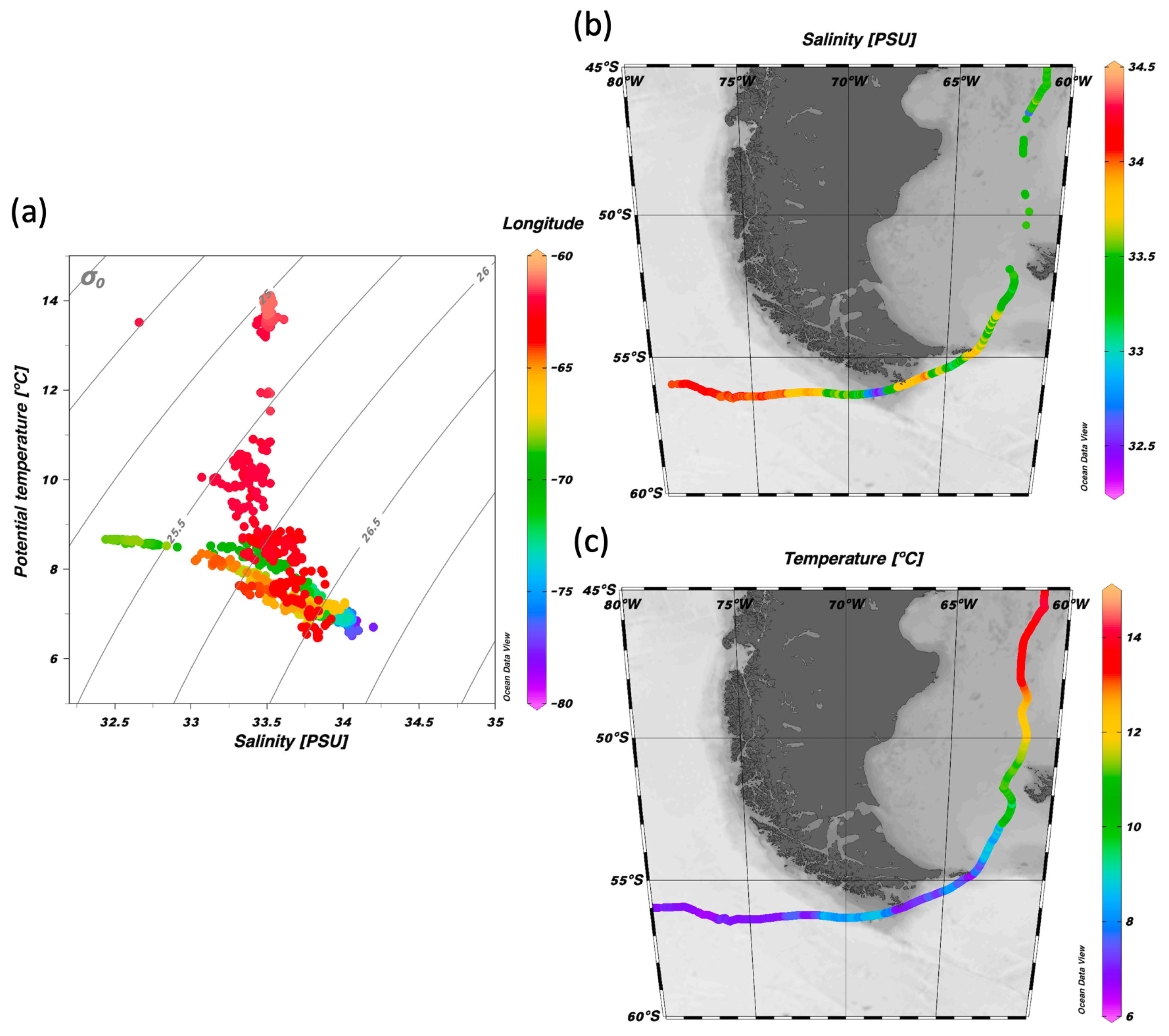
3.1. In-Situ Data Results in the Sub-Antarctic Zone

More than half of the ship’s path was through the sub-Antarctic zone, between the subtropical and polar fronts. The in-situ filtered temperature, salinity, density and velocity of the boat along the trajectory southern than 40° S are shown in Figure 5. When the boat reached 40° S for the first time, heading east, appears to be likely under a stormy weather helping the skipper to navigate downwind to make significant progress. The boat traveled through the Agulhas retroflection zone and then it traversed the whole Southern Indian Ocean. At roughly 0° E, the ship crossed the subtropical front (both temperature and salinity decreased) and then again at around 50° E (increase both in temperature and salinity), and finally in 90° E (temperature and salinity decrease). The subantarctic front was crossed for the first time after Tasmania (a clear temperature and salinity drop), then crossed again at 140° W (increase in temperature and salinity) and at 130° W (temperature and salinity decrease). After traversing the whole Pacific Ocean, the Vendée Globe trajectory reaches the south of Patagonia and Cape Horn, an area susceptible to have relevant freshwater inputs due to ice melt, and again returns north through the Atlantic Ocean to finish the race.
Temperature–Salinity ( θ S) diagram of in-situ data obtained south of 40° S (Figure 6) allow us to differentiate the saltier (>34.5 psu) and hotter (>13 °C) SubAntarctic waters (SAW), the subtropical front, Southern Indian Ocean waters (SIW) (10–15 °C, and 34–35 psu), the sub-antarctic front, and the fresher (33.5–34.5 psu) and colder (5–10 °C) Southern Pacific waters (SPW). Isopycnals refer to the density anomaly ( σ θ ) at 0 m (surface), since all the θ S points lie at surface, computed as σ θ = σ 0 = ρ −1000 (kg/m3).
If we focus only in the Pacific Ocean (Figure 7), we can detect the boat crosses of the Sub-Antarcic front from south to north (longitude 140° W) gaining 2 °C and 0.5 psu and again from north to south at longitude 130° W.
When the vessel arrived to the South Patagonia-Cape Horn, encounters continental-influenced waters (Figure 8), recording a significant drop in salinity of 1.5 psu due to glacier melting. Those waters have low salinity (32–33 psu), low temperature (8–9 °C) and relatively low density (25–25.5 kg/m3). Later as it navigated northwards, waters temperature increased arriving at the Brazil-Malvinas confluence and further north reaching to South Atlantic Central Waters (14–15 °C, 33.5–34 psu).

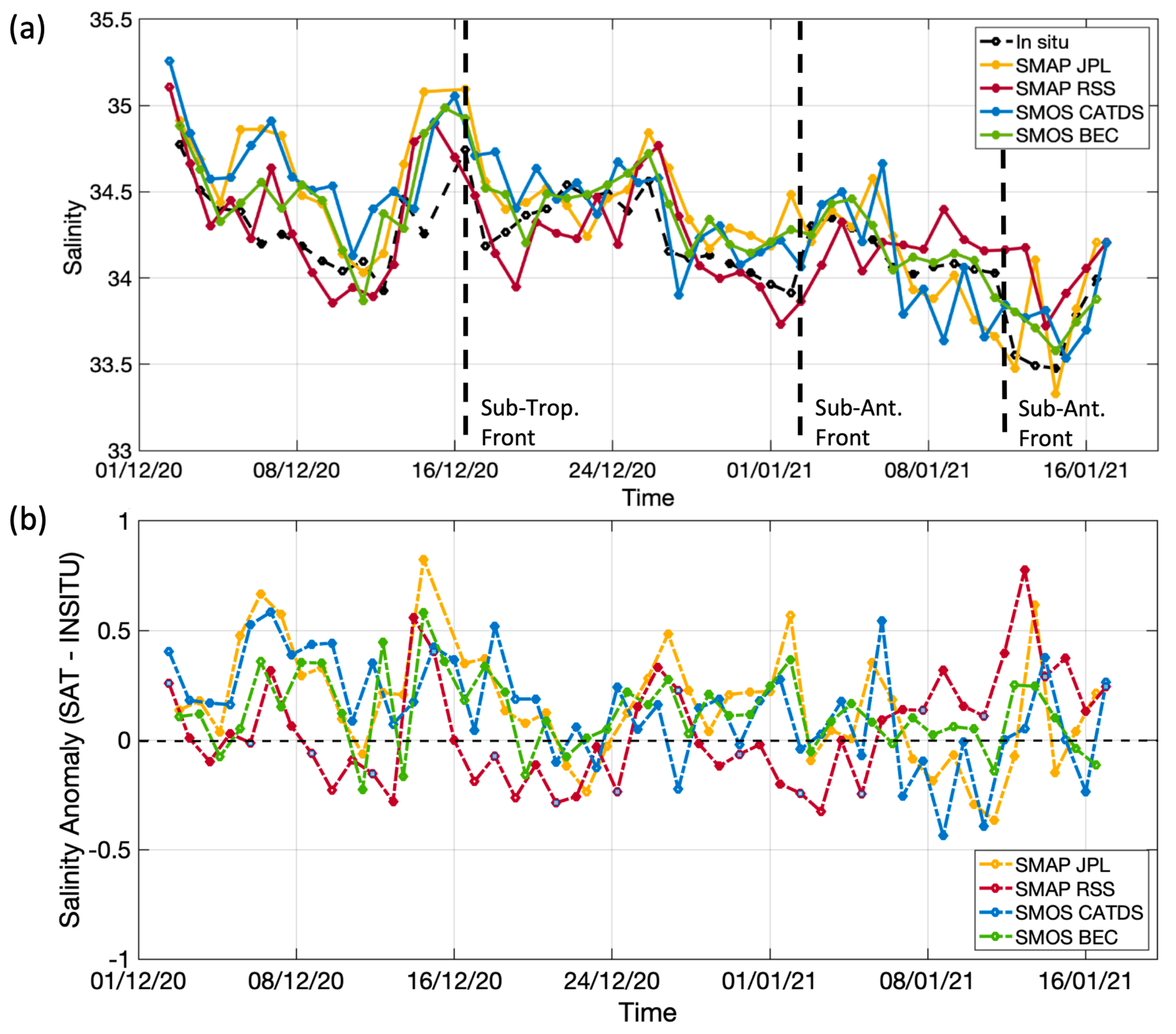
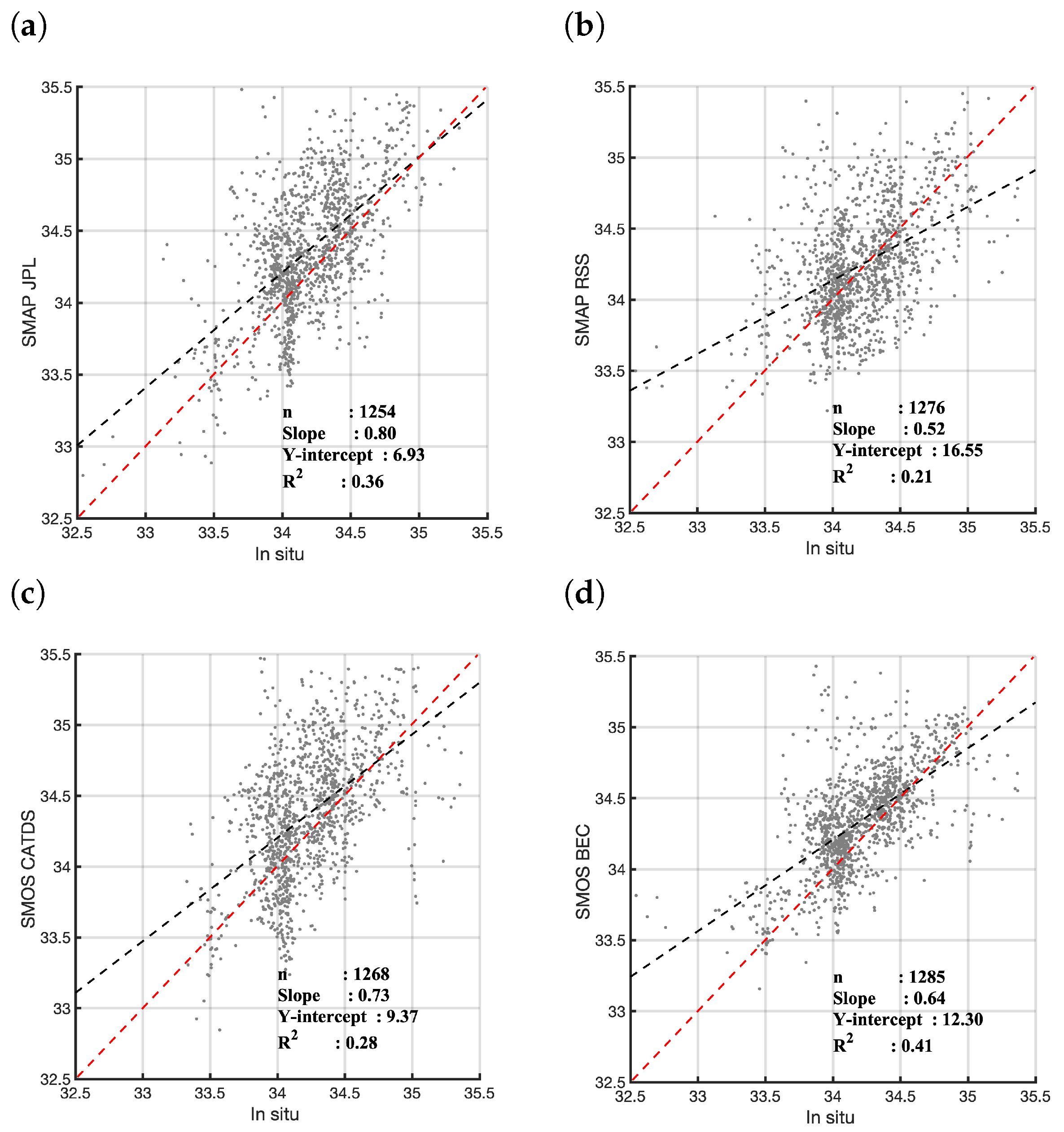
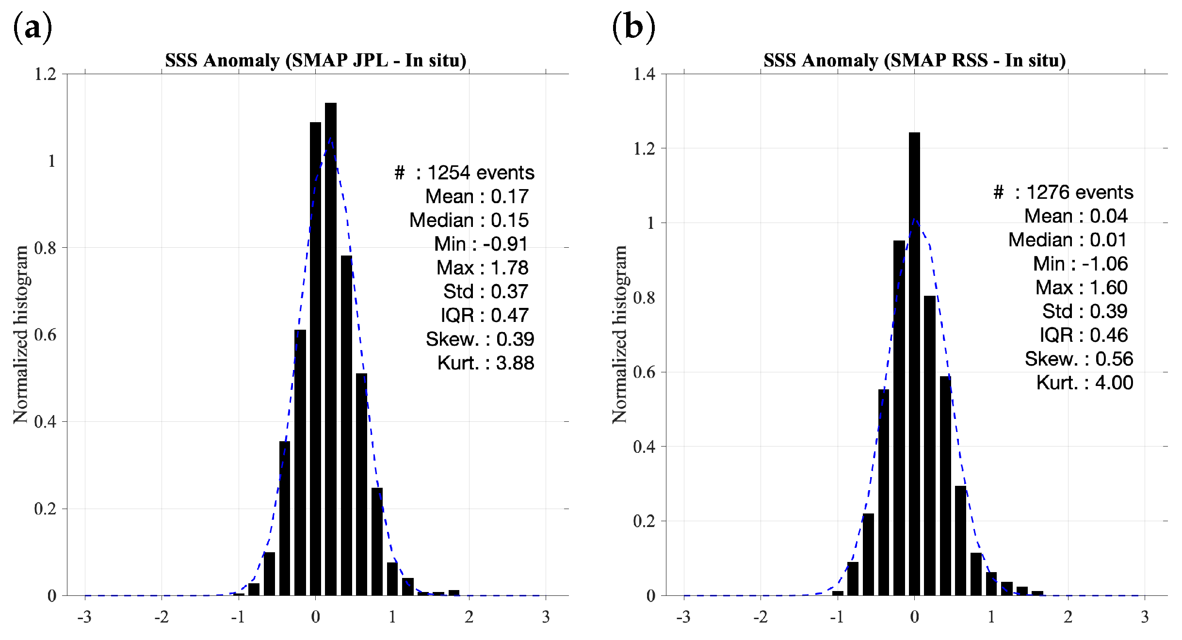
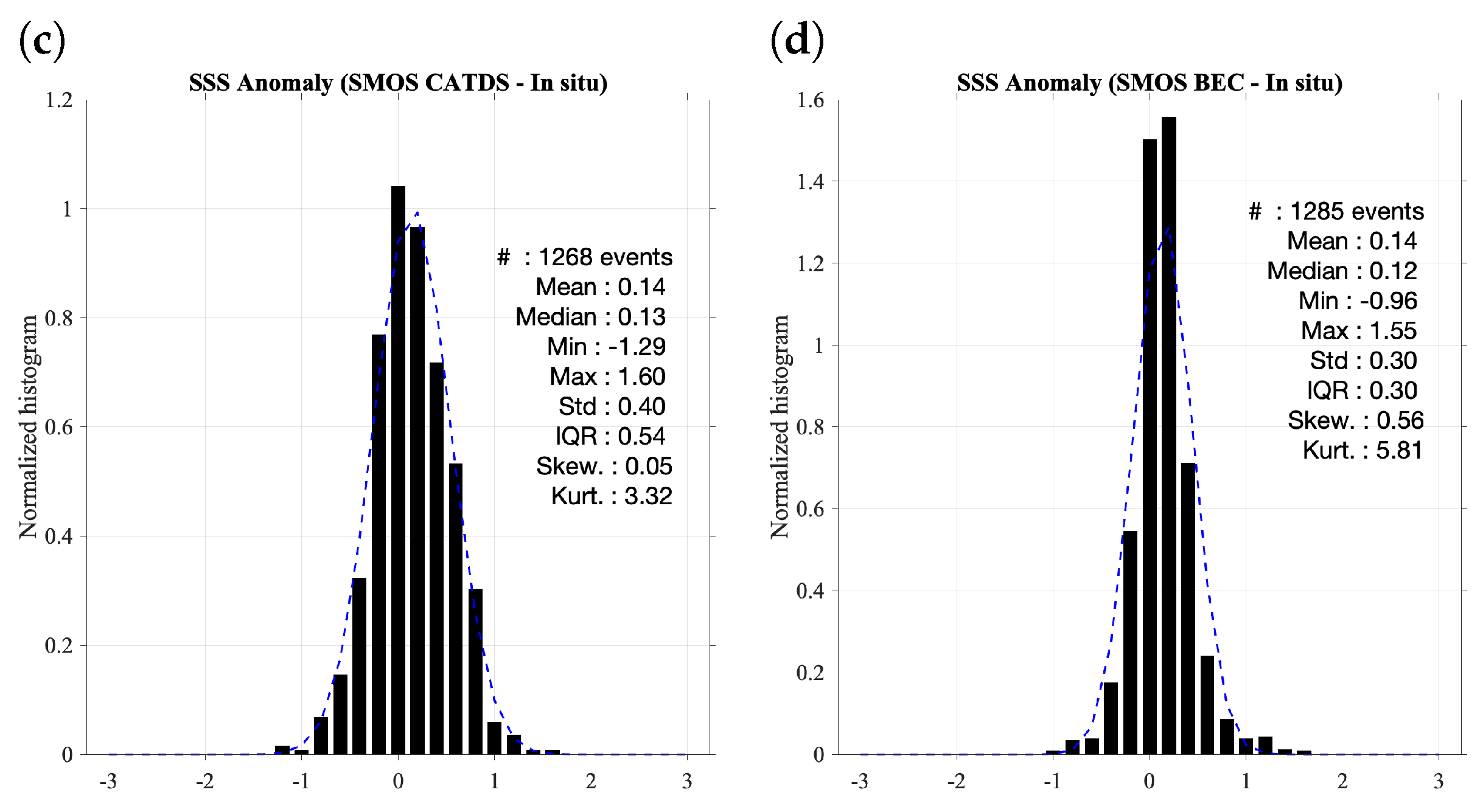
3.2. Validation of Satellite SSS

We used the Vendée Globe SSS in-situ measurements southern than 40° S to validate the four satellite SSS products in the sub-Antartic zone. We compared four time-space composite satellite products (so-called Level 3): SMAP JPL, SMAP RSS, SMOS CATDS and SMOS BEC. Each SSS product presents some differences in missing data close to ice edge close to Antarctica, and different levels of noise (changes of navy blue and cyan colors in Figure 9). It seems that the SMOS BEC product is less affected by noise but has less data coverage. All satellite SSS products are able to represent the saltiest Atlantic ocean compared to the Pacific and the Indian Ocean in the subtropical zone.
The Antarctic coast extends further North between 0 and 180° East (between Good Hope cape and Leeuwin cape) bringing colder waters to the Indian Ocean than to the Pacific ocean. Because of that, colder and fresher water rises northward in the Indian Ocean, as ice edge also extend further North. SMOS BEC and SMAP RSS products represents well this characteristic, even if the later seems to be more affected by noise. All four products depicted the subtropical front. Circumpolar current interacts with the continent landmass only in Patagonia, where all the products represent the Humboldt current transporting freshwater to the equator along the Chilean coast, and the Falklands current to the north, while the Brazil current brings warmer and saltier water to the south along Argentinian coast.
The match-up was performed after filtering the input in-situ data and by co-localising the in-situ SSS measurements into the spatio-temporal grid of satellite products. To avoid error representation due to differences in the spatial and temporal sampling, VG2020 SSS data have been averaged into the spatio-temporal grid of the satellite products (daily and 0.25 degree grid). For high-spatial resolution in-situ SSS measurements such as the Vendée Globe SSS data, this match-up procedure minimizes the spatial representation uncertainty when comparing to the lower spatial resolution of the satellite SSS product. The internal variability of filtered VG2020 data inside the satellite grid is computed as the STD of VG2020 data inside the spatio-temporal grid of the satellite products. The STD is in average 0.06 psu with maximum values of 0.44 psu in frontal and continental affected areas.
When analysing the time series south of 40° S of the VG2020 SSS filtered data and the averaged VG2020 SSS data (Figure 10), we can observe that the original high-frequency sampling provides information on the sub mesoscale variability not resolved at the remote sensed SSS grids. However, the typical SSS variability in the different oceans and the significant SSS changes when crossing fronts are still present in the averaged VG2020 SSS data.
Once the co-localization is performed, we analyse the difference between the satellite and co-localized in-situ SSS ( Δ S S S = S S S S A T S S S I n s i t u ). Time series of daily mean of in-situ and satellite SSS and of their difference ( Δ S S S ) are shown in Figure 11. The time series of the daily SSS mean estimated southern of 40° S for SMAP JPL (in yellow), SMAP RSS (in red), SMOS-CATDS (in blue), SMOS BEC (in green) products and the co-localized Vendée Globe in-situ dataset (in black) are shown in Figure 11a. Their anomaly with respect to the averaged VG2020 SSS data ( Δ S S S ) is showed in Figure 11b. We observe that the match-up pairs over the Sub-Antarctic region exhibit typical anomalies from −0.5 to 0.8 psu, with lower anomalies for the SMOS BEC product. Typical in-situ SSS variability south of 40° S (sub-Antarctic and sub-tropical fronts, glacier melting) is in general detected by all satellite products.
Figure 12 shows the scatterplots of satellite SSS (y-axis) versus VG2020 SSS (x-axis) below 40° S. For each plot, the red dashed line shows the x = y. The black dashed line indicates the linear fit through the data cloud. The number match-up pairs n, the slope and R2 coefficients of the linear fit are indicated in each plots. Better correlations with VG2020 data are found for SMOS BEC (R = 0.64), followed by SMAP JPL (R = 0.60), SMOS CATDS (R = 0.53) and SMAP RSS (R = 0.45).
In Figure 13, we represent the histograms of the SSS anomalies match-ups that correspond to the Δ S S S distributions for the four satellite products. Each plot includes among other statistics the standard deviation (STD), the mean, the median, the minimum and maximum bias between satellite products and averaged VG2020 SSS data. Better accuracy is found when using SMOS BEC product (STD = 0.30 psu), and lower accuracy using SMOS CATDS product (STD = 0.40 psu). SMAP SSS products presented STD = 0.37 and 0.39 for JPL and RSS products respectively. The lower bias is found for SMAP RSS procuct (median = 0.01 psu), followed by SMOS BEC (median = 0.12 psu), SMOS CATDS (median = 0.13 psu), and SMAP JPL (median = 0.15 psu).

4. Conclusions

The in-situ data obtained with the One Ocean One Planet boat competing in the Vendée Globe race are presented in this study. Results show that reliable data can be obtained for scientific purposes using vessels competing in round-the-world regattas. The data were thoroughly filtered and used to identify the typical sub-Antarctic oceanic features. Signatures of melting-affected regions, as well as sub-tropical and sub-polar fronts, were clearly recognized. Even if some parts of the race vessel measurements exhibit foam and air particle effects that must be filtered, they still represent a source of real surface information that is extremely beneficial as a sea-truth reference as well as for climatological studies.
For instance, this new data collection proves to be of great use for the validation of L-band SSS products in the Southern Ocean using ESA and NASA SSS missions. Because the race route includes infrequently sampled locations, the data gathered by One Ocean One Planet are very relevant for the validation of remotely sensed products. This provides significant insight into the assessment of the satellite SSS products since satellite data are typically validated using Argo data, despite the fact that their shallowest observations are between 2 and 10 m depth, which may overlook surface features observed by satellites. The values obtained with the One Ocean One Planet boat are much shallower (60 cm depth) which is closer to satellite observations than the Argo data.
The present contribution to ocean surface salinity data gathered within the Vendée Globe has been successfully used to validate satellite SSS products for the Southern Ocean, provided by ESA and NASA SSS missions. During the period that the regatta sailed south of 40S (3 December 2020–18 January 2021), the satellite products revealed average differences of 0.01–0.15 psu and a range of 0.3–0.4 psu standard deviation with respect to satellite observations.
These results are a step forward to analyzing the evolution of ocean salinity in sub-Antarctic zones and the impact of changes in the ice extent around Antarctica. Having periodic in-situ measurements in the sub Antarctic zone should allow us to analyze the impacts of the ice extent changes in the Antarctica and in the sub Antarctic zone. The study reveals the interest in data recording efforts through competing boats in the periodic round world races to contribute to ocean scientific knowledge. This novel research proves that the regatta’s various vessels competing in Vendée Globe race every four years can be equipped for research in the future.

Author Contributions

Conceptualization, M.U., N.H., J.S. (Joaquin Salvador), J.S. (Jordi Salat); methodology, J.S. (Jordi Salat), M.U., N.H.; software, M.U., J.S. (Jordi Salat), N.H., S.G.; validation, M.U., S.G. and N.H.; investigation, M.U., J.S. (Jordi Salat), and N.H.; data curation, J.S. (Jordi Salat), M.U., S.G., J.S. (Joaquin Salvador); writing—original draft preparation, M.U., J.S. (Jordi Salat), J.S. (Joaquin Salvador); writing—review and editing, N.H., J.S. (Jordi Salat), E.O., C.G., S.G.; funding acquisition, M.U., J.S. (Jordi Salat), E.O. and C.G. All authors have read and agreed to the published version of the manuscript.

Funding

This work has been carried out thanks to European Union’s Horizon 2020 research and innovation programme under the Marie Skłodowska-Curie Grant Agreement No. 840374. We also received funding from the Spanish government through the “Severo Ochoa Centre of Excellence” accreditation (CEX2019-000928-S).

Institutional Review Board Statement

Not applicable.

Informed Consent Statement

Not applicable.

Data Availability Statement

In-situ filtered data are available on demand by contacting the BEC Support Desk: [email protected].

Acknowledgments

This work represents a contribution to the CSIC Thematic Interdisciplinary Platform PTI POLARCSIC and PTI TELEDETECT.

Conflicts of Interest

The authors declare no conflict of interest.

References

  1. Tang, W.; Yueh, S.; Yang, D.; Fore, A.; Hayashi, A.; Lee, T.; Fournier, S.; Holt, B. The potential and challenges of using Soil Moisture Active Passive (SMAP) sea surface salinity to monitor Arctic Ocean freshwater changes. Remote Sens. 2018, 10, 869. [Google Scholar] [CrossRef] [Green Version]
  2. Olmedo, E.; Gabarró, C.; González-Gambau, V.; Martínez, J.; Ballabrera-Poy, J.; Turiel, A.; Portabella, M.; Fournier, S.; Lee, T. Seven years of SMOS sea surface salinity at high latitudes: Variability in Arctic and Sub-Arctic regions. Remote Sens. 2018, 10, 1772. [Google Scholar] [CrossRef] [Green Version]
  3. Umbert, M.; Gabarro, C.; Olmedo, E.; Gonçalves-Araujo, R.; Guimbard, S.; Martinez, J. Using Remotely Sensed Sea Surface Salinity and Colored Detrital Matter to Characterize Freshened Surface Layers in the Kara and Laptev Seas during the Ice-Free Season. Remote Sens. 2021, 13, 3828. [Google Scholar] [CrossRef]
  4. Fournier, S.; Lee, T.; Wang, X.; Armitage, T.W.; Wang, O.; Fukumori, I.; Kwok, R. Sea surface salinity as a proxy for Arctic Ocean freshwater changes. J. Geophys. Res. Ocean. 2020, 125, e2020JC016110. [Google Scholar] [CrossRef]
  5. Martínez, J.; Gabarró, C.; Turiel, A.; González-Gambau, V.; Umbert, M.; Hoareau, N.; González-Haro, C.; Olmedo, E.; Arias, M.; Catany, R.; et al. Improved BEC SMOS Arctic Sea surface salinity product v3. 1. Earth Syst. Sci. Data 2022, 14, 307–323. [Google Scholar] [CrossRef]
  6. Banks, C.J.; Gommenginger, C.P.; Srokosz, M.A.; Snaith, H.M. Validating SMOS ocean surface salinity in the Atlantic with Argo and operational ocean model data. IEEE Trans. Geosci. Remote Sens. 2012, 50, 1688–1702. [Google Scholar] [CrossRef]
  7. Tang, W.; Yueh, S.H.; Fore, A.G.; Hayashi, A. Validation of A quarius sea surface salinity with in situ measurements from A rgo floats and moored buoys. J. Geophys. Res. Ocean. 2014, 119, 6171–6189. [Google Scholar] [CrossRef]
  8. Salat, J.; Umbert, M.; Ballabrera-Poy, J.; Fernández, P.; Salvador, K.; Martínez, J. The contribution of the Barcelona World Race to improved ocean surface information. A validation of the SMOS remotely sensed salinity. Contrib. Sci. 2013, 9, 89–100. [Google Scholar]
  9. Gourrion, J.; Szekely, T.; Killick, R.; Owens, B.; Reverdin, G.; Chapron, B. Improved statistical method for quality control of hydrographic observations. J. Atmos. Ocean. Technol. 2020, 37, 789–806. [Google Scholar] [CrossRef]
  10. Cunningham, S.; Alderson, S.; King, B.; Brandon, M. Transport and variability of the Antarctic circumpolar current in drake passage. J. Geophys. Res. Ocean. 2003, 108. [Google Scholar] [CrossRef] [Green Version]
  11. Donohue, K.; Tracey, K.; Watts, D.; Chidichimo, M.P.; Chereskin, T. Mean antarctic circumpolar current transport measured in drake passage. Geophys. Res. Lett. 2016, 43, 11760–11767. [Google Scholar] [CrossRef] [Green Version]
  12. Orsi, A.H.; Whitworth, T.; Nowling, W. On the meridional extent and fronts of the Antarctic Circumpolar Current. Deep Sea Res. Ser. I 1995, 42, 641–673. [Google Scholar] [CrossRef]
  13. Sokolov, S.; Rintoul, S.R. Circumpolar structure and distribution of the Antarctic Circumpolar Current fronts: 2. Variability and relationship to sea surface height. J. Geophys. Res. Ocean. 2009, 114. [Google Scholar] [CrossRef] [Green Version]
  14. Giglio, D.; Johnson, G.C. Subantarctic and polar fronts of the Antarctic Circumpolar Current and Southern Ocean heat and freshwater content variability: A view from Argo. J. Phys. Oceanogr. 2016, 46, 749–768. [Google Scholar] [CrossRef]
  15. Fore, A.G.; Yueh, S.H.; Tang, W.; Stiles, B.W.; Hayashi, A.K. Combined active/passive retrievals of ocean vector wind and sea surface salinity with SMAP. IEEE Trans. Geosci. Remote Sens. 2016, 54, 7396–7404. [Google Scholar] [CrossRef]
  16. Meissner, T.; Wentz, F.; Manaster, A.; Lindsley, R. Remote Sensing Systems SMAP Ocean Surface Salinities Level 3 Running 8-Day, Version 4.0 Validated Release; Remote Sensing Systems: Santa Rosa, CA, USA, 2019. [Google Scholar]
  17. Olmedo, E.; González-Haro, C.; Hoareau, N.; Umbert, M.; González-Gambau, V.; Martínez, J.; Gabarró, C.; Turiel, A. Nine years of SMOS sea surface salinity global maps at the Barcelona Expert Center. Earth Syst. Sci. Data 2021, 13, 857–888. [Google Scholar] [CrossRef]
  18. Boutin, J.; Vergely, J.L.; Marchand, S.; d’Amico, F.; Hasson, A.; Kolodziejczyk, N.; Reul, N.; Reverdin, G.; Vialard, J. New SMOS Sea Surface Salinity with reduced systematic errors and improved variability. Remote Sens. Environ. 2018, 214, 115–134. [Google Scholar] [CrossRef] [Green Version]
Figure 1. Sailing racer Dídac Costa onboard the One Planet One Ocean, an Open 60 sailing boat arriving to Les Sables d’Olonne after a world tour during the ninth edition of the Vendée Globe race. Image from www.vendeeglobe.org, last accessed on 5 August 2022, with copyright of Jean-Louis Carli-Alea.
Jmse 10 01078 g001
Figure 2. One Planet One Ocean trajectory during the 9th edition of Vendée Globe race. In red: TAS: Tasmania, CAPE G.H: Cape of Good Hope, CAPE HOR: Cape of Hornos, CAPE L.: Cape of Leeuwin, and the Nemo Point (124.39° W, 48.87° S) is indicated with a red cross.
Jmse 10 01078 g002
Figure 3. Position of conductivity-temperature sensor that was installed onboard the One Ocean One Planet boat.
Jmse 10 01078 g003
Figure 4. Temporal evolution of raw and filtered salinity data (a) and temperature (b) along the sailing race trajectory.
Jmse 10 01078 g004
Figure 5. (a) Salinity (psu), (b) temperature (°C), (c) density (kg/m3) and (d) velocity (knots) along the trajectory.
Jmse 10 01078 g005
Figure 6. Temperature−Salinity diagram of surface in-situ filtered data showing the water masses: Southern Indian Waters (SIW), Southern Pacific Waters (SPW), SubAntarctic Waters (SAW) and South Atlantic Central Waters (SAW), and fronts found along the trajectory. Isopycnals ( σ θ ) are shown and colours correspond to the longitude (°) as shown in the right side colourbar.
Jmse 10 01078 g006
Figure 7. (a) Temperature−Salinity diagram using the filtered in-situ data in the Pacific Ocean (colors indicate the longitude (°) and contours represent the ispycnals σ θ ). (b) Salinity (psu) and (c) temperature (°C) recorded in the Pacific Ocean.
Jmse 10 01078 g007
Figure 8. (a) Temperature−Salinity diagram using the filtered in-situ data along the South Patagonia-Cape Horn (colors indicate the longitude (°) and contours represent the isopycnals σ θ ). (b) Salinity (psu) and (c) temperature (°C) recorded in the South Patagonia-Cape Horn area.
Jmse 10 01078 g008
Figure 9. Example of SSS remotely sensed products for the 10 January 2021. (a) SMAP JPL; (b) SMAP RSS; (c) SMOS CATDS and; (d) SMOS BEC. The black line indicates the trajectory of One Ocean One Planet ship and the red star its position on 10 January 2021.
Jmse 10 01078 g009
Figure 10. Original high-frequency VG2020 salinity measurements (black dots) and the collocated VG2020 SSS data to satellite 0.25, daily grid (red diamonds) southern than 40° S.
Jmse 10 01078 g010
Figure 11. (a) Temporal evolution of daily-mean co-localized VG2020 measurements and the four satellite products along the vessel trajectory; (b) SSS anomaly between satellite products and VG2020 SSS data.
Jmse 10 01078 g011
Figure 12. Scatter plots between VG2020 SSS and satellite SSS data for (a) SMAP JPL, (b) SMAP RSS, (c) SMOS CATDS, (d) SMOS BEC. The number of match-up pairs (n), slope, y−intercept and R2 coefficients of the linear fit are indicated in each plot.
Jmse 10 01078 g012
Figure 13. Histograms of SSS anomalies (satellite−in-situ) using (a) SMAP JPL, (b) SMAP RSS, (c) SMOS CATDS, (d) SMOS BEC.
Jmse 10 01078 g013aJmse 10 01078 g013b
Publisher’s Note: MDPI stays neutral with regard to jurisdictional claims in published maps and institutional affiliations.

