A Real-Time Ship Detector via a Common Camera

Abstract

Advanced radars and satellites, suitable for remote monitoring, inappropriately reach the economical requirements of short-range detection. Compared with far-sightedness skills, common visible-light sensors offer more ample features conducive to distinguishing the classes. Therefore, ship detection based on visible-light cameras should cooperate with remote detection technologies. However, compared with detectors applied in inland transportation, the lack of fast ship detectors, detecting multiple ship classes, is non-negligible. To fill this gap, we propose a real-time ship detector based on fast U-Net and remapping attention (FRSD) via a common camera. The fast U-Net offered compresses features in the channel dimension to decrease the number of training parameters. The remapping attention introduced boosts the performance in various rain–fog weather conditions while maintaining the real-time speed. The ship dataset proposed contains more than 20,000 samples, alleviating the lack of ship datasets containing various classes. Data augmentation of the cross-background is especially proposed to further promote the diversity of the detecting background. In addition, the rain–fog dataset proposed, containing more than 500 rain–fog images, simulates various marine rain–fog scenarios and soaks the testing image to validate the robustness of ship detectors. Experiments demonstrate that FRSD performs relatively robustly and detects 9 classes with an mAP of more than 83%, reaching a state-of-the-art level.

1. Introduction

Considering the marine environment and the detecting sphere, various radars or optical satellites are the primary resources for ship detection. Regardless of the classification, advanced radars and satellites detect ships by extraordinary resolution images containing ample information, which is helpful to detect ships in a remote range. Nevertheless, advanced military radars, suitable for far detection, hardly economically maintain real-time performance in the middle-range or below detection, considering the suitability of remote detection and material deformation [1,2] raised by long-term operations. Although synthetic aperture radars (SAR) undertake all-day detection tasks and the locating accuracy is practical, classifying the ship classes is in a weak position due to the relatively single features offered [3,4]. Optic satellites can offer ample features to distinguish the classes, while ultra long-distance detection is susceptible to cloud and fog. In addition, satellites do not meet the requirement of real-time speed in an economical way [5,6] due to high maintenance and replacement costs. For civilian radar and infrared imaging technology, the limited detection capacity raised by unideal weather conditions is non-negligible [7,8]. The images offered from the civilian radars and infrared sensors have relatively single features compared with the visible-light sensors. Therefore, it is challenging to meet the real-time and appropriate requirements of ship detection with a single skill. Compared with the detection skills above, although ship detection utilising the standard camera of visible-light sensors is susceptible to rain and fog, visible-light sensors economically meet the the relatively close range detection requirement under ideal weather conditions. In addition, the images obtained by visible-light sensors are far more abundant, which is suitable to distinguish the ship classes [9]. Comprehensively, ship detection based on visible-light sensors can cooperate with remote detection technologies via compensation.

The common target detectors contain conventional and modern detectors. Conventional detectors tend to be dependent on manual interference and have relatively little generalisation in various conditions or a large redundancy in window calculation [10]. Modern detectors, mainly consisting of CNNs, are increasingly mounting, owing to the impressive performance in the computer version. Most modern target detectors are categorised into two kinds, two-stage and one-stage detectors. The main classic two-stage detectors, whose workflow is divided into classifying and localizing regression, contain the R-CNN series [11,12,13], RepPoints [14], etc. R-CNN series detectors are based on predesigned anchors, in contrast, RepPoints is the anchor-free detector. The representative one-stage detectors, whose workflow unifies the classifying processing and localizing regression into one regression, contain SSD [15], YOLO series [16,17,18,19,20], EfficientDet [21], etc. The one-stage detectors tend to better balance inference and accuracy than two-stage detectors. In particular, YOLOv5s [20] (the light model of YOLOv5) has fewer parameters and relatively fast inference, which becomes one basement of potential ship detectors. However, there is a relative lack of ship detectors that detect multiple ship classes with real-time inference by visible cameras. Common target detectors are not directly applicable to ship detection, owing to the uniqueness of marine transportation. There is a serious lack of open datasets for intelligent maritime transport compared with KITTI [22], Torontocity [23], and RobotCar [24], which are suitable for inland transportation. Although an enhanced ship detector [9] based on YOLOv3 detects multi-class ships, the detecting background lacks the consideration of aerial scenes, and the corresponding application is suitable for shore-based detection. In addition, the testing datasets of COCO [25] and VOC [26] tend to validate detectors in an ideal state, leading to the fact that the robustness of ship detectors is rarely validated in actual application scenarios.

This paper considers the common visible-light camera to establish the low–high cooperation with radars or satellites suitable for far-sightedness. To pursue the ship detector detecting various ship classes and validate algorithms quantitatively in several rain–fog soaking degrees, our contributions are summarised as follows:

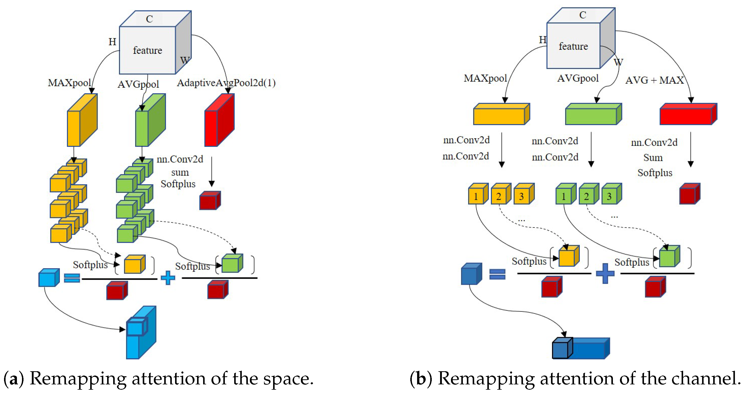
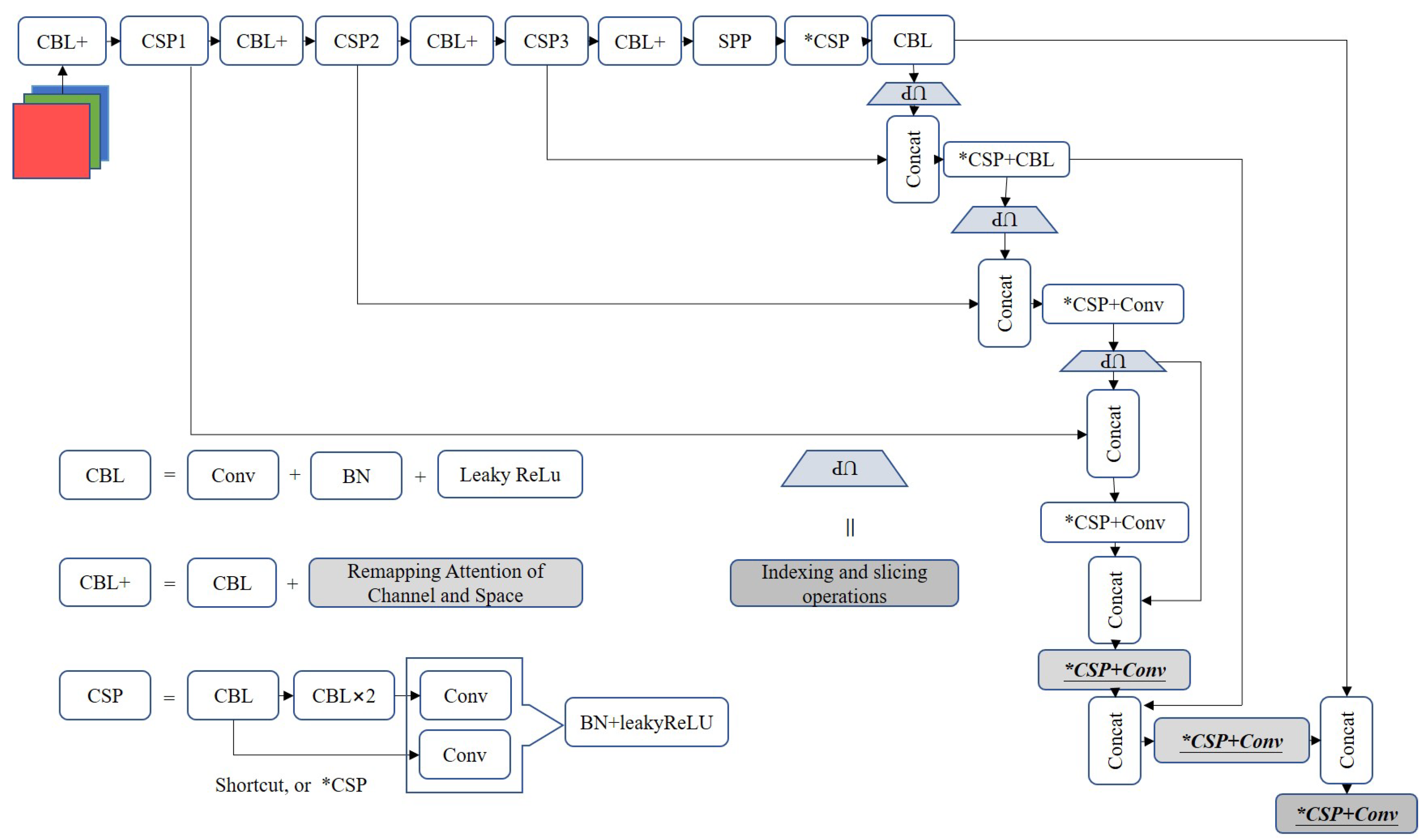
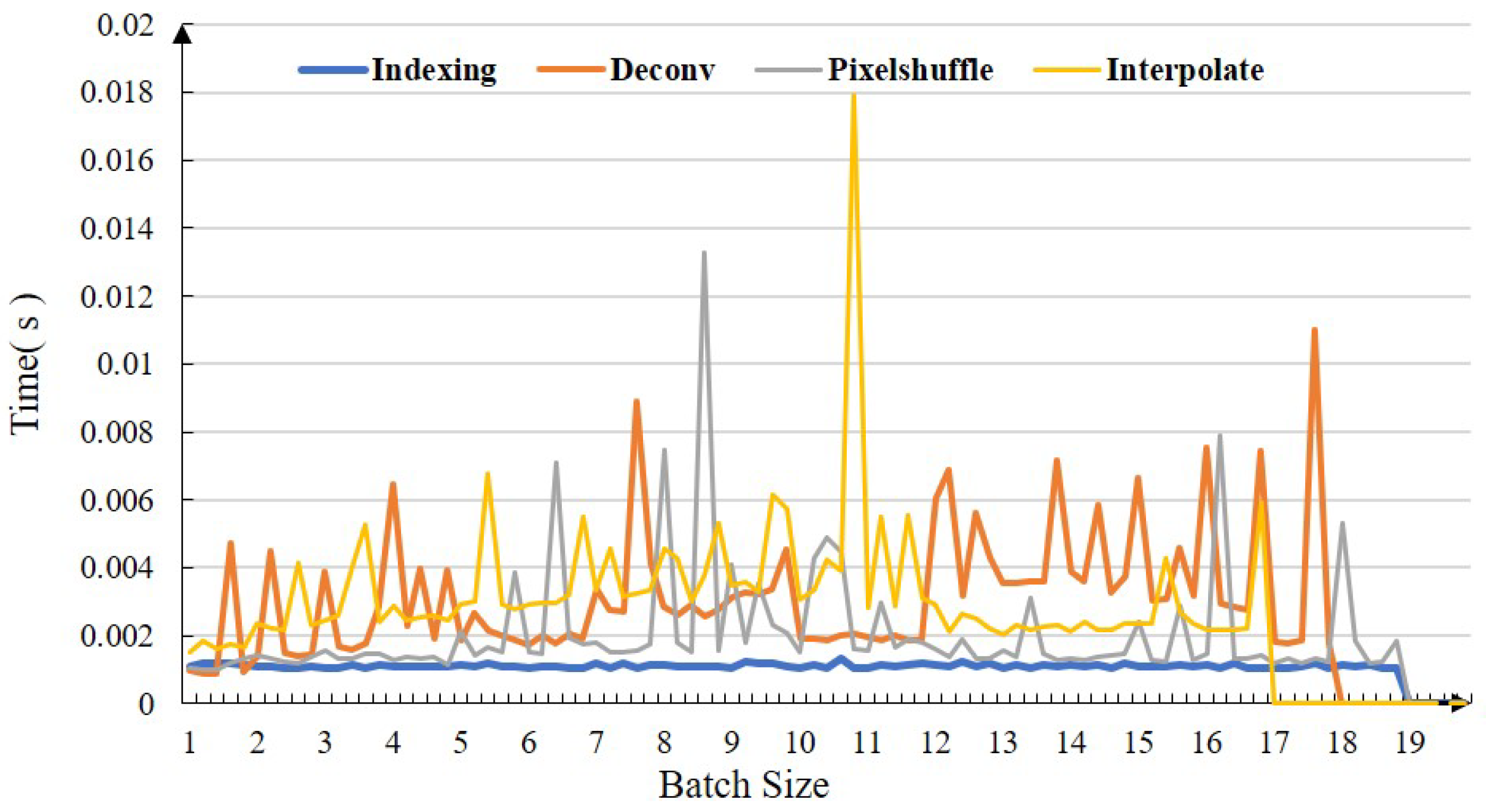
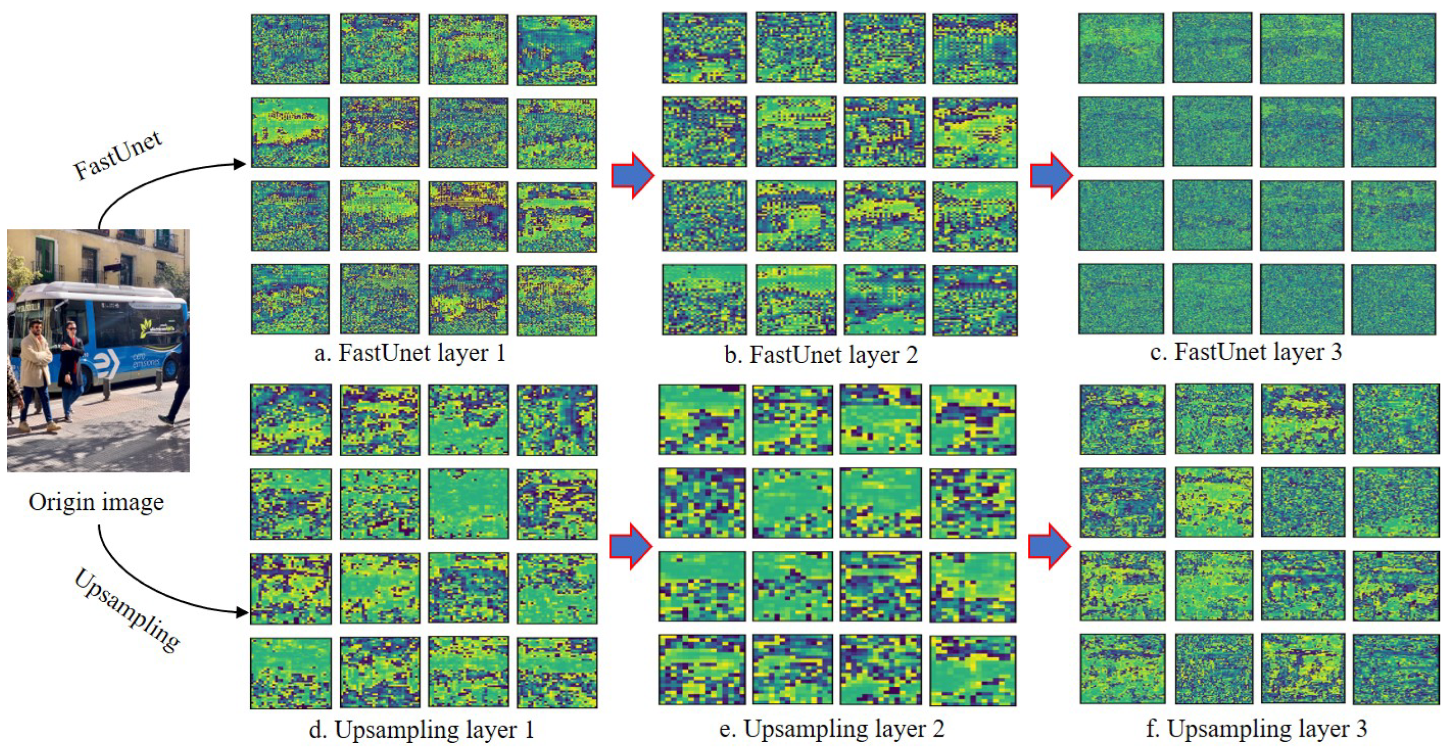
• We propose a real-time ship detector which is built on fast U-Net and remapping attention proposed. The fast U-Net offered adopts pixel period insertion to prompt the inference when multiple testing batches are set and decrease the number of training parameters. Remapping attention is specifically introduced to remap global features to local calculations, which is conducive to increasing the robustness in actual rain and fog scenes;
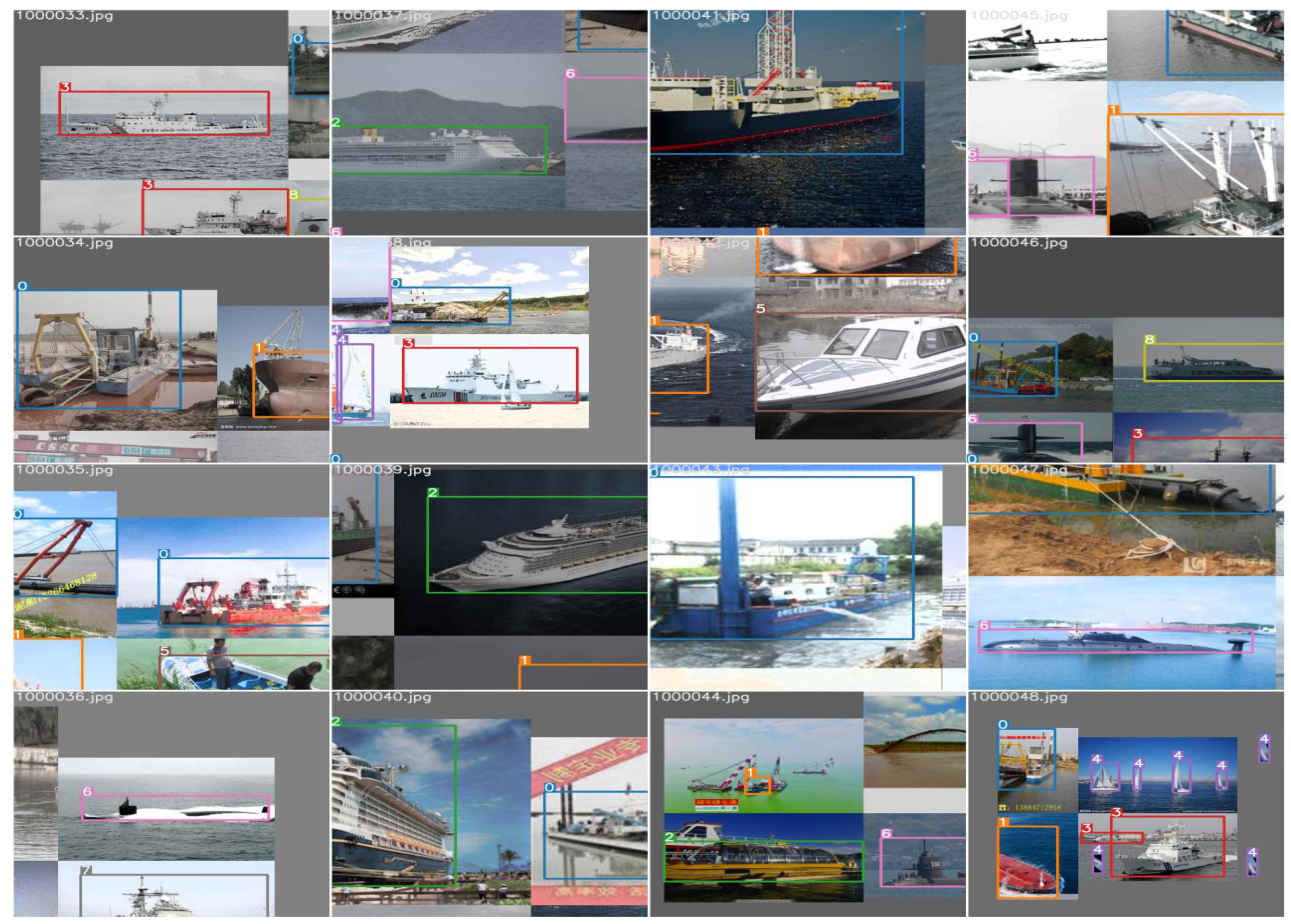
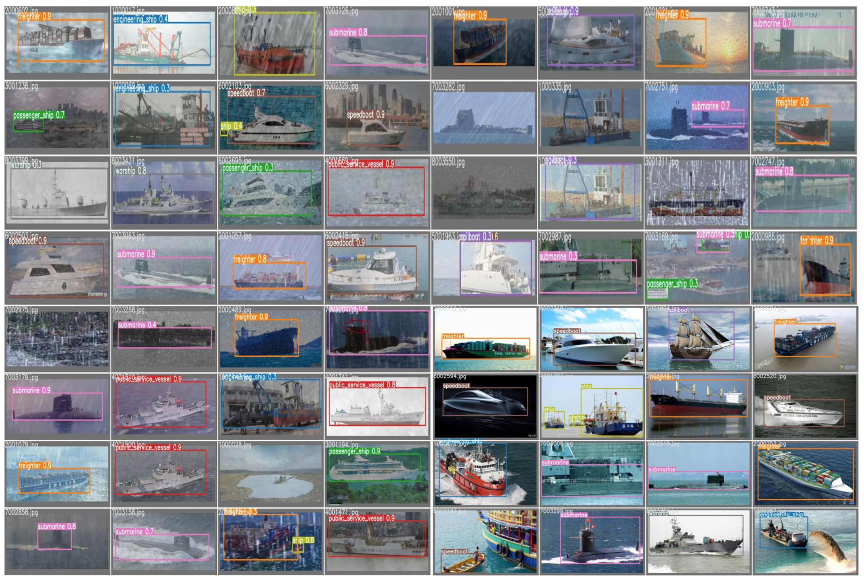
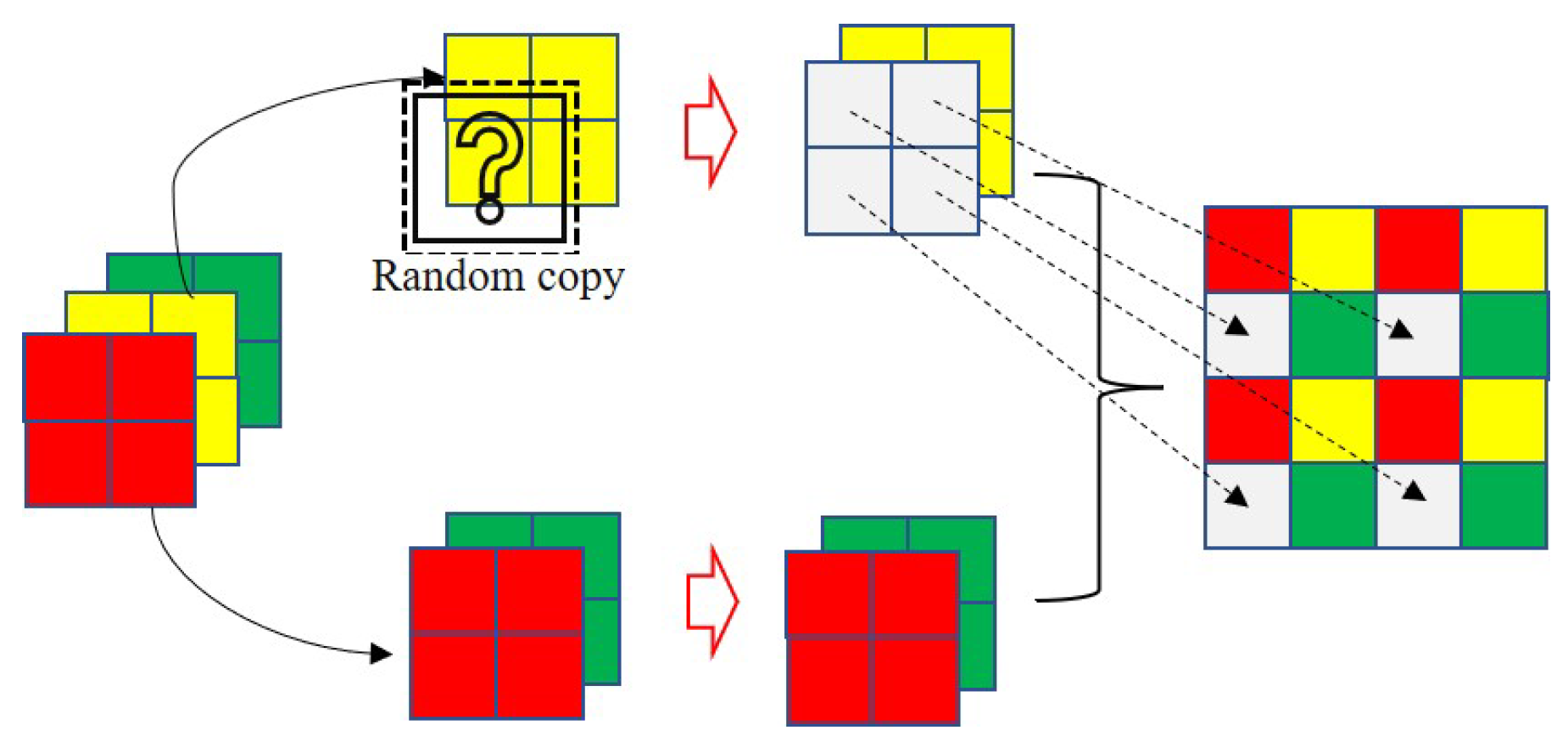
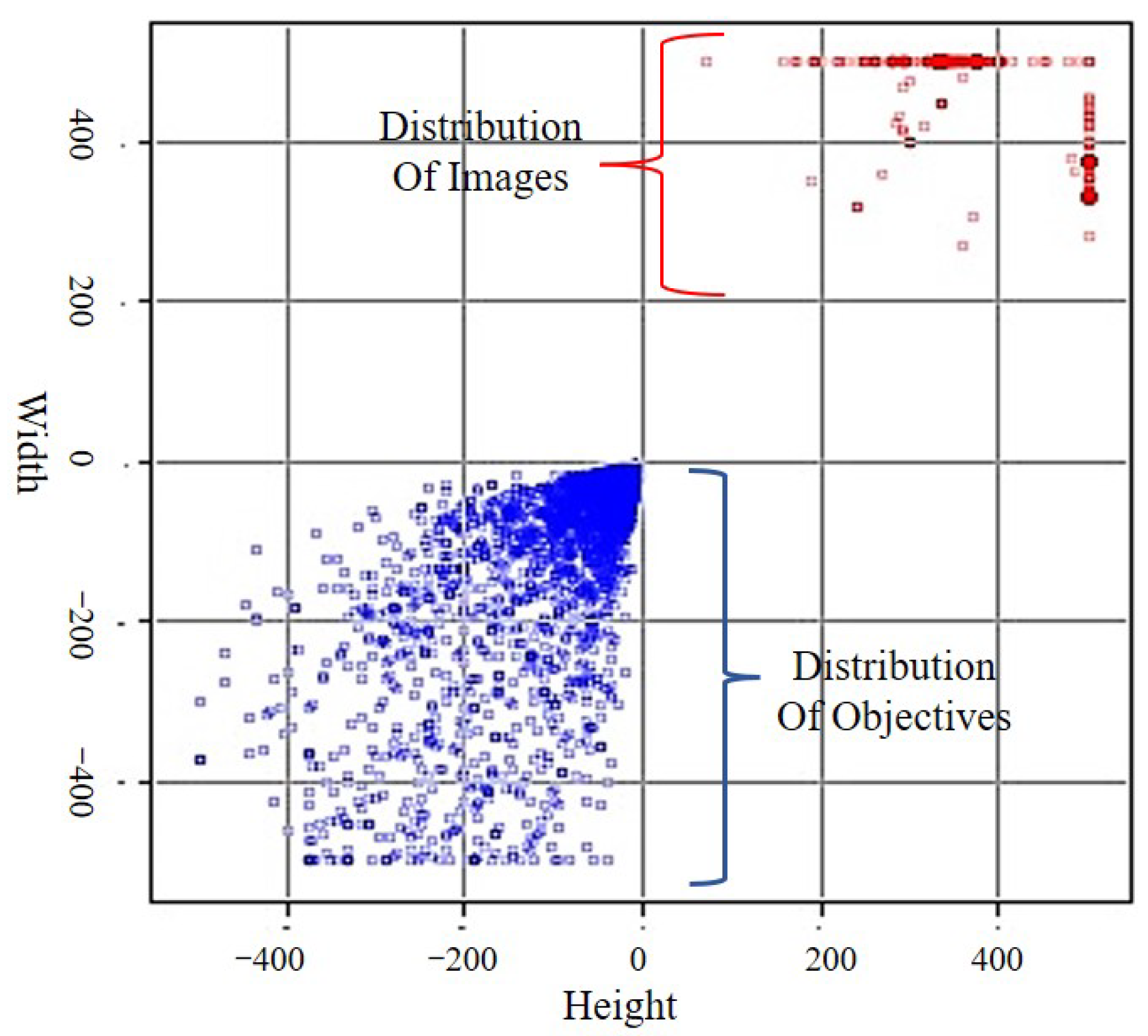
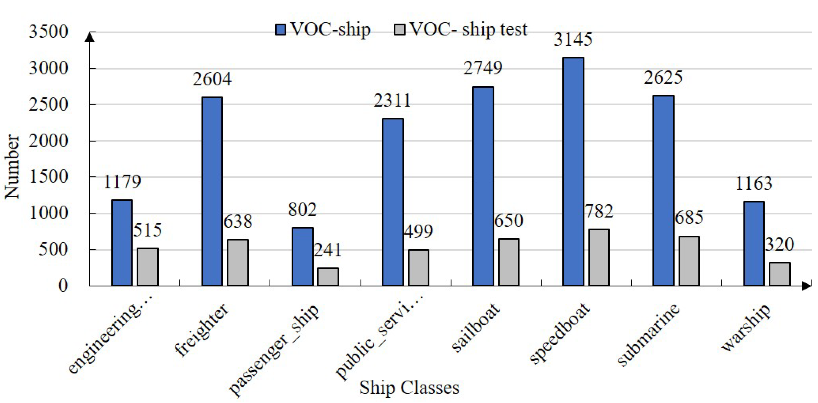
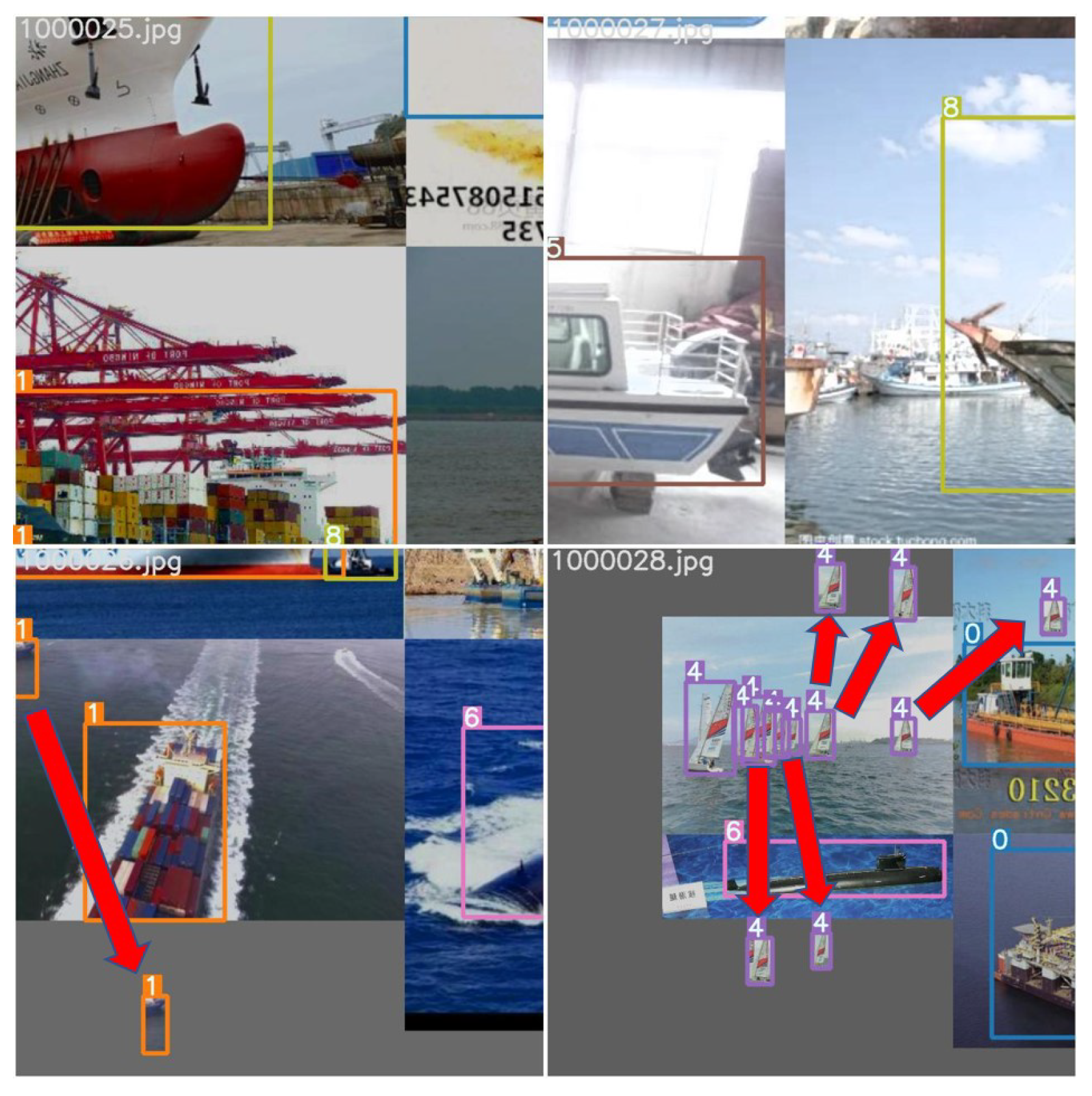
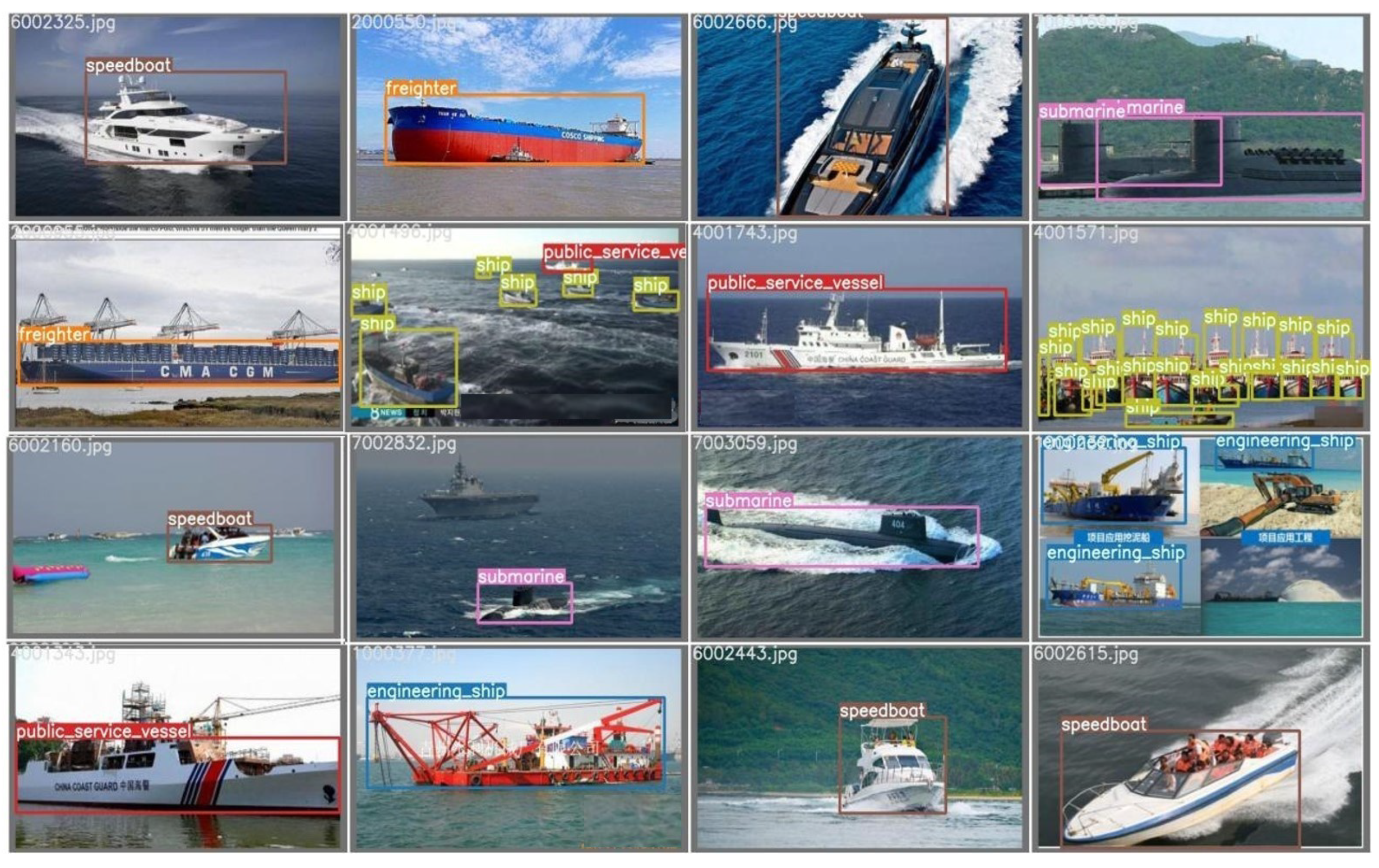
• We offer a ship dataset containing more than 14,000 images and data augmentation for the diversity of detecting backgrounds. The ship dataset provided alleviates the dataset’s lack of multiple ship classes. The data augmentation of the crossing-background randomly selects the targets copied to the new background, promoting the value of ship datasets and background diversity;
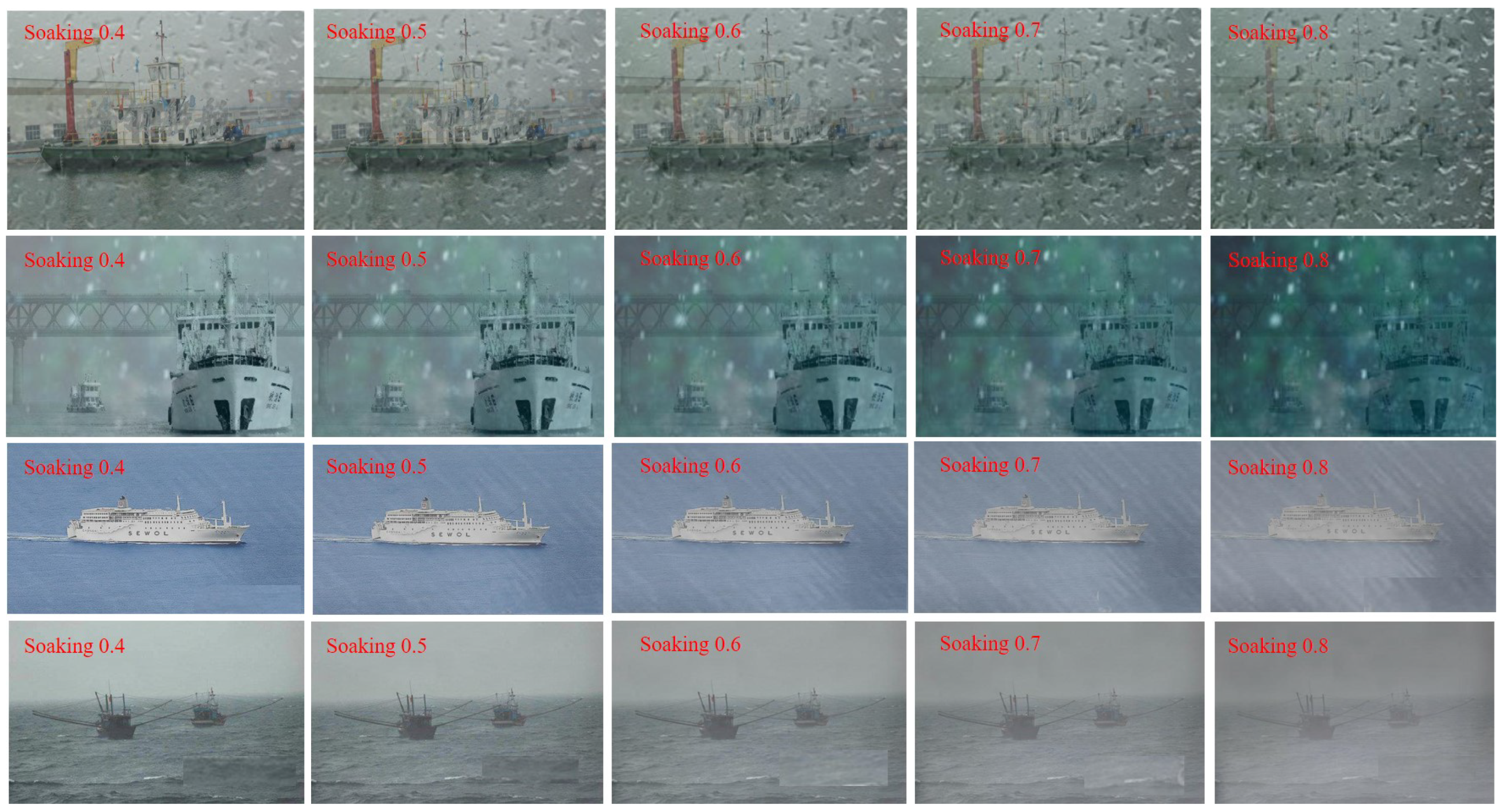
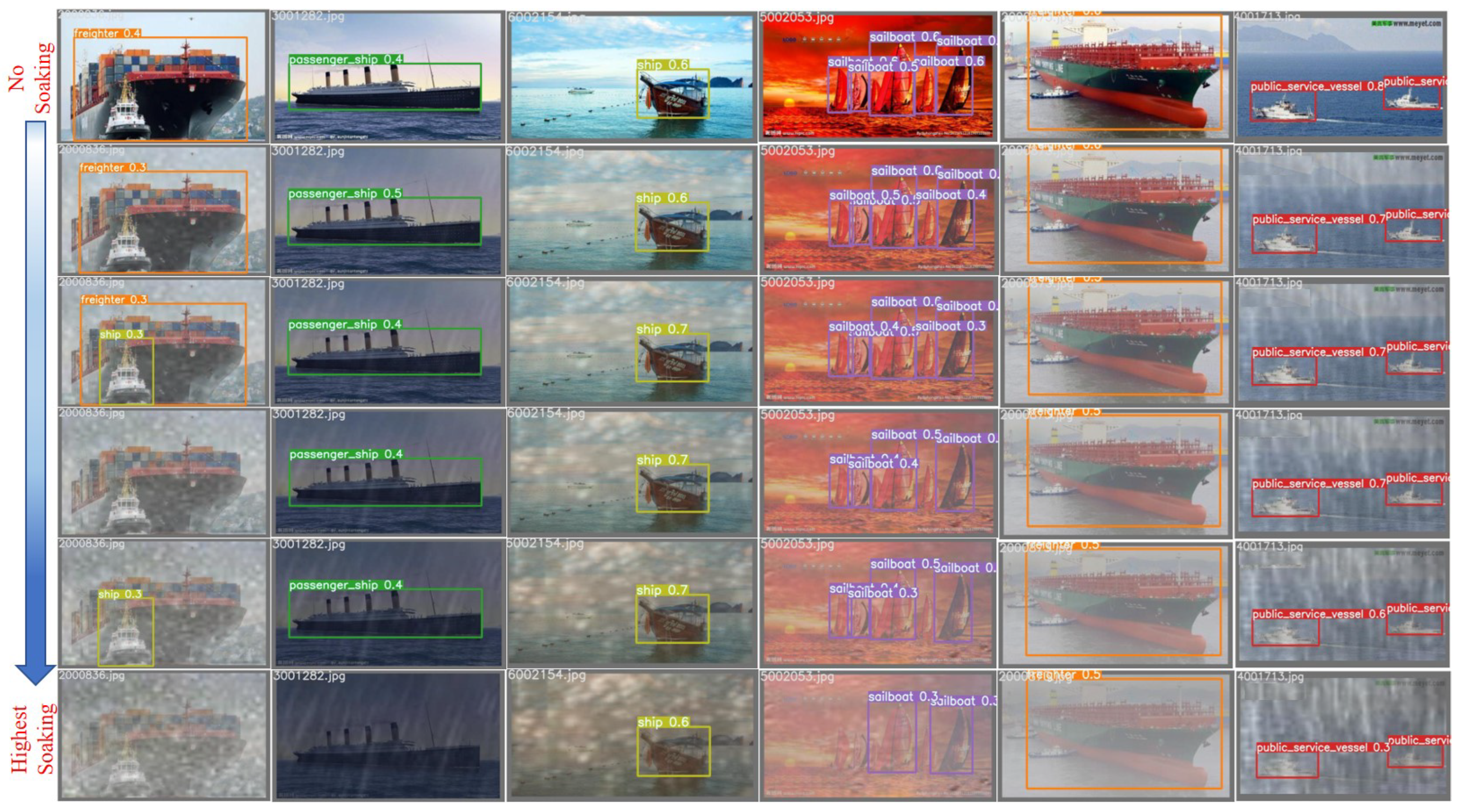
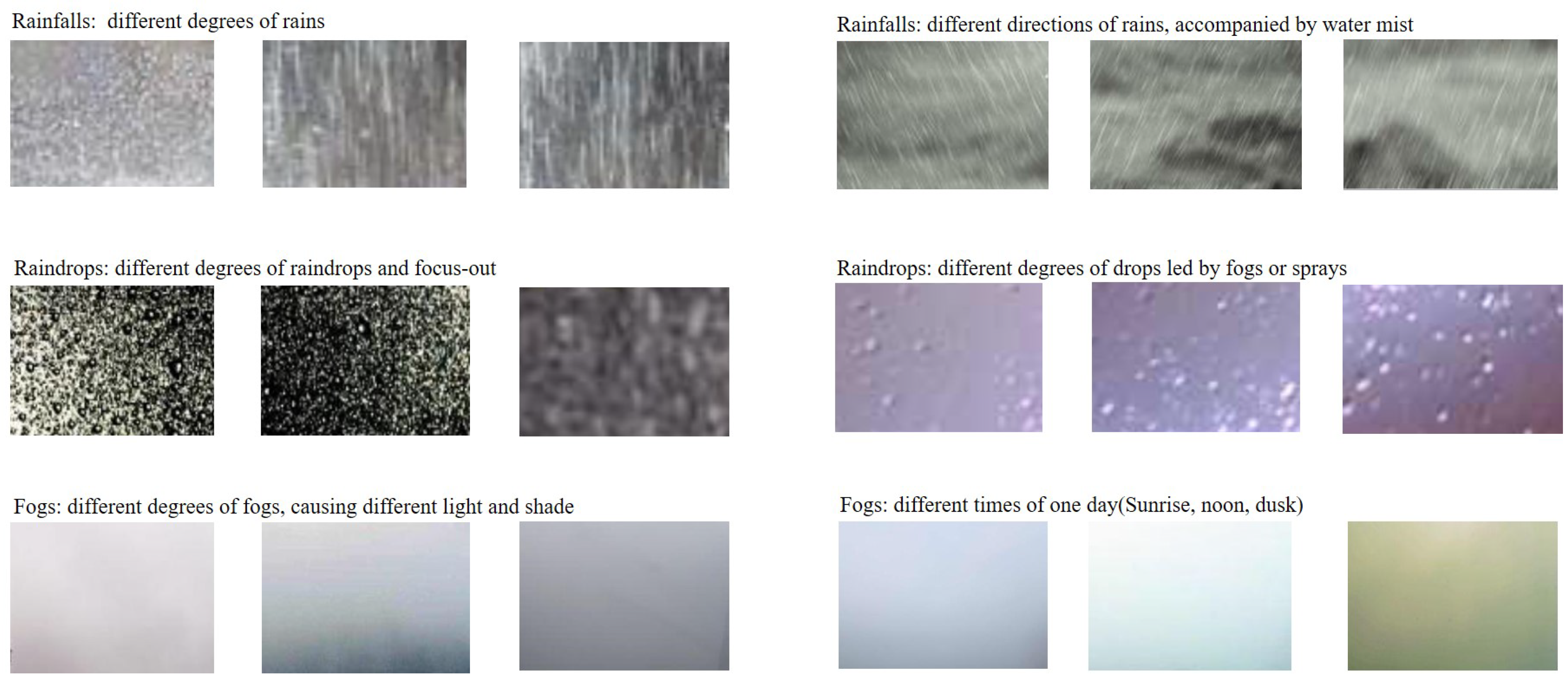
• We develop a rain–fog dataset containing 500 samples of pure rain–fog backgrounds. The pure images are collected from non-artificially synthesised scenes and the real world. This dataset is suitable for quantitatively validating ship detectors and testing the practical effects in marine environments.

2. Related Works

The ship detection of modern detectors has been introduced recently, while several conventional approaches have also been proposed for ship detection. According to the networks of conventional or modern detectors, ship detectors consist of traditional and modern ship detectors.

2.1. Traditional Ship Detectors

The traditional ship detectors, which focus on the background, mainly initialise the specified remote sensing or ship-borne video to establish the background model and utilise the difference to detect marine targets. Wang Mingfan et al. propose a Gaussian mixture model [27] to combine the contrast between local and global backgrounds, constraining the influence of phosphorescence under intense light. Xu Fang et al. establish a background model [28] based on the feature of remote sensing on the sea surface, which combines with the multiple modules to gain the target features according to the visual significance, and then unifies the thick and fine segmentation to detect the ship targets. Borghgraef et al. resort to the spatiotemporal correlation of dynamic background and introduce a surface floating-object algorithm [29] based on ViBe [30] and Behaviour Subtraction [31], which detects potentially dangerous objects by updating the background in a complex dynamic scene. Hu et al. propose a robust background-iterative algorithm [32], eliminating the influence of waves on the background to some extent, and a fast four-link module to accelerate the detection speed.

The traditional ship detectors, which focus on the foreground, build the ship detection model based on salient features or textures. According to the attention mechanism of human psychology, Itti et al. simulate the bottom-up visual selection processing of human beings and adopt Gaussian filtering and difference subtraction of feature expression [33] to obtain the detection model. Arshad et al. consider ship boundaries to localise ships by “thickening”, “expanding” and “bridging” operations [34], whose operations also combine background features to establish a real-time ship detector by morphological operations and differential framing methods. Fefilatyev et al. propose a sea-level monitoring algorithm [35] that can be installed on a fast-moving ship-borne platform according to the texture of the skyline, which effectively detects ships in a parallel perspective.

However, the target detectors designed on manual features have a large window calculation redundancy and instability, especially for various surrounding changes [10]. Unavoidably, while inheriting the advantages of interpretability, traditional ship detectors also gain the corresponding disadvantages of instability. Therefore, traditional ship detectors based on conventional detectors meet the plateau effect.

2.2. Modern Ship Detectors

Representative one-stage detectors, whose workflow unifies classifying processes and localizing regression into one regression, contain SSD [15], EfficientDet [21], YOLO series [16,17,18,19,20], etc. In particular, the YOLO series make non-negligible efforts to improve the better balance between inference and performance. YOLOv1 is an initial version and has a real-time speed, while the set anchors are initially fixed, leading to an unpractical and low accuracy [16]. To some extent, YOLOv2 improves the detection effects based on the Batch Normalization (BN) and adjustable anchors [17]. YOLOv3 adopts multiple output layers and DarkNet53 to unify the classification and location regression [18], achieving impressive improvement results. Recently, YOLOv4 and YOLOv5 are proposed and maintained based on the pre-version of the YOLO series [19,20]. YOLOv4 takes the “Bag of freebies” and “Bag of specials” to ensure a further impressive balance between inference and accuracy. Although YOLOv4 has a parallel performance or even outperforms the YOLOv5, YOLOv5s(the light model of YOLOv5) has fewer parameters and faster inference, which leaves more optimisation space for the post-adjustments, which becomes one basement of potential ship detectors.

Along with the mounting development of CNNs, modern ship detectors are gradually appearing, which utilise CNNs to automatically extract the target features and calculate the classification and position of the ship. Modern ship detectors are mainly built on two-stage and one-stage common detectors [16,17,18,19,36].

Modern ship detectors, built on two-stage common detectors, tend to achieve impressive performance without consideration of computational costs. R-DFPN [36] is proposed to improve the recall of ships in complex port scenarios by adding the rotation dimension based on the feature pyramid network. However, R-DFPN, belonging to two-stage networks with a complex network structure, and speeds less than 15 fps, makes it challenging to meet the real-time requirements. An autonomous ship-oriented method [37] is introduced by a novel hybrid algorithm that combines GAN and CNN. Nonetheless, the ship classes classified and inference are limited.

Modern ship detectors, constructed on one-stage common detectors, tend to better balance inference and accuracy compared with two-stage modern ship detectors. An enhanced ship detector [9] based on YOLOv3 detects multi-class ships with real-time inference speed, while the background and target collected are single to some extent. Although meeting the basic real-time speed(more than 25 fps), the inference speed hovers at approximately 30 fps, leaving less room for subsequent enhancements. Compared with the application of YOLOv3 in ship detection, YOLOv4 and YOLOv5 are platforms of potential ship detectors, owing to improved performance and relatively fast inference. Although YOLOv4 has a parallel performance or even outperforms the YOLOv5, YOLOv5s (the light model of YOLOv5) has fewer parameters and faster inference [20], which leaves more optimisation space for the post-adjustments. However, YOLOv5s lacks application and improvements corresponding to the marine surroundings. In addition, the lack of a ship dataset containing various scenes and a rain–fog dataset suitable for validating ship detectors is a non-negligible barrier.

2.3. Ship Datasets

In terms of the datasets used for ship detection, there is a serious lack of open datasets for intelligent maritime transport, compared with KITTI [22], Torontocity [23], and RobotCar [24] properly used for inland transportation. Public datasets, such as COCO [25] and VOC [26], have nearly 9000 ship samples, but the types of targets and ratios are single, and the scenes are simple. In addition, the corresponding public datasets tend to validate detectors in an ideal state, leading to the fact that the practical effects of ship detectors are rarely validated in actual application scenarios. The ship dataset [9] proposed by R.W Liu has relatively considerable targets compared with public datasets, while the most frequently detected backgrounds are the horizontal field of vision, lacking various angles, multi-dense states, multiple classes or target scenes, etc. In the absence of sufficient datasets related, it is difficult to give full play to the advantages of CNNs or the algorithms involved. Therefore, the establishment of ship and rain–fog datasets is essential in the field of ship detection.

3. Methodologies

Although YOLOv4-tiny (the tiny version of YOLOv4) decreases the training parameters, the average precision of YOLOV4-tiny is just 21.7% [20], far less than the YOLOv5s. YOLOv4 and YOLOv5 belong to the YOLO series and have fewer differences compared with the gap between YOLOv2 and YOLOv3. Furthermore, YOLOv5s better balance the performance and inference. Therefore, we decide to choose YOLOv5s as the optimization platform and construct our ship detector. This chapter proposes fast U-Net and remapping attention to improve the accuracy and robustness of the real-time ship detector under marine meteorological weather. The ship dataset is developed to increase the diversity of ship targets, and data augmentation of cross-background is mainly proposed for producing new detection backgrounds. The rain–fog dataset is introduced to validate the practical effects of detectors comprehensively.

3.1. Remapping Attention and Fast U-Net

Attention modules have been utilised to recommend CNN models “what” or “where” solutions, which are non-negligible methods to further prompt the accuracy of detectors. The popular attention modules, utilizing both space and channel features, contain CBAM [38] and Coordattention [39]. In particular Coordattention has been validated and approved recently by comparing various attention methods, such as SE attention [40], CBAM [38], and “X-Y” Attention [39]. However, the generalization ability is limited to some extent when validating situations are changing. Considering, especially, the improving of the robustness of YOLOv5s and retaining the balance of inference and accuracy in various marine weather conditions, remapping attention is proposed as shown in Figure 1. Remapping attention of space exploits the positional information by “Maxpool” and “AVGpool”, and then remaps the global space information to the local features by “softplus” activation. Remapping attention of the channel exploits the similar information remapped. Compared with the CBAM [38] and Coordattention [39], which both utilise the space and interchannel information, remapping attentions maintain local and global features of YOLOv5s (the light-version model of YOLOv5 [20]) by mapping the attention parameters to the probability adjustment. The probability adjustment based on local and global features is a reasonable assumption to boost the robustness in adverse weather conditions. Considering the cost of computation and GPU memory, the insertion position of remapping attention models is shown with $CBL+$ in Figure 2. The following experiments demonstrate that remapping attention obtains a relative peak compared to the CBAM [38] and Coordattention [39] and promotes robustness in fog–rain soaking conditions. The detailed workflow of remapping attention can be calculated as:

$$\left\{\begin{array}{cc}{C}_{atten}=F\left(\frac{K(APavg2d_{\left(1\right)}\left(\left(f\right)\right)+APmax2d_{\left(1\right)}\left(\left(f\right)\right))}{Su{m}_{dim=1}\left(K\left(\left(f\right)\right)\right)}\right)\hfill & \\ S_{atten}=F\left(\frac{K(MA{X}_{dim=1}\left(\left(f\right)\right)\cup AV{G}_{dim=1}\left(\left(f\right)\right))}{APavg2d\left(1\right)\left(\right(f\left)\right)}\right)\hfill & \\ Featur{e}_{pro}=S_{atten}\times C_{atten}\times \left(f\right)\hfill \end{array}\right.$$

(1)

where $C_{atten}$ and $S_{atten}$ are the remapping attention of space and interchannel, respectively. F is the activation function of “softplus”. K denotes the processing of kernels. $APavg2d_{\left(1\right)}$ and $APmax2d_{\left(1\right)}$ are the operations of “nn.AdaptiveAvgPool2d” and “nn.AdaptiveMaxPool2d” in the channel dimension. f and $Featur{e}_{pro}$ are the original features and enhanced features after the processing of $S_{atten}$ and $C_{atten}$. $MA{X}_{dim=1}$ and $AV{G}_{dim=1}$ are the “torch.mean” and “torch.max” functions in the dimension of the channel. “nn” and “torch”, imported from PyTorch, provide module tools for creating and training neural networks. During the utilisation of “nn.” and “torch.”, “Module” is an abstract concept representing either a layer in a neural network or a neural network with multiple layers.

The head of YOLOv5s is the “U” tube network, constructed to upsample the features by the two upsampling layers of “nn.Upsampling” operation, which is conducive to merging the semantic and detailed features. However, the “nn.Upsampling” operation is inefficient compared with indexing operations of tensors. The inference comparison of popular upsampling methods is shown in Figure 3. We utilise a laptop with RTX 2060 as the inference testing platform and collect the logs of inference speeds based on various testing batch sizes. The deconvolution spends the most time in the upsampling processing, which is the primary reason to abandon “Deconv” in the following experiments. “Pixelshuffle” is an efficient upsampling method, while the requirement of four times between channels of adjacent layers is incompatible with the heads of the network that is built. “nn.Upsampling” is a common upsampling method with the attribute of the broadest utilisation, which is the major reason to add “nn.Upsampling” to the following experiments. The fast U-Net is introduced by the indexing operations to further prompt the inference and robustness because of the appropriate decrease of parameters, whose structure is shown in the head of Figure 2. The reversing “Up” represents a fast U-Net which is most efficient compared with the others in Figure 2. The fast U-Net offered is shown in Figure 4. The tensors are indexed and sliced to double the resolutions by period distribution, while the channels are decreased which is conducive to indirectly compressing features and saving computing costs. Compared with the “nn.Pixelshuffle”, the $RandomCopy$ of Figure 5 ensures avoidance of not being divisible [41] and feature loss.

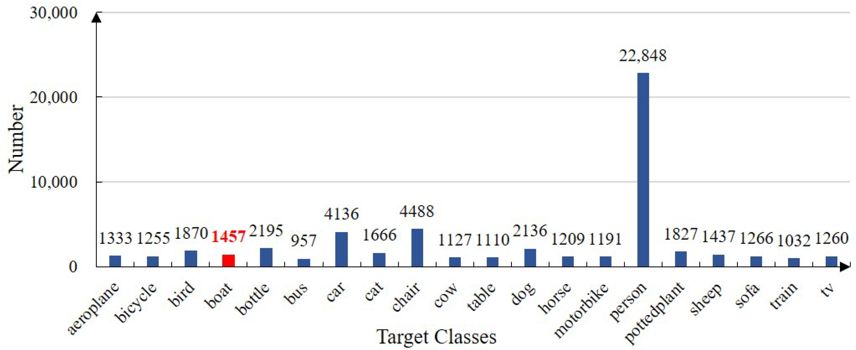
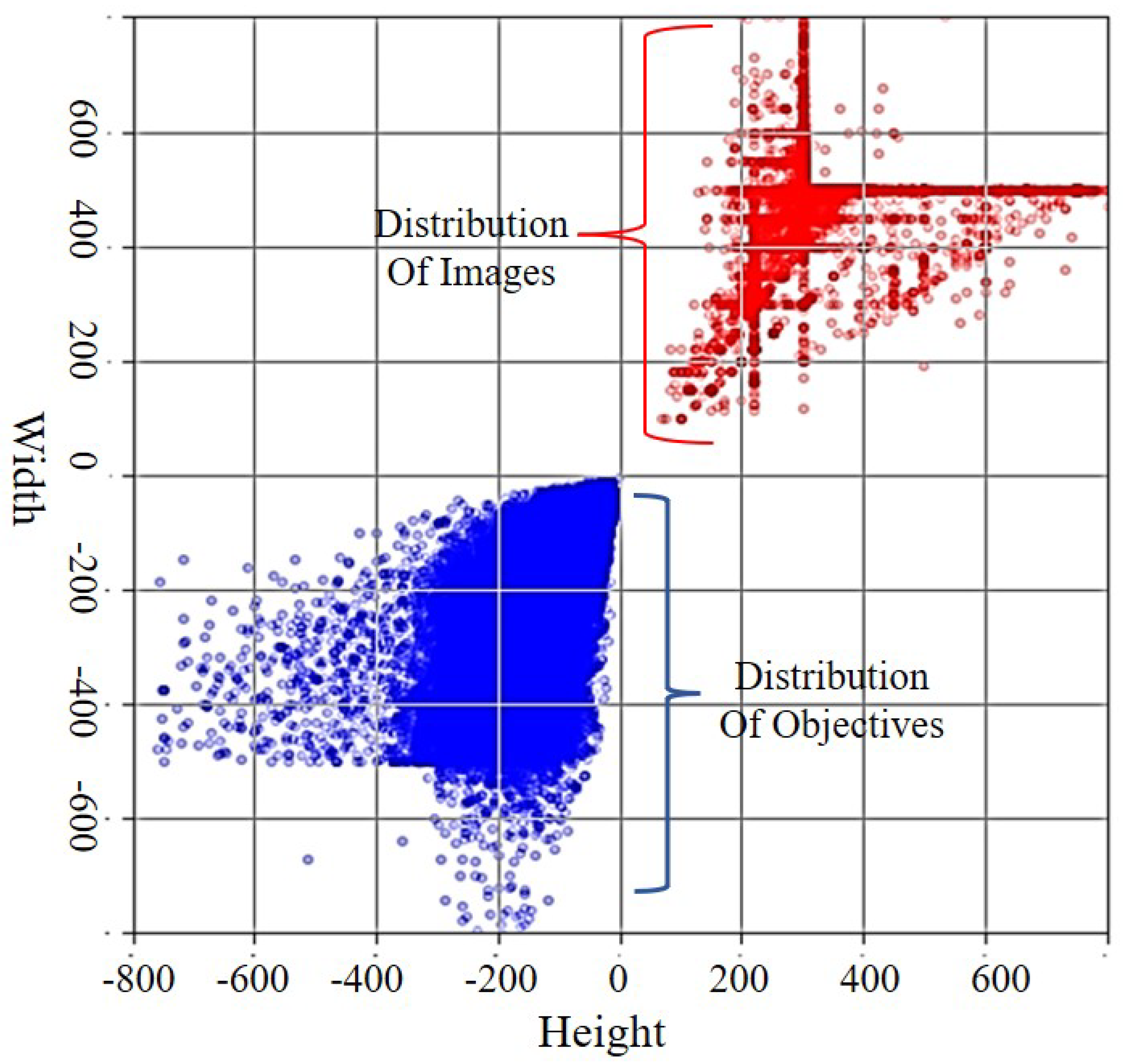
3.2. The Ship Dataset and Data Augmentation

VOC [26] and COCO [25] are public datasets for detection or segmentation. VOC contains about 20 classes of daily life, however all ships are labelled as “boat”. COCO is relatively more challenging. However, by converting and visualising COCO, we found that labels have more than one human error, a box which carelessly contains multiple targets and is resistant against training and testing to some extent when the number of samples is insufficient. The number of categories and labels of VOC used only for training are shown in Figure 5. The targets of the top three largest numbers are “person”, “chair”, and “car”, respectively. There are more than 20,000 samples of “person”, while the amount of “boat” is just 1457. The size distribution of the “boat” in VOC is shown in Figure 6. The absolute values of the horizontal and vertical axes are the width and height of the images and targets. Red and blue dots represent an image and a target, respectively. The distribution in the upper right corner shows the size distribution of images, those in the lower-left corner show the size distribution of the “boat”, and the colour depth indicates the degree of concentration. The length or width of the images is mainly constrained to 500, which is evenly distributed in a line, while the corresponding “boat” is excessively concentrated in the area of “200 × 200”. Although VOC meets the requirements of ship detection to some extent, the distribution is single with only 1457 targets. The target distribution is too concentrated in one location, lacking diversity distribution. If 1457 targets and labels are used as the training dataset of ship detectors, the training process is prone to overfitting. Therefore, it is necessary to establish a dataset containing substantial ship targets and ample classes, which brings into full play the advantages of CNN.

Due to the requirement to visualise producing the ship dataset, this paper further develops the datasets [42] based on the format of VOC [26]. The ship dataset proposed contains 21,000 samples, subdivided into eight classes and one unidentified class. Eight ship classes are eight specific categories which can be distinguished when we label the targets, while unidentified ships are categorised into a class in which the specific class is indistinguishable and we label unidentified ships with “ship”. Our ship dataset has two components, “VOC-ship” and “VOC-ship-test”, utilised for the training and testing, respectively. Both VOC-ship and VOC-ship-test consider the weather factors, such as detection angles, light, and dense occlusion. The specific classes and numbers of our ship dataset are shown in Figure 7. The ship classes contain “engineering_ship, freighter, passenger_ship, public_service_vessel, sailboat, speedboat, submarine, warship,” and the numbers of training and testing targets are “1179, 2604, 802, 2311, 2749, 3145, 2625, 1163” and “515, 638, 241, 499, 650, 782, 685, 320”, respectively. The steps to make the ship datasets are as follows: (1) we use cameras to capture multiple scenes while utilising Google Chrome and a plug-in to crawl ship pictures. (2) We delete pictures with low quality through manual screening, classify ships filtered, and name pictures in batches with Arabic numerals. (3) We utilise the “labelImg” downloaded from GitHub to make labels, and label files are XML format which is conducive for visualisation. The code of “labelImg” is https://github.com/tzutalin/labelImg (accessed on 26 July 2022).

The target distribution of our ship dataset is shown in Figure 8. The denotation of light-red and light-blue dots is the same as the presentations in Figure 6. The images of our dataset are concentrated in the area near “$500\times 500$”. The corresponding targets are focused on the room with a length or width of “0–500”. In addition, there are also enough middle or large targets in our ship dataset, shown in the area of “500–800”, which meets the requirements of medium-range detection utilising common cameras. Compared with Figure 6, the targets of our ship dataset are more evenly distributed in the range of “$500\times 500$” while increasing the number and aspect ratios of targets. Comprehensively, the ship dataset proposed has the ratio diversity of targets and potentially exploits the advantages of visible-light cameras to form a match with the remote detection technology. Part samples of our ship datasets are shown in Figure 9, which also demonstrates the factors considered to build the ship dataset, containing multiple detection angles. Different detection angles show that the detectors, trained by VOC-ship, can be used in static shore-based detection scenes, as well as shipborne or airborne detection scenes.

The data augmentations of YOLOv5 are practical to enhance the value of samples, while the stability of ship navigation is relatively complicated, especially in this case that the shipboard camera detects other ships under the influence of rains and waves, leading to a complexing background. To increase the diversity of detecting surroundings, data augmentation of the cross-background is introduced to increase the diversity of detecting backgrounds, as shown in Figure 10. A larger merged image contains 4 middle merged images. The copied targets have a location in the new background, which releases the relative lack of background diversity in ship datasets and enhances the utilisation of the remaining grey area.

3.3. The Rain-Fog Dataset

VOC [26] and COCO [25] are public datasets for the detection and segmentation of common targets. However, the corresponding testing datasets tend to validate detectors in an ideal state, leading to the fact that the robustness of ship detectors is hardly validated in an adverse environment. Therefore, collecting a rain–fog dataset suitable for the marine environment is necessary to validate the practicability of ship detectors. Considering adverse impacts from rainy or foggy weather, the SPA [43], Rain100H [44], and Rain1400 [45] have been offered to minimize the influence of bad weather. However, the rain datasets above are mainly utilized for the rain removal of inland environments. In addition, the public rain datasets have a few pure images only having little rain or drops, which hardly meet the requirements of soaking ship images. Most backgrounds of rain datasets are cut or synthetically made from entire images, and the backgrounds have buildings and streets, hardly representing the marine surroundings, such as the rain–fog crossing scenes and raindrops created by rain or waves. Our rain–fog dataset contains 550 images with pure weather backgrounds, which consist of pure rainy or foggy scenes, rain–fog crossing scenes, and raindrops wetting lenses. The steps for collecting pure rain–fog images are similar to the ship dataset, except for the labelling processing. The images of the rain–fog dataset are entire images collected from the real world without artificial data interference. To enhance the value of the rain–fog dataset, we can randomly choose rain–fog images to paste or soak the testing images in staggered repetition. Part of the images soaked by different degrees are shown in Figure 11, and classic scenes of the rain–fog dataset are shown in Figure 12. The soaking operation is based on the Python Imaging Library (PIL), and the different soaking degrees are set from 0.4 to 0.8. The adverse marine scenes are more complicated than the major scenes of public rain–fog datasets, which are suitable for the rain removal task of the inland environment. Our rain–fog dataset is built by considering various adverse weather conditions and scenes, which appropriately simulate the marine environment. Compared to rain datasets containing buildings and streets, our rain–fog dataset is more suitable for quantitatively testing the practical effects of ship detectors based on deep learning.

4. Experiments and Results

4.1. Experimental Setting

4.1.1. Experimental Conditions

The experimental software contains Ubuntu 16.04.4, PyTorch 1.7, and CUDA10.2. TITAN V and RTX 2080ti are GPUs utilised. If not specifically mentioned, TITAN V is the default device.

4.1.2. Datasets

The datasets, utilised in our manuscript, contain COCO [25], VOC-ship, VOC-ship-test, and rain–fog datasets. COCO [25] is a public dataset containing training and testing components, which can be used to, respectively, train and test the common detectors. Correspondingly, the ship dataset proposed consists of VOC-ship and VOC-ship-test. VOC-ship is utilised for the training ship detectors that participated. VOC-ship and VOC-ship-test are the ship datasets we proposed. VOC-ship is used to train ship detectors and VOC-ship-test is utilised to test ship detectors. The training samples of our ship dataset are shown in Figure A1. The rain–fog dataset proposed is a pure rain–fog image collection which can validate the practical generalisation ability of ship detectors.

4.1.3. Parameter Setting

With regard to the FRSD training in COCO [25], the detailed settings are as follows: Epochs: 300; Batch Size: 32; Image Size: $640\times 640$; Initial Learning Rate: $1\times$${10}^{-3}$; Optimizer: $Adam$; Adam Beta1: ($0.3$$0.6$$0.98$); and Data Augmentation: Mosaic augmentation. With regard to the FRSD training in VOC-ship, the detailed settings are following: Epochs: 300; Batch Size: 64; Image Size: $640\times 640$; Initial Learning Rate: $e^{-2}$; Optimizer: $Adam$; Adam Beta1: ($0.3$ $0.6$ $0.98$); and Data Augmentation: Data Augmentation of Cross-background (at the time of mention). Detectors who participated take their own published parameters. Concerning the testing in the VOC-ship-test, the $FPS$ is contained with a batch size of 1, and inference augmentation is unset. Rain–fog dataset randomly soaks the testing images to the degree of “0, $0.4$, $0.5$, $0.6$, $0.7$, $0.8$”. The loss function used in the training step of FRSD relevant is as follows:

$$\left\{\begin{array}{cc}{L}_{class}=-\sum _{n=i}^N(x_i^{*}log\left(\frac{1}{1+e^{-x_i}}\right)+(1-x_i^{*})log\left(\frac{e^{-x_i}}{1+e^{-x_i}}\right))\hfill & \\ L_{location}=1-(IOU-{\left(\frac{D_{angles}}{D_{centers}}\right)}^2-\frac{{\alpha }^2}{1-IOU+\alpha })\hfill & \\ L_{confi}=(1-i{f}_{gt})+i{f}_{gt}\ast IO{U}_{score}\hfill & \\ Tota{l}_{loss}=L_{class}+L_{location}+L_{confi}\hfill \end{array}\right.$$

(2)

where $x_i^{*}$ and $x_i$ are the probability of the category predicted and Ground Truth, respectively. $D_{angles}$/$D_{centers}$ is the contrast value of $Distance$ of opposite angles and centers. $\alpha$ is a parameter that measures the consistency of aspect ratio. $IOU$ is the union ratio of the prediction box to the $GT$ box (Ground Truth). $i{f}_{gt}$ denotes that there is or is not a target in the noticing area. The square root of $\alpha$ is set as 2/$\pi \times \left(arctan\right(W_{gt}$/$H_{gt})-arctan(W_{pred}$/$H_{pred}\left)\right)$.

4.1.4. Data Augmentation

The data augmentation of the cross-background is controlled by $Thresh$, $Prob$, $Copy\_times$, and $Epochs$, which are set to $50\times 50$, $0.5$, 3, and 30. $Thresh$ is the threshold of the object copied whose $H\times W<thresh$, $Prob$ is the probability of copy occurring, $Copy\_times$ is the times to be copied, and $Epochs$ represents that the data augmentation proposed is efficient until the $Epochs$ set.

4.1.5. Metrics

The metrics utilised to validate the performance of detectors contain average precision (AP) and other metrics based on AP. Frames per second (FPS) is the popular measurement to represent the running or processing time. The higher the FPS value, the better the real-time performance of the algorithm. The detailed concepts are the following:

$$AP={\int }_0^1{p}_{smooth}\left(r\right)dr\iff \sum _{r=0}^1\left(r_{n+1}-r_n\right)\underset{\tilde{r}:\tilde{r}\ge r_{n+1}}{max}p\left(\tilde{r}\right)$$

(3)

where $p_{smooth}\left(r\right)$ and $p\left(\tilde{r}\right)$ are the max value of precision recall(PR) after smoothing the curve of PR. $\tilde{r}:\tilde{r}\ge r_{n+1}$ represent the split points of precision recall.

$A{P}_{0.5:0.95}$: The threshold of intersection over union (IOU) is adjusted from a fixed 0.5 to calculate the multi-AP values at intervals of 0.5 to 0.95, and the average of all results is taken as $A{P}_{0.5:0.95}$.

$A{P}_{50}$ and $A{P}_{75}$: The AP is gained when the IOU is set to 0.5 and 0.75, respectively.

$A{P}_S$, $A{P}_M$, and $A{P}_L$: The AP is gained when pixel areas of targets set are $0:{32}^2$, ${32}^2:{96}^2$, and ${96}^2:end$, respectively.

$FPS$: Frames per second(FPS) denotes the number of images processed per second and directly the real-time effect of algorithms.

4.2. Results

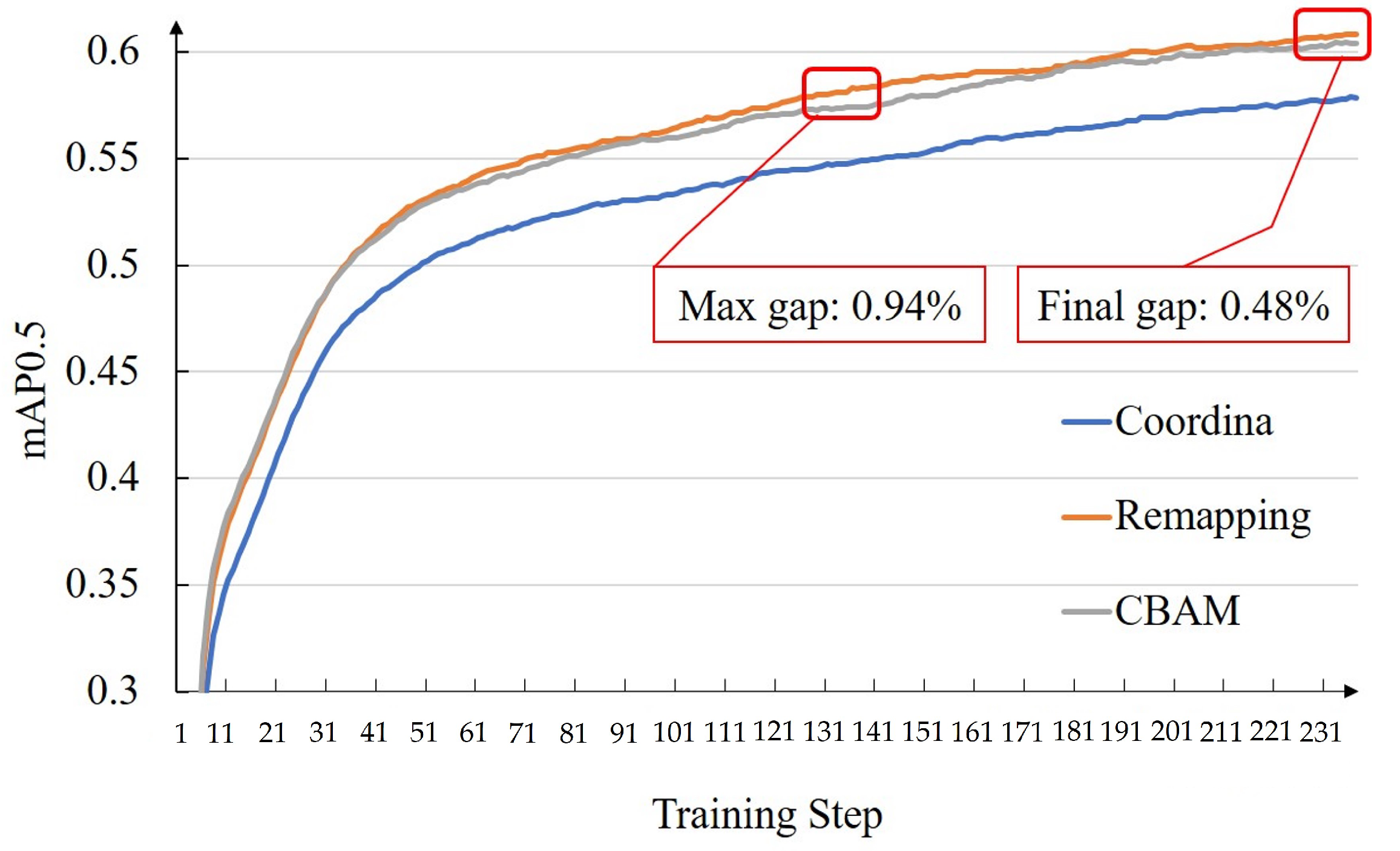
4.2.1. Influence of the Remapping and Fast U-Net

Comparing YOLOv5s_ReMap_FastUnet (another denotation of FRSD) with other public detectors in COCO [25] is the first step to constructing robust ship detectors, which is necessary to validate the remapping attention and fast U-Net in the public dataset. The comparison of popular detectors in the public dataset is shown in

Table 1. Comparison of detectors in COCO (devtest2019) [25]. To distinguish algorithms, FRSD is denoted by “YOLOv5s_ReMap_FastUnet”. The batch sizes of all detectors are set to 1 in the testing stage. To display the inference boosting of fast U-Net, the batch sizes of YOLOv5s_ReMap_Unet and YOLOv5s_ReMap_FastUnet are set to 1 and 10, respectively, and the values before and after “/” correspondingly represent the inference speed.

Detectors	Backbone	ImgSize	FPS	${\mathit{AP}}_{0.5:0.95}$	${\mathit{AP}}_{50}$	${\mathit{AP}}_{75}$	${\mathit{AP}}_{\mathit{S}}$	${\mathit{AP}}_{\mathit{M}}$	${\mathit{AP}}_{\mathit{L}}$
SSD300 [15]	VGG16	300	43.2	0.251	0.431	0.258	0.066	0.259	0.414
Faster RCNN [12]	ResNet-50	1000	9.4	0.398	0.592	0.435	0.218	0.426	0.507
RetinaNet [47]	ResNet-101	800	5.1	0.378	0.575	0.408	0.202	0.411	0.492
CenterNet [48]	Hourglass-104	512	4.2	0.449	0.624	0.481	0.256	0.474	0.574
EfficientDet [21]	EfficientDet-B0	512	62.3	0.338	0.525	0.358	0.12	0.383	0.512
YOLOv4s [19]	CSPDarknet-53	416	38.0	0.412	0.628	0.443	0.204	0.444	0.56
YOLOv5s [20]	CSPDarknet-53	640	69.9	0.369	0.561	0.4	0.196	0.413	0.457
YOLOv5s_Unet	CSPDarknet-53	640	59.0	0.393	0.582	0.431	0.23	0.432	0.466
YOLOv5s_Coord_Unet	CSPDarknet-53	640	48.7	0.396	0.587	0.433	0.232	0.436	0.468
YOLOv5s_CBAM_Unet	CSPDarknet-53	640	45.87	0.424	0.615	0.465	0.254	0.462	0.512
YOLOv5s_ReMap_Unet	CSPDarknet-53	640	43.5/263.2	0.425	0.617	0.465	0.251	0.463	0.513
YOLOv5s_ReMap_FastUnet	CSPDarknet-53	640	40.3/278.4	0.425	0.617	0.465	0.251	0.463	0.513

. YOLOv5s_Unet is the detector utilizing three “nn.Upsampling” layers in the head network of YOLOv5s. YOLOv5s_CBAM_Unet, YOLOv5s_Coord_Unet, and YOLOv5s_ReMap_Unet are the detectors using the CBAM [38], Coord [39], and remapping methods, respectively. CBAM and Coord are inserted into the backbone, whose position is the same as the remapping attention in the FRSD. Compared with the results of YOLOv5s_Unet and detectors promoted by three attention insertions, attention methods reliably prompt the accuracy. The $A{P}_{50}$ of YOLOv5s_ReMap_Unet has increased by 3.5%, 3%, and 0.2%, respectively, compared with YOLOv5s_Unet, YOLOv5s_Coord_Unet, and YOLOv5s_CBAM_Unet, demonstrating the rationality of the remapping method. Especially, the most gap of the $A{P}_{50}$ between YOLOv5s_ReMap_Unet and YOLOv5s_CBAM_Unet reaches approximately 1%, as shown in Figure 13, indicating that the remapping attention proposed has the potential advantage of promoting the robustness in rainy and foggy weather, because of the relatively high performance in the case of undertraining conditions. YOLOv5s_ReMap_FastUnet maintains almost the same speed when the batch size is set to 1 compared with YOLOv5s_ReMap_Unet. Owing to the compression of the channel by the fast U-net, as shown in Figure 4, the inference speed increases by 15 fps to 278.4 fps when multiple batches are taken in the testing stage, which is suitable for the multi-task model and suggests the rationality of the fast U-Net. YOLOv5s_ReMap_FastUnet has a slightly lower speed than YOLOv5s_ReMap_Unet when the testing batch is set to 1, which the seemingly weird result is led by the preprepared production of double-size features. The advantages of fast U-Net are more visible when the testing batch size is set to multiple batches. Although the remapping attention and fast U-Net have an unimpressive influence on YOLOv5s_ReMap_FastUnet when adopting the testing images of COCO, the practical effect is visible in the rain–fog soaking situation, as shown in

Table 2. Comparison of ship detectors in the VOC-ship-test. FRSD_ship_dataaug is the final model which utilizes the data augmentation of the cross-background. Soaking 0.0−0.8 denote the mean average precision under the different levels of influence corresponding to the rain–fog dataset. FRSD_CBAM_FU and FRSD_FU are the ship detectors utilizing CBAM and remapping methods proposed in the backbone, respectively. “U” and “FU” denote the upsampling methods of “nn.Upsampling/nn.interpolate” and fast U-Net in heads, respectively. The positive impacts of fast U-Net and remapping attentions proposed are more visible under the most severe rain–fog wetting conditions (Soaking 0.8).

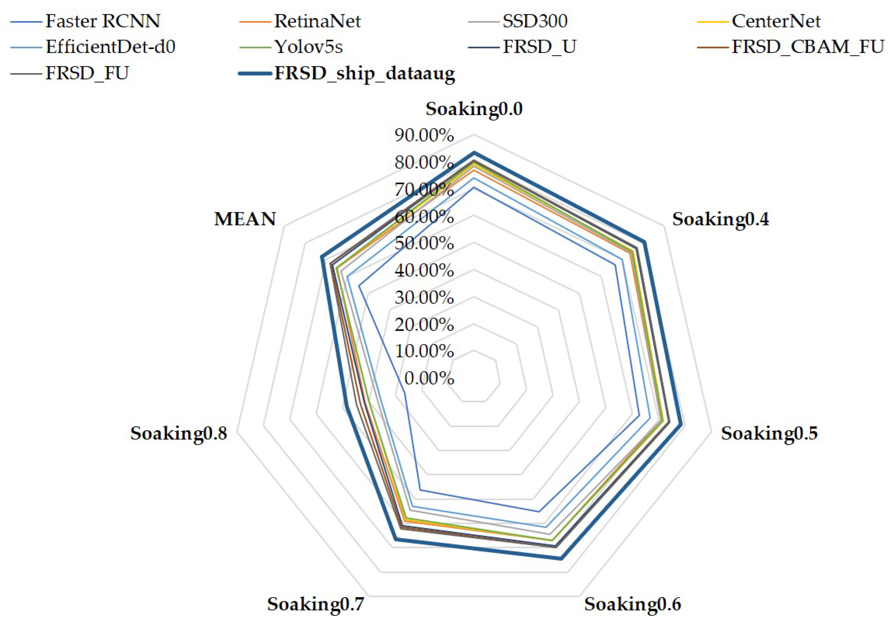
Detectors	Imgsize	Soaking 0.0	Soaking 0.4	Soaking 0.5	Soaking 0.6	Soaking 0.7	Soaking 0.8	MEAN	DEV	FPS
Faster RCNN [12]	800	70.59%	66.75%	62.65%	55.13%	46.16%	26.27%	54.592%	16.38%	25.10
RetinaNet [47]	600	76.90%	73.92%	70.98%	66.92%	58.98%	41.49%	64.865%	13.03%	34.61
SSD300 [15]	300	78.30%	74.40%	70.90%	64.50%	54.40%	36.70%	63.20%	15.45%	66.02
CenterNet [48]	512	78.70%	75.20%	71.90%	66.90%	58.300%	39.80%	65.13%	14.30%	42.30
EfficientDetd0 [21]	512	74.00%	70.10%	66.80%	61.50%	52.80%	35.50%	60.12%	14.13%	36.40
YOLOV4_ship [19]	416	74.26%	69.19%	65.81%	61.17%	52.22%	36.37%	59.87%	13.72%	34.20
YOLOV5s_ship [20]	640	78.79%	74.90%	71.60%	66.90%	57.80%	40.00%	65.16%	14.41%	68.01
FRSD_U	640	80.10%	76.70%	73.90%	69.10%	60.90%	41.80%	67.08%	14.07%	43.61
FRSD_CBAM_FU	640	80.19%	76.90%	74.10%	69.78%	61.60%	43.30%	67.65%	13.55%	43.31
FRSD_FU	640	80.39%	76.90%	74.20%	69.80%	62.22%	44.50%	68.01%	13.12%	42.56
FRSD_ship_dataaug	640	83.15%	80.70%	78.40%	74.50%	66.60%	48.40%	71.958%	12.91%	42.56

. The immediate influence of the fast U-Net on features is shown in Figure 14. Features of fast U-Net have more visible sparsity compared with the upsampling method of “nn.Upsampling”, which suggests why fast U-Net is evident when the channels are indirectly compressed.

4.2.2. The Comparison of Ship Detectors

The robustness of ship detectors in the VOC-ship-test is shown in Table 2, in which all ship detectors are validated on the same software and hardware, and the GPU used is 2080ti. Soaking 0.4 to 0.8 represent the mean average precision of ship detectors under different rain–fog soaking, in which the higher the number at the end, the more intrusive soaking degree. Although a better performance without considering the inference speed is achieved compared with YOLOv5s, YOLOv4 has a unimpressive practical detection results in multiple rain–fog scenes. YOLOV5s_ship and YOLOv5s_ReMap_ship are the ship detectors directly based on YOLOV5s and YOLOv5s_ReMap_Unet, and YOLOv5s_ReMap_Unet is the detector adopting only the remapping method in the YOLOV5s. FRSD_CBAM_FU and FRSD_FU are the ship detectors utilizing CBAM and remapping methods in the backbone, respectively, and “FU” denotes the fast U-Net in the head network. FRSD_FU maintains a real-time inference speed, reaching 42.56 fps, which meets the real-time ship detection. After the prompts of data augmentation proposed, FRSD_ship_dataaug have an impressive performance. The mean average precision of FRSD_ship_dataaug reaches the best under different soaking levels, reaching 83.30%, 80.50%, 78.00%, 74.40%, 67.40%, and 51.10%, respectively. Compared with FRSD_U, FRSD_FU achieves a lower deviation and better accuracy, suggesting that the fast U-Net also prompts robustness in the fog–rain conditions except for the inference speed accelerating. Meanwhile, FRSD_FU obtains better accuracy than FRSD_CBAM_FU, suggesting that remapping attention has the advantage of promoting robustness in rain–fog weather, and the probability adjustment based on the remapping attention proposed is a reasonable assumption to boost the robustness in adverse weather. FRSD_ship_dataaug has the best accuracy and lowest deviation, demonstrating that the data augmentation of the cross-background is effective. A more impressive comparison of ship detectors’ robustness is shown in Figure 15. The average precision of specific ship classes is shown in

Table 3. Comparison of ship detectors for specific ship detection. FRSD_ship_dataaug is the final model which utilizes the data augmentation of the cross-background during the training period. “ship” is categorised into a class in which the location is detected while the specific class is indistinguishable.

Detectors	Imgsize	Engi_ship	Freighter	Passe_ship	Public_ser	Sailboat	Speedboat	Submarine	Warship	Ship
Faster RCNN [12]	800	70.70%	85.55%	59.68%	86.36%	79.67%	85.81%	87.78%	65.08%	14.72%
RetinaNet [47]	600	81.58%	93.31%	69.60%	90.35%	86.35%	91.79%	87.58%	77.72%	13.80%
SSD300 [15]	300	84.37%	88.77%	78.08%	88.61%	82.22%	87.31%	90.21%	85.10%	20.47%
CenterNet [48]	512	77.60%	91.70%	75.00%	92.50%	85.70%	90.50%	92.50%	81.90%	20.05%
EfficientDetd0 [21]	512	74.10%	90.40%	66.40%	89.10%	87.30%	89.80%	88.10%	72.70%	11.30%
YOLOV5s_ship [20]	640	71.10%	92.00%	72.20%	91.79%	88.10%	91.40%	94.20%	84.40%	23.90%
FRSD_ship_dataaug	640	84.70%	94.20%	80.60%	93.70%	89.20%	93.90%	95.01%	85.80%	26.90%

. The “ship” class represents the ship target is detected while the specific class is indistinguishable. The detection results of FRSD are shown in Figure 16, Figure 17 and Figure 18.

5. Discussion

Ship detectors are mainly dependent on radars or remote sensing satellites, partially, but significantly, because of the relatively complex hydrology and the advantages of remote monitoring. Advanced radars detect not just ships with intense precision and even real-time speed, while satellites obtain extraordinary resolution images in the sky, containing ample information. Nevertheless, it is not economical and is wasteful to utilize remote monitoring systems in ship detection over short or medium ranges. Advanced radars are impressively money-consuming even after adopting products to reduce costs, without consideration of follow-up tedious maintenance, satellites are scarce in terms of expensive launching costs and limited service life. Compared with the detection technologies above, although ship detection utilizing visible-light cameras is susceptible to rain and fog, the observation distance reaches more than 10 km under ideal weather conditions. More importantly, the information obtained by visible-light sensors is more abundant.

Therefore, this paper considers that ship detection based on standard cameras should form a low and high collocation with radars or other technologies suitable for far-sightedness. We propose a ship detector based on fast U-Net and remapping attention (FRSD). With the datasets proposed and the novel methods, FRSD performs relatively robustly and detects 9 classes with an mAP of more than 83%, and the practical robustness is fully validated, reaching a state-of-the-art level. The practical performance in rain-fog conditions is further displayed in Figure A2. Therefore, the FRSD proposed has an impressive capacity to build a low and high collocation with radars or other technologies suitable for far-sightedness. We believe that the cooperation of FRSD and remote detection skills should improve the management of maritime security and transport.

Although our ship detector has impressive performance in the related field, this paper also has limitations. The rain–fog dataset proposed is only suitable for validating the practical effects of ship detectors and hardly meets the requirements of model training. Although the ship dataset proposed has considerable samples, the original fog–rain scenes of the ship dataset are fewer compared with the practical marine environments. The ship detector proposed has the initial anti-adverse weather ability. However, the mean average precision decreases impressively in full rainy or fog weather. Suppose we enable the anti-adverse weather ability to the detection algorithm. In that case, the real-time effect of FRSD template hardly meets post-improvement, which easily leads to a visible decrease in inference speed. Overcoming the shortcomings is our next direction, we will build a ship detector of anti-adverse weather by proposing novel methods.

6. Conclusions

The remapping attention method and fast U-Net are proposed to gain a real-time ship detector suitable for various ocean weather conditions. Remapping attention combines the local and global features that are relatively compatible with YOLOv5s. Fast U-Net compresses the parameters by the index operation, accelerating the inference speed when multiple batches are set and increasing stability in various weather conditions. The ship dataset is offered to alleviate the lack of multiple ship datasets, and the data augmentation of the cross-background is proposed to increase the value of the ship dataset. The rain–fog dataset is introduced to quantitatively validate the ship detectors. Experiments demonstrate that FRSD detects 9 classes with an mAP of more than 83%, and the practical robustness is fully validated by a quantitatively soaking method, reaching relevant state-of-the-art ship detectors.

References

- Xiao, R.; Jianga, S.; Zhongb, J. Status and Development Trend of Active Sub-arrays Structure Design in Active Phased Array Antenna. IOP Conf. Ser. Mater. Sci. Eng. 2020, 914, 012038. [Google Scholar] [CrossRef]
- Wang, X.; Li, G.; Zhang, X.P.; He, Y. A Fast CFAR Algorithm Based on Density-Censoring Operation for Ship Detection in SAR Images. IEEE Signal Process. Lett. 2021, 28, 1085–1089. [Google Scholar] [CrossRef]
- Gao, F.; He, Y.; Wang, J.; Hussain, A.; Zhou, H. Anchor-free convolutional network with dense attention feature aggregation for ship detection in SAR images. Remote Sens. 2020, 12, 2619. [Google Scholar] [CrossRef]
- Cui, Z.; Li, Q.; Cao, Z.; Liu, N. Dense attention pyramid networks for multi-scale ship detection in SAR images. IEEE Trans. Geosci. Remote Sens. 2019, 57, 8983–8997. [Google Scholar] [CrossRef]
- Caon, M.; Ros, P.M.; Martina, M.; Bianchi, T.; Magli, E.; Membibre, F.; Ramos, A.; Latorre, A.; Kerr, M.; Wiehle, S.; et al. Very low latency architecture for earth observation satellite onboard data handling, compression, and encryption. In Proceedings of the 2021 IEEE International Geoscience and Remote Sensing Symposium IGARSS, Brussels, Belgium, 11–16 July 2021; pp. 7791–7794. [Google Scholar]
- Solari, L.; Del Soldato, M.; Raspini, F.; Barra, A.; Bianchini, S.; Confuorto, P.; Casagli, N.; Crosetto, M. Review of satellite interferometry for landslide detection in Italy. Remote Sens. 2020, 12, 1351. [Google Scholar] [CrossRef]
- Krišto, M.; Ivasic-Kos, M.; Pobar, M. Thermal object detection in difficult weather conditions using YOLO. IEEE Access 2020, 8, 125459–125476. [Google Scholar] [CrossRef]
- Wang, N.; Li, B.; Wei, X.; Wang, Y.; Yan, H. Ship Detection in Spaceborne Infrared Image Based on Lightweight CNN and Multisource Feature Cascade Decision. IEEE Trans. Geosci. Remote Sens. 2020, 59, 4324–4339. [Google Scholar] [CrossRef]
- Liu, R.W.; Yuan, W.; Chen, X.; Lu, Y. An enhanced CNN-enabled learning method for promoting ship detection in maritime surveillance system. Ocean Eng. 2021, 235, 109435. [Google Scholar] [CrossRef]
- Pang, G.; Shen, C.; Cao, L.; Hengel, A.V.D. Deep learning for anomaly detection: A review. ACM Comput. Surv. (CSUR) 2021, 54, 1–38. [Google Scholar] [CrossRef]
- Girshick, R. Fast R-CNN. In Proceedings of the IEEE International Conference on Computer Vision, Santiago, Chile, 11–18 December 2015; pp. 1440–1448. [Google Scholar] [CrossRef]
- Ren, S.; He, K.; Girshick, R.; Sun, J. Faster R-CNN: Towards real-time object detection with region proposal networks. Adv. Neural Inf. Process. Syst. 2015, 28, 91–99. [Google Scholar] [CrossRef] [PubMed]
- Girshick, R.; Donahue, J.; Darrell, T.; Malik, J. Rich feature hierarchies for accurate object detection and semantic segmentation. In Proceedings of the 27th IEEE Conference on Computer Vision and Pattern Recognition (CVPR), Columbus, OH, USA, 24–27 June 2014; pp. 580–587. [Google Scholar] [CrossRef]
- Yang, Z.; Liu, S.H.; Hu, H.; Wang, L.; Lin, S. RepPoints: Point Set Representation for Object Detection. In Proceedings of the IEEE/CVF International Conference on Computer Vision (ICCV), Seoul, Korea, 27–28 October 2019; pp. 9656–9665. [Google Scholar] [CrossRef]
- Liu, W.; Anguelov, D.; Erhan, D.; Szegedy, C.; Reed, S.; Fu, C.Y.; Berg, A.C. SSD: Single Shot MultiBox Detector. In Proceedings of the 14th European Conference on Computer Vision (ECCV), Amsterdam, The Netherlands, 11–14 October 2016; Volume 9905, pp. 21–37. [Google Scholar] [CrossRef]
- Redmon, J.; Divvala, S.; Girshick, R.; Farhadi, A. You Only Look Once: Unified, Real-Time Object Detection. In Proceedings of the 2016 IEEE Conference on Computer Vision and Pattern Recognition (CVPR), Las Vegas, NV, USA, 27–30 June 2016; pp. 779–788. [Google Scholar] [CrossRef]
- Redmon, J.; Farhadi, A. YOLO9000: Better, Faster, Stronger. In Proceedings of the 30th IEEE/CVF Conference on Computer Vision and Pattern Recognition (CVPR), Honolulu, HI, USA, 21–26 July 2017; pp. 6517–6525. [Google Scholar] [CrossRef]
- Redmon, J.; Farhadi, A. Yolov3: An incremental improvement. arXiv 2018, arXiv:1804.02767. [Google Scholar]
- Wang, C.Y.; Bochkovskiy, A.; Liao, H.Y.M. Scaled-YOLOv4: Scaling Cross Stage Partial Network. In Proceedings of the IEEE/CVF Conference on Computer Vision and Pattern Recognition (CVPR), Nashville, TN, USA, 20–25 June 2021; pp. 13024–13033. [Google Scholar] [CrossRef]
- Ge, Z.; Liu, S.; Wang, F.; Li, Z.; Sun, J. Yolox: Exceeding yolo series in 2021. arXiv 2021, arXiv:2107.08430. [Google Scholar]
- Naddaf-Sh, S.; Naddaf-Sh, M.M.; Kashani, A.R.; Zargarzadeh, H. An Efficient and Scalable Deep Learning Approach for Road Damage Detection. In Proceedings of the 8th IEEE International Conference on Big Data (Big Data), Atlanta, GA, USA, 10–13 December 2020; pp. 5602–5608. [Google Scholar] [CrossRef]
- Geiger, A.; Lenz, P.; Urtasun, R. Are we ready for Autonomous Driving? The KITTI Vision Benchmark Suite. In Proceedings of the IEEE Conference on Computer Vision and Pattern Recognition (CVPR), Providence, RI, USA, 16–21 June 2012; pp. 3354–3361. [Google Scholar]
- Wang, S.L.; Bai, M.; Mattyus, G.; Chu, H.; Luo, W.J.; Yang, B.; Liang, J.; Cheverie, J.; Fidler, S.; Urtasun, R.; et al. TorontoCity: Seeing the World with a Million Eyes. In Proceedings of the 16th IEEE International Conference on Computer Vision (ICCV), Venice, Italy, 22–29 October 2017; pp. 3028–3036. [Google Scholar] [CrossRef]
- Maddern, W.; Pascoe, G.; Linegar, C.; Newman, P. 1 year, 1000 km: The Oxford RobotCar dataset. Int. J. Robot. Res. 2017, 36, 3–15. [Google Scholar] [CrossRef]
- Lin, T.Y.; Maire, M.; Belongie, S.; Hays, J.; Perona, P.; Ramanan, D.; Dollar, P.; Zitnick, C.L. Microsoft COCO: Common Objects in Context. In Proceedings of the 13th European Conference on Computer Vision (ECCV), Zurich, Switzerland, 6–12 September 2014; Volume 8693, pp. 740–755. [Google Scholar] [CrossRef]
- Everingham, M.; Van Gool, L.; Williams, C.K.; Winn, J.; Zisserman, A. The pascal visual object classes (voc) challenge. Int. J. Comput. Vis. 2010, 88, 303–338. [Google Scholar] [CrossRef]
- Wang, M.; Li, C.; Yu, Q. Ship Detection Based on Neighboring Information Fusion. J.-Xiamen Univ. Nat. Sci. 2007, 46, 645. [Google Scholar]
- Xu, F.; Liu, J.; Zeng, D.; Wang, X. Detection and identification of unsupervised ships and warships on sea surface based on visual saliency. Opt. Precis. Eng. 2017, 25, 1300–1311. [Google Scholar]
- Borghgraef, A.; Barnich, O.; Lapierre, F.; Van Droogenbroeck, M.; Philips, W.; Acheroy, M. An evaluation of pixel-based methods for the detection of floating objects on the sea surface. EURASIP J. Adv. Signal Process. 2010, 2010, 1–11. [Google Scholar] [CrossRef]
- Barnich, O.; Van Droogenbroeck, M. ViBe: A universal background subtraction algorithm for video sequences. IEEE Trans. Image Process. 2010, 20, 1709–1724. [Google Scholar] [CrossRef] [PubMed]
- Jodoin, P.M.; Konrad, J.; Saligrama, V. Modeling background activity for behavior subtraction. In Proceedings of the 2nd ACM/IEEE International Conference on Distributed Smart Cameras, Palo Alto, CA, USA, 7–11 September 2008; pp. 1–10. [Google Scholar]
- Hu, W.C.; Yang, C.Y.; Huang, D.Y. Robust real-time ship detection and tracking for visual surveillance of cage aquaculture. J. Vis. Commun. Image Represent. 2011, 22, 543–556. [Google Scholar] [CrossRef]
- Itti, L.; Koch, C.; Niebur, E. A model of saliency-based visual attention for rapid scene analysis. IEEE Trans. Pattern Anal. Mach. Intell. 1998, 20, 1254–1259. [Google Scholar] [CrossRef]
- Arshad, N.; Moon, K.S.; Kim, J.N. An Adaptive Moving Ship Detection and Tracking Based on Edge Information & Morphological Operations. In Proceedings of the International Conference on Graphic and Image Processing (ICGIP), Cairo, Egypt, 1–3 October 2011; Volume 8285. [Google Scholar] [CrossRef]
- Fefilatyev, S.; Goldgof, D.; Shreve, M.; Lembke, C. Detection and tracking of ships in open sea with rapidly moving buoy-mounted camera system. Ocean Eng. 2012, 54, 1–12. [Google Scholar] [CrossRef]
- Yang, X.; Sun, H.; Fu, K.; Yang, J.; Sun, X.; Yan, M.; Guo, Z. Automatic ship detection in remote sensing images from google earth of complex scenes based on multiscale rotation dense feature pyramid networks. Remote Sens. 2018, 10, 132. [Google Scholar] [CrossRef]
- Chen, Z.; Chen, D.; Zhang, Y.; Cheng, X.; Zhang, M.; Wu, C. Deep learning for autonomous ship-oriented small ship detection. Saf. Sci. 2020, 130, 104812. [Google Scholar] [CrossRef]
- Woo, S.H.; Park, J.; Lee, J.Y.; Kweon, I.S. CBAM: Convolutional Block Attention Module. In Proceedings of the 15th European Conference on Computer Vision (ECCV), Munich, Germany, 8–14 September 2018; Volume 11211, pp. 3–19. [Google Scholar] [CrossRef]
- Hou, Q.B.; Zhou, D.Q.; Feng, J.S. Coordinate Attention for Efficient Mobile Network Design. In Proceedings of the IEEE/CVF Conference on Computer Vision and Pattern Recognition (CVPR), Nashville, TN, USA, 20–25 June 2021; pp. 13708–13717. [Google Scholar] [CrossRef]
- Hu, J.; Shen, L.; Albanie, S.; Sun, G.; Wu, E.H. Squeeze-and-Excitation Networks. IEEE Trans. Pattern Anal. Mach. Intell. 2020, 42, 2011–2023. [Google Scholar] [CrossRef] [PubMed]
- Shi, W.Z.; Caballero, J.; Huszar, F.; Totz, J.; Aitken, A.P.; Bishop, R.; Rueckert, D.; Wang, Z.H. Real-Time Single Image and Video Super-Resolution Using an Efficient Sub-Pixel Convolutional Neural Network. In Proceedings of the 2016 IEEE Conference on Computer Vision and Pattern Recognition (CVPR), Las Vegas, NV, USA, 27–30 June 2016; pp. 1874–1883. [Google Scholar] [CrossRef]
- Zhao, P.; Meng, C.; Chang, S. Single stage ship detection algorithm based on improved VGG network. J. Optoelectron Laser 2019, 30, 719–730. [Google Scholar]
- Wang, T.Y.; Yang, X.; Xu, K.; Chen, S.Z.; Zhang, Q.; Lau, R.W.H.; Soc, I.C. Spatial Attentive Single-Image Deraining with a High Quality Real Rain Dataset. In Proceedings of the 32nd IEEE/CVF Conference on Computer Vision and Pattern Recognition (CVPR), Long Beach, CA, USA, 15–20 June 2019; pp. 12262–12271. [Google Scholar] [CrossRef]
- Yang, W.; Tan, R.T.; Feng, J.; Guo, Z.; Yan, S.; Liu, J. Joint rain detection and removal from a single image with contextualized deep networks. IEEE Trans. Pattern Anal. Mach. Intell. 2019, 42, 1377–1393. [Google Scholar] [CrossRef] [PubMed]
- Fu, X.Y.; Huang, J.B.; Zeng, D.L.; Huang, Y.; Ding, X.H.; Paisley, J. Removing rain from single images via a deep detail network. In Proceedings of the 30th IEEE/CVF Conference on Computer Vision and Pattern Recognition (CVPR), Honolulu, HI, USA, 21–26 July 2017; pp. 1715–1723. [Google Scholar] [CrossRef]
- Qian, R.; Tan, R.T.; Yang, W.H.; Su, J.J.; Liu, J.Y. Attentive Generative Adversarial Network for Raindrop Removal from A Single Image. In Proceedings of the 31st IEEE/CVF Conference on Computer Vision and Pattern Recognition (CVPR), Salt Lake City, UT, USA, 18–23 June 2018; pp. 2482–2491. [Google Scholar] [CrossRef]
- Lin, T.Y.; Goyal, P.; Girshick, R.; He, K.M.; Dollar, P. Focal Loss for Dense Object Detection. IEEE Trans. Pattern Anal. Mach. Intell. 2020, 42, 318–327. [Google Scholar] [CrossRef] [PubMed]
- Zhou, X.; Wang, D.; Krähenbühl, P. Objects as points. arXiv 2019, arXiv:1904.07850. [Google Scholar]