Article

Gulf of Naples Advanced Model (GNAM): A Multiannual Comparison with Coastal HF Radar Data and Hydrological Measurements in a Coastal Tyrrhenian Basin

1
Stazione Zoologica di Napoli Anton Dohrn, Department of Research Infrastructures for Marine Research, 80121 Naples, Italy
2
Stazione Zoologica di Napoli Anton Dohrn, Department of Integrative Marine Ecology, 80121 Naples, Italy
3
Dipartimento di Scienze e Tecnologie (DiST), Parthenope University of Naples, 80143 Naples, Italy
4
CoNISMa (National Inter-University Consortium for Marine Sciences), Piazzale Flaminio, 00196 Rome, Italy
*
Author to whom correspondence should be addressed.
These authors contributed equally to this work.
J. Mar. Sci. Eng. 2022, 10(8), 1044; https://doi.org/10.3390/jmse10081044
Submission received: 15 June 2022 / Revised: 16 July 2022 / Accepted: 25 July 2022 / Published: 29 July 2022
(This article belongs to the Special Issue Dynamics in Coastal Areas)

Abstract

:
High-resolution modelling systems have increasingly become an essential requirement to investigate ocean dynamics over a wide range of spatial and temporal scales, and to integrate the punctual ocean observations. When applied in coastal areas, they also have the potential to provide a detailed representation of transport and exchange processes at the sub-basin scale. This paper presents a validation exercise between the surface fields generated by the regional ocean modeling system (ROMS), developed for the Tyrrhenian Sea and downscaled for the Gulf of Naples (GNAM Gulf of Naples advanced model), and a 4 year-long (2009–2012) record of high-frequency radar (HFR) data. The comparison between hourly and seasonal model results and HFR surface fields is focused on the Gulf of Naples (GoN), where an observational network of three HFR sites has been operational since 2004, and on a specific subdomain characterized by the presence of the Sarno river, a long-term ecological research station (LTER-MC) and one important canyon area. An evaluation on a transect delimiting inshore–offshore zones in the GoN is also presented. The GNAM model was also compared with in situ hydrological parameters of temperatures and salinities retrieved at the LTER-MC fixed monitoring station. According to the skill metrics, basic circulation features are accurately reproduced by the circulation model, despite some model drawbacks in terms of increment of energy content in the surface current field occurring during specific seasonal events. The results allow us to identify potential model errors and to suggest useful improvements, the outcome also confirms the unique capability of HF radar systems to provide fine-scale measurements for the validation of numerical models and to counterbalance the lack of high-resolution measurements in coastal areas.

1. Introduction

The ocean circulation models can be used as tools to support maritime policy and assist high-stakes decision-making related to marine safety, water quality, and mitigation of both natural disasters and anthropogenic hazards in the vulnerable coastal environment [1]. Applications of ocean circulation models in coastal areas require a high-resolution grid to respond to the demand of estimates of oceanic variables at a fine scale, so numerous challenges and issues must be addressed in the initial and boundary conditions, sub-grid scale parameterizations, topography, and forcing [1,2]. The improvement of regional circulation models in the last decade due to the increasing necessity to represent fine scale processes and to provide operational oceanography products, allows today reproducing the variability of the main currents as well as small-scale features of the coastal dynamics such as filaments, coastal eddies, or river plumes covering a wide range of spatio-temporal scales, which subsequently have a variety of applications (e.g., [3]).
This improvement in ocean processes representation is due to the synergies between models and ocean observations [4,5] accomplished via comparison [6,7] or data assimilation [8,9,10] schemes.
In this context, invaluable instruments for a synoptic, basin-scale observation of oceanographic processes are in the HFR system capable of generating fine-resolution fields of the surface currents over broad coastal areas, making them particularly appropriate for the validation of numerical models [11,12,13]. In fact, in different areas of the Mediterranean Sea, many HFR systems have been used with this purpose, such as in the Ebro Delta area [14,15,16,17,18], the Ibiza Channel [1,15,17,19], the Northern Adriatic [20], and the Strait of Gibraltar [15,21]. A synergistic approach based on the integration of numerical models and observational networks can provide its usefulness to characterize the highly dynamic coastal circulation and the related complex interactions.
In this work, we focus on the validation of GNAM (Gulf of Naples Advanced Model), the regional ocean modeling system (ROMS) developed for the Tyrrhenian Sea and downscaled for the Gulf of Naples (GoN). To this aim we developed a multi-annual comparison and analysis of the surface fields generated by GNAM with a record of HFR data for a 4 year-long period (2009–2012).

2. Gulf of Naples

The GoN is a marginal sub-basin of the Tyrrhenian Sea, characterized by an intricate bottom topography (including two deep canyons) and orography (Vesuvius volcano, hills in the urban area of Naples city, Lattari mountains in the south) (Figure 1). The area is subject to intense anthropic pressure, but at the same time it is particularly rich in terms of biodiversity [22,23] with the presence of habitats with a high value of natural capital stock [24]. The surface circulation of the GoN is mainly driven by the local wind field, with the creation of specific patterns affecting both the physical and biological processes developing in the area [25]. During winter months, the predominant and most intense winds come from NNE and NE directions, which determine off-shore transport and sea storms [26,27,28].
In spring and autumn, the principal wind directions are NE and SW, the surface currents associated are characterized by the presence of recirculation structures, with both cyclonic and anticyclonic gyres at basin and sub-basin scales [26,29,30].
Finally, in summer, the setup and reinforcement of the Azore anticyclone, and in the latest years of the African anticyclone [31] determine the onset of a stable, moderate breeze system with winds generally weaker than the rest of the year [32].
This general wind regime is associated with numerous low-pressure systems passing over the basin, with frequent stormy and windy events principally during winter and autumn [33,34].

3. Materials and Methods

In this work, we use a free-run hindcast simulation spanning the period 2009–2012 of the ROMS–GNAM model and HFR data that provides high-resolution synoptic observations of sea surface currents, with a limited geographical coverage but high spatiotemporal resolution, similar to that of the high-resolution model. The HFR hourly derived surface current maps are provided at 1 km spatial resolution.

3.1. Numerical Model

Numerical model simulations were performed using the ROMS, a 3D free-surface hydrostatic primitive-equation finite-difference model, widely used by the scientific community for a diverse range of applications [35,36,37,38,39,40,41]. On the vertical, the primitive equations are discretized over variable topography using stretched terrain-following coordinates, with the stretched coordinates allowing increased resolution in areas of interest. In the horizontal, the primitive equations are evaluated using boundary-fitted, orthogonal curvilinear coordinates on a staggered Arakawa C-grid. Both the vertical and the horizontal stencils utilize centered, second-order finite differences. Advection is evaluated using a third-order, upstream biased scheme.
A one-way nesting has been used in order to obtain high resolution for the Campania coastal area. Simulations are first performed on a grid covering the whole Tyrrhenian Sea, with a 2 km resolution (Figure 2a), using as initial and boundary conditions the data of the Mediterranean Forecasting System, that have a resolution of approximately 6–7 km and are available with a daily frequency [42]. The results of this first simulation are then used as initial and boundary conditions for a finer grid, covering the Campania coast with a 500 m resolution (Figure 2b). All simulations on the finer grid are made using 30 vertical levels, with a resolution at the surface going from less than 10 cm to almost 2 m, depending on the local depth, as typical of terrain-following coordinates.
Boundary conditions on open boundaries are exactly as proposed by [43], with an adaptive algorithm where inward and outward information fluxes are treated separately. Because of the essentially hyperbolic nature of the incompressible, hydrostatic primitive equations, external data are required only for inward boundary fluxes. The outward fluxes are treated with an algorithm for two-dimensional radiation, with an adaptive nudging that adequately incorporates the external information minimizing over- and under-specification problems.
The turbulence model adopted in the vertical direction is the K-profile parameterization (KPP) introduced by [44], that is a first order scheme that has been shown to perform well in open ocean settings. The scheme matches separate parameterizations for vertical mixing of the surface boundary layer and the ocean interior. A formulation based on boundary layer similarity theory is applied in the water column above a calculated boundary layer depth. This parameterization is then matched at the interior with schemes to account for local shear, internal wave, and double diffusive mixing effects.
In the horizontal direction a constant value is given to the diffusion coefficient, as usually done in this type of application, with the value being chosen for its capability of dumping spurious values without introducing an excessive smearing of the solution. In all simulations a value of 10 m2 s−1 has been used for velocity, temperature, and salinity.
Surface forcing has been calculated from atmospheric values using the bulk parameterization of [45], based on the coupled ocean–atmosphere response experiment (COARE) algorithm. This algorithm computes bulk air–sea fluxes, including latent and sensible heat flux, net heat flux, and other associated fluxes including evaporation, evaporation minus precipitation, sensible heat flux due to rain, buoyancy flux, and wind stresses, and requires input atmospheric parameters at the ocean surface such as wind velocity, temperature and pressure, cloud cover, rain rates, and surface net solar radiation.
Atmosphere parameters have been obtained from “ERA-Interim” data [46] of the European Center for Medium-Range Weather Forecasts (ECMWF). ERA-Interim is a climate reanalysis dataset that uses a fixed version of a numerical weather prediction system to produce reanalysed data, where observations are blended or assimilated with a previous forecast to obtain the best fit to both. River inflows have been modeled as point sources, with climatological daily flow rate data obtained from a variety of sources, in particular from Italian state agencies in charge of monitoring the environment.

3.2. High-Frequency Radar

The HFR provides high-resolution synoptic observations of sea surface currents, with a limited geographical coverage but high spatiotemporal resolution, similar to that of the high-resolution model.
HFRs have proved to be excellent tools to provide measurements of coastal currents (e.g., [47,48,49,50,51]). They provide current fields on a spatial regular grid that are also well suited for validating coastal circulation models (e.g., [52,53,54]) and for being assimilated into them (e.g., [55,56]).
The high spatial and temporal resolution surface current data utilized in this study have been provided by such a system. In 2004, the first core of a network of HFR coastal radars was installed in the GoN, permitting real-time synoptic monitoring of the surface current field at the basin scale. This system has been operated by Università degli Studi di Napoli “Parthenope”. HFR transmits an electromagnetic wave towards a target and measures the time taken by the reflected echo to return to the antenna. A coastal radar system emits electromagnetic waves in the 3–30 MHz band and uses gravity waves propagating over the sea surface as a target. When a Bragg scattering coherent resonance occurs [57], the backscattered signal shows a clear peak in the signal spectrum [58]. If a surface current field is present beneath the gravity waves, the peaks in the backscattered signal will be shifted due to the Doppler effect [59], the inversion methods provide information on the direction and intensity of the surface current field. As each HF radar antenna only measures the radial component of surface velocity, at least two transceiving antennas are required [60,61,62]. The system installed in the GoN (Figure 1) is a SeaSonde type manufactured by CODAR Ocean Sensors (Mountain View, CA, USA). It works in the 25 MHz band and measures surface currents relative to the first 1 m of the water column [63]. The temporal resolution of the system is 1 h, while the range is approximately 35 km from the coast. In this configuration, the spatial resolution was 1 km. The HFr network worked continuously in the years 2009–2012, except for a failure at the CAST site from July 2011 to November 2011.

3.3. LTER-Mare Chiara

The Long-Term Ecological Research Program Mare Chiara (LTER-MC) is one of the longest and most detailed plankton monitoring activities in the Mediterranean Sea, with regular sampling since January 1984. The sampling site LTER-MC (40°48.5′ N, 14°15′ E) is located over a depth of approximately 73 m, two nautical miles from the coastline in the GoN, a relatively deep embayment (average depth ~170 m) along the coast of the southeastern Tyrrhenian Sea (Figure 1). Following a series of oceanographic campaigns in the inner GoN in summer 1983 [64], the site was selected in an area that receives municipal inputs from one of the most densely populated Mediterranean coastal regions. At the same time, the GoN is also influenced by the dynamics of the offshore oligotrophic Tyrrhenian Sea waters and occasionally by water masses from the adjacent Gulf of Gaeta [10].
Sampling at LTER-MC took place every fortnight until 1991 and weekly from 1995 to date, with a major interruption from August 1991 to February 1995. In this study, we used the temperature and salinity data from January 2009 (cast MC845 on the 7 January 2009) to December 2012 (cast MC1037 on the 27 December 2012), computed then with the Gibbs Sea Water (GSW) Oceanographic Toolbox to calculate the conservative temperature and the absolute salinity [65].

3.4. Statistical Methods

A preliminary investigation on the spatial coverage of the HFR data in the years (2009–2012) used for the analyses was carried out. In the comparison between HFR and GNAM, HFR data with at least 70% of coverage during the year were used. Figure 2c shows the percentage of coverage of the year 2012.
The statistical metrics used in the present study to compare two data sets x = {x1, x2, x3xN} and y = {y1, y2, y3yN} (where 1, 2, … N represent the time steps) include the mean ( x _ ), model mean error (bias), scalar correlation ( ρ ), and root mean squared error (RMSE), defined, respectively, as:
x _ = 1 N   i = 1 N x i
ρ = 1 ( N 1 ) i = 1 N ( x i x _ σ x ) ( y i y _ σ y )  
R M S E = i = 1 n ( u i ( x ) u i ( y ) ) 2 n  
where σ x and σ y are the standard deviation of x and y, respectively.
ρ gives the overall measure of correlation, ranging from 0 to 1.
Energetics analysis has been often used to investigate the temporal variability of ocean currents and eddies (e.g., [66,67,68,69,70]). The eddy state is commonly defined as the deviation from the time-mean state [71]. For a given time-mean state, the flow velocity is split into the time-mean (mean flow) and time-varying (eddy) parts. Accordingly, the total kinetic energy (KE) at a given time, is decomposed into the mean flow and eddy parts as well as a residual term that carries information of both flows. As we do not have currents data in the water column to compare to the model, but only the observations on the surface of the currents from the HFR data, we calculate an indicator of the kinetic energy from the time average velocity u and v [72]. In our study we define this quantity as:
K E = E k _ = ( u 2 + v 2 ) _
To characterize the rotational state of the surface currents at the scale of Gulf of Naples and catch the cyclonic and anticyclonic features of the coastal circulation, we calculate an index of relative vorticity [73] between boxes located symmetrically at approximately 10 km north, south, east, and west from the center of the basin (see Section 4.2). Daily velocities are averaged in each box, to calculate the vorticity index as:
V O R = ( v E a s t _ v W e s t _ ) Δ X ( u N o r t h _ u S o u t h _ ) Δ Y
where ΔX and ΔY are ≃20 km. Direct (indirect) trigonometric directions define the positive (negative) values, indicating a cyclonic (anti-cyclonic) circulation.

4. Results

This section will present the comparisons between the GNAM model and the HFR data. The analyses were initially carried out on the entire GoN. Subsequently, areas of particular interest were identified (three close to the coast and one offshore); finally, an NS transect was defined in the GoN to obtain information on exchanges between the inner and outer part of the basin.

4.1. Time-Averaged Surface Circulation

The performance of the GNAM model is assessed in terms of surface currents in the coastal areas monitored with HFR. The analyses were carried out on the entire GoN using the points where the HFR coverage was greater than the 70%. Table 1 shows the monthly correlation coefficient ( ρ ) of the mean zonal (E–W) velocity component (u) and the mean meridional (N–S) velocity component (v) obtained from HFR and GNAM comparison over the year 2009–2012.
This analysis showed a good agreement between GNAM and HFR, with values of ρ in the winter season between 0.51 and 0.97 for the u component and 0.56 and 0.92 for the v component.
Generally, low ρ were found in summer and autumn, mainly for the v component, with a cc minimum value of 0.008 in October 2011, related to a failure of the HF radar (see Material and Methods).
The analysis over quarters divided according to the following scheme (JFM–AMJ–JAS-OND) were conducted according to the GoN climatology. We report the component comparisons of the velocity u and v, the kinetic energy, and the correlation coefficient between GNAM and HFR for the autumn quarters (OND) of all years (Figure 3a–d), as they represent the best response together with the winter period (JFM). All quarters are shown in the Supplementary Materials (Figures S1–S3).
As can be observed in Figure 3a,b, the HFR and GNAM seasonally averaged current patterns exhibit a close resemblance in terms of mean component (u and v) but differ due to a model overestimation of the current intensity, especially for the u component.
The data–model comparison shows a good agreement in terms of current variability, as reflected by the KE maps. A linear structure in the S–N direction can be observed during the years, with cores reaching a similar peak of energy.
The correlation index shows anticorrelation areas that vary during the year but interest mainly the Penisola Sorrentina for the u component and the offshore area for the v component. The v component is the most impacted, generally on summer and post-summer periods (August and October–November 2009, August 2010, April and September-October 2011, and August 2012). The bathymetry used in the model extends to 20 m deep (see Material and Methods), thus it may limit the modelization of the coastal margins in such areas where relatively abrupt topographical gradients exist. Moreover, radar coverage is not optimal in zones very close to the coast, where comparisons to the model are therefore more complex.
During the investigated period, a general underestimation in the kinetic energy plots was found (Figure 3c), the best results on KE comparison are shown in the quarter (OND), while the quarters (AMJ–JAS) show lower agreement.

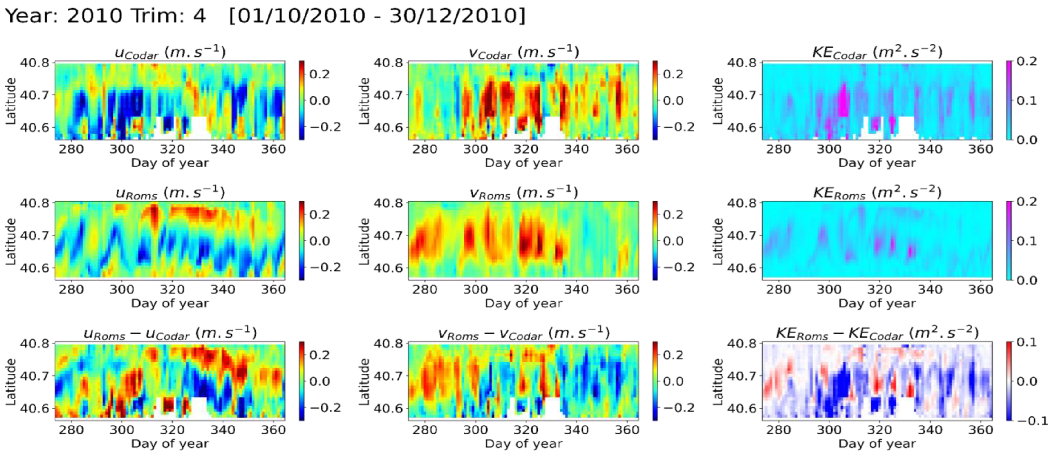
4.2. Hovmöller Diagrams and Selected Areas

The analyses carried out throughout the GoN were repeated on areas of particular interest and investigations along an N–S transect were implemented to describe in detail the circulation and exchanges between the internal and external part of the basin (Figure 4). The selected coastal areas correspond to the area of the fixed hydrological monitoring station (LTER-Mare Chiara) in the northern part of the GoN. An area in front of the HF PORT station, and the area of Castellammare di Stabia, which is in front of the HF CAST station but also in correspondence with the mouth of the river Sarno, represent the most input of fresh waters in the GoN. Finally, an area corresponding to the deep area of the GoN, the Dohrn canyon, was investigated.
The transect goes from Capo Posillipo to Capri, crossing the entire area under investigation (red line in Figure 4). The Hovmöller diagrams were calculated over quarters for the entire study period, the OND quarters for the years of investigation are shown (Figure 5, Figure 6, Figure 7 and Figure 8). We performed this analysis to document the exchanges between the inner and external parts of the GoN. The results describe well the two opposite patterns visible in the northern and southern portions of the transect, as well as the changes in the orientation of the circulation, according to [6]. In general, the comparison of the spatial distributions of the u component and the v component between the model and HFR along the latitudinal section appears to be complex, but show a closer correspondence during the autumn and winter quarters, though there are apparent interannual variabilities presenting large differences in the model performance, showing repeated and abrupt changes of sign, as well as intermingling situations of meridional coherence of the zonal flux, finally the overall pattern was strongly time-dependent.
We can observe that the kinetic energy of the model is lower than the observations, and that the spatial–temporal differences between u and v are noticeable during some monthly periods (October 2009, December 2010, October and December 2011, and October 2012). The November period shows some better agreement, with the bimodal structures in u (distributed from north to south), and the alternance and intensification of v across the section. All the other quarters are available in the Supplementary Material (Figures S4–S6).
The time series of the velocity components and of the kinetic energy are shown for these four areas (averaged from daily to monthly) in Figure 9.
Generally, the coastal area (Figure 9a–c) shows a lower agreement in the v component and higher values of kinetic energy in HFR retrievals; instead, in the area of Canyon Dohrn (Figure 9d), the comparison shows agreement in the velocity components and kinetic energy.
The systematic underestimation of the velocity modulus in the areas closer to the shore could be due to the complete lack of waves modeling and therefore the absence of wave–current interactions. Indeed, waves induced effects particularly important in the near-shore areas, such as the transfer of kinetic energy to the water column due to breaking waves, which are completely missing. The coupling of ROMS with a wave model appears to be an important step for a future version of the model.
Another possibility is that the atmospheric data used to force the model may be the cause of the problem: the ECMWF data used for the evaluation of surface stresses may lack the necessary resolution to describe accurately the near shore areas, where variations in land topography could be strongly affecting the predicted winds, leading to an underestimation of the wind speeds. The ECMWF-interim data used in this work have a 1/8 degree resolution; higher resolution atmospheric data are currently sought to improve the model.
The possibility that the velocity underestimation may be due to an excessive damping caused by the horizontal diffusion has also been examined. The horizontal diffusion coefficient has in fact been set to an arbitrary value well above its theoretical value in order to provide damping of the numerical noise. Numerical tests, not presented here, have shown that this does not appear to be the cause of the velocity underestimation, as halving the diffusion coefficient does not provide any significant increase in the velocity module.
It should also be noticed that the value used in this work, 10 m2 s−1, is smaller than those used in similar applications that have appeared in the literature. For example, [74] modeled the circulation in the GoN with a resolution very similar to the one used here, and adopted a coefficient of 80 m2 s−1 after performing a series of sensitivity experiments.

4.3. Vorticity

Vorticity was calculated in the four locations identifying the north, south, east, and west areas around the center of the GoN (see Figure 4). The analyzes were carried out using a moving average on windows of 10, 30, and 90 days over the primary daily estimates, to identify monthly and three-monthly variability. The results are shown on Figure 10. In general, the observations (HFR) and the model (GNAM) both show a tendency toward negative values/anti-cyclonic circulation. The trimestrial smoothing (90 days, bottom) shows a good agreement, except during the spring period of 2010 when the model was more cyclonic and during the winters 2010 and 2011 when the model shows circulation schemes more anticyclonic with respect to HFR observations. The monthly smoothing (30 days, center) allows us to identify when opposed events occurred, with the tendency of the model to sometimes respond opposedly during some months, compared to the observations (e.g., November 2009, June 2010, or August 2012).

4.4. Hydrological Comparison with LTER-Mare Chiara

The GNAM model was also compared with in situ hydrological parameters of temperatures and salinity retrieved at the LTER-MC fixed monitoring station.
The temperature and salinity time series are reported both on the surface and on the bottom for the years of acquisition 2009–2012, Figure 11. Mean values in the water column are presented too, to represent the contribution of the vertical layers to the average (the Hovmöller diagrams of the vertical profiles of temperature and salinity, for both model and observations, can be consulted in the Supplementary Figure S7). To allow comparisons between the in situ hydrology (weekly sampling) and the GNAM model output (daily outputs), we interpolate the observations with a regular daily time step, and we smooth the model’s output with a running mean of 7 days.
Seasonality of the surface temperature seems to be well reproduced with the monthly peaks from spring to autumn that generally phase well between the model and the observations. When considering the averages in the water column, they indicate a good agreement between the model and the observations during the winter months (from December to March). Then, in general between April and October, the model shows a mean underestimate of around 1 °C to the in situ temperature. On the contrary, the deepest layer presents an overestimation of around 1 °C, and up to 2 °C. Looking at the water column bottom (60 m deep), the variability range of the model is more limited and shows a constant increase in temperature from March to October–November, which is absent from observations where the summer-to-autumn cycle is flatter. While surface stratified layers would reproduce better, the variability driven by vertical and horizontal mixing, ultimately controlling the circulation features budgeting the heat content and freshwater trade-offs, the bottom layer in the model appears to accumulate more/export less the thermal content of the water column. This excessive downward propagation of the surface signal during the restratification could be due to the model vertical mixing that is too high. As a consequence, we should expect an underestimate of the surface currents. This is not the case, as discussed above, which implies that at least partially the bias in the model surface currents are due to the wind forcing and, specifically, to the lack of representation of the coastal orographies in the atmospheric model grid.
In terms of salinity, surface layer frames relatively well the maximum values of salt (≃38 g · k g 1 ) during the autumn and winter periods, even if the variability lacks to reproduce the local disruptions, probably due to the interannual variability of the freshwater runoffs that are not taken into account in the model (climatological data were used here). The decrease of surface salinity is nevertheless visible during the spring periods, even the minimum values (≃37 g · k g 1 ) seen in the in situ observations are not reached. About the variability in the bottom layers, the inter-annual variations seem to generally follow the same trends as the observations. Intra-annual variations are not well reproduced, and in the same way as for temperature, this points out that the model underestimates the horizontal import/export of salty water parcels and their local mixing with the surrounding water mass.

5. Discussion and Conclusions

Multiple platforms collecting measurements of different variables at different scales provide various insights into the model performance. We have evaluated the high-resolution GNAM model using multi-platform observations, HFR, and a fixed monitoring station. The comparison of surface currents retrieved by the HF radar network and obtained by GNAM model on four years (2009–2012) of acquisition was presented. For the same period, a comparison of physical variables of temperature and salinity acquired by a fixed monitoring station located in the GoN was carried out.
The first comparison of surface current components showed a good agreement on the overall period, the monthly correlation coefficient resulted in larger than 0.5 in winter (January–March) for both components. With a maximum value in January 2010 of 0.973 for the u component and 0.917 for the v component, respectively. In all years of comparison, a good agreement was found in the winter months and a lower agreement in those close to the summer, mainly for the meridional component (v). This agreement was found also in the quarter analysis of the years, confirming the good representation of the model. The results show the reliability of the ROMS model to solve the surface dynamics and reproducing the seasonal patterns typical of the study area [6,10,25,26].
The results of the Hovmöller diagrams reproduce the structures and changes in direction of surface currents observed in a previous study [6], showing more complexity in the summer period. The analysis over quarters reproduces the two opposite patterns in the northern and southern portions of the transect, as well as the changes in the orientation of the circulation.
Even though the coastal ocean forecasting system presented here does not currently employ the assimilation of ocean variables, ROMS contains the tangent linear and adjoint formulations necessary for advanced assimilation techniques such as 3DVAR and 4DVAR data assimilation methods. Further improvement of the forecast may be achieved by assimilating data from the acoustic Doppler current profiler (ADCP) and HFR measurements, and the coastal model presented here lays the foundation for such improvements [75].
We show in our study that the surface temperature reproduces a seasonal and inter-annual cycle in good agreement with the observations, while the time series at the bottom of the water column at the LTER-MC coastal station shows a warming cycle that anticipates the observations, every year, and could be due to the mixing scheme implementation that could be modified with stronger turbulent diffusion rates. In general, both vertical and horizontal mixing are difficult to model properly in their amplitudes and dynamics, which could render complex the right representation of the heat budget in such a coastal area. This should require more direct in situ observations of the local turbulence to allow a finer tuning of the model.
In the recent joint studies about the marine ecosystem of the GoN [76], it has been shown that the hydrology at the LTER-MC coastal station was marked by a specific cycle in salinity via the establishment of the surface freshwater layer in spring. This fresh feature appears to be relatively well reproduced in the model with the minimum of surface salinity reached in April–May. Given that the model does not take in account the fresh runoffs but only the main rivers flow, the agreement in the variability for both model and observations suggest a realistic representation of the local horizontal advection of the rivers’ freshwater discharge (e.g., Sarno and Volturno rivers). The authors emphasized the observed delay between the maximum of rain (March) and the minimum of salinity (May–June), which could be driven by the mesoscale activity mitigating the inshore and offshore exchanges, as it is suggested by the vorticity index showing variations at the monthly time scale.
This index represents a very informative proxy to infer the local advection of the various fresh and salty inputs in the GoN by mesoscale features, as it was shown that the GoN area was prompt to be influenced by such structures [77]. A positive/cyclonic mode could favor the northward–westward export and distribution of the fresh runoffs from the Sarno river (located in the east corner of the GoN) along the coastline. On the contrary, a negative/anti-cyclonic mode should lead to another pattern of circulation, by redistributing the coastal runoffs more southward and towards the gulf’s center. Our study highlights this inner feature of the GoN, that should be driven by surface wind forcing. The surface response to such forcing could be then determined with the help of the GNAM model, that should allow to disentangle the respective influence of large-scale, mesoscale, and sub-mesoscale processes in setting the GoN surface and subsurface hydrology, through the trade offs with the open Tyrrhenian Sea [6,10].
During the post-summer and autumn season, the local hydrological cycle was characterized by a salty water layer at mid-depth in September–November, favorably hosting diffusive processes on the vertical through the establishment of a salt-fingering regime [23,63]. This represents a possibly significant input of salty flow, whose importance for biological communities is still to be assessed. The GNAM model is consequently of interest here, given the good agreement between the seasonal comparisons at this particular period, and the possibility of tracking back virtual particles as it includes implemented Lagrangian tools. More generally, the model paves the way for studies dedicated to the connectivity between the various areas of the GoN.

Supplementary Materials

The following supporting information can be downloaded at: https://www.mdpi.com/article/10.3390/jmse10081044/s1, Table S1: List of the acronyms used in the text. Figure S1: Average maps of velocities (components u, v) and kinetic energy over the area covered by the Codar network (quality > 70%) in the Gulf of Naples, compared to the GNAM model, during the 1st trimestrial period of each year (2009 to 2012). For each grid point a correlation coefficient is calculated between the trimestrial time series of the velocity components, between numerical model and observations. Figure S2: Average maps of velocities (components u, v) and kinetic energy over the area covered by the Codar network (quality > 70%) in the Gulf of Naples, compared to the GNAM model, during the 2nd trimestrial period of each year (2009 to 2012). For each grid point a correlation coefficient is calculated between the trimestrial time series of the velocity components, between numerical model and observations. Figure S3: Average maps of velocities (components u, v) and kinetic energy over the area covered by the Codar network (quality > 70%) in the Gulf of Naples, compared to the GNAM model, during the 3rd trimestrial period of each year (2009 to 2012). For each grid point a correlation coefficient is calculated between the trimestrial time series of the velocity components, between numerical model and observations. Figure S4: Hovmöller diagrams of the zonal and meridional component of the surface current (cm/s) and kinetic energy measured by the HFR and obtained from model simulation over the transect for the quarter JFM in 2009 (a), 2010 (b), 2011 (c), and 2012 (d). Figure S5: Hovmöller diagrams of the zonal and meridional component of the surface current (cm/s) and kinetic energy measured by the HFR and obtained from model simulation over the transect for the quarter AMJ in 2009 (a), 2010 (b), 2011 (c), and 2012 (d). Figure S6: Hovmöller diagrams of the zonal and meridional component of the surface current (cm/s) and kinetic energy measured by the HFR and obtained from model simulation over the transect for the quarter JAS in 2009 (a), 2010 (b), 2011 (c), and 2012 (d). Figure S7: Hovmöller diagrams of the vertical profiles of temperature and salinity of the GNAM model (daily) at the LTER-MC coastal station, compared to the in situ data (weekly). Isotherms levels are indicated by contours every 0.5 °C from 16 °C to 29 °C. Isohalines levels are indicated by contours every 0.1 g · k g 1 from 37.2 to 38.2 g · k g 1 .

Author Contributions

Conceptualization, F.K., S.S., D.I., E.Z. and D.C.; Data curation, F.K., S.S. and V.B.; Formal analysis, F.K., S.S. and D.C.; Funding acquisition, E.Z. and D.C.; Investigation, F.K., S.S. and E.Z.; Methodology, F.K., S.S., D.I. and D.C.; Project administration, D.C.; Resources, D.C.; Software, F.K., S.S. and V.B.; Supervision, D.I., E.Z. and D.C.; Validation, F.K., S.S. and V.B.; Visualization, F.K. and S.S.; Writing—original draft, F.K. and S.S.; Writing—review and editing, F.K., S.S., V.B., D.I., E.Z. and D.C. All authors have read and agreed to the published version of the manuscript.

Funding

This research was partly funded by the 2017 PRIN project EMME (Exploring the fate of Mediterranean microplastic: from distribution pathways to biological effects), funded by the Italian Ministry for Research (grant agreement No. 2017WERYZP). S.S. is supported by Stazione Zoologica Anton Dohrn PON PRIMA (project CIR01_00029).

Acknowledgments

The authors would like to thank Fabio Conversano, Marco Cannavacciuolo, Augusto Passarelli, Ferdinando Tramontano, Giancluca Zazo and the crew of the R/V Vettoria, for sampling and data collection at sea. We also thank the Marine Research Infrastructure of the Stazione Zoologica for acquiring, processing, and managing the hydrological data, and the entire LTER-MC Team for continued collaboration in the project.

Conflicts of Interest

The authors declare no conflict of interest.

References

  1. Fox-Kemper, B.; Adcroft, A.; Böning, C.W.; Chassignet, E.P.; Curchitser, E.; Danabasoglu, G.; Eden, C.; England, M.H.; Gerdes, R.; Greatbatch, R.J.; et al. Challenges and Prospects in Ocean Circulation Models. Front. Mar. Sci. 2019, 6, 65. [Google Scholar] [CrossRef]
  2. Mourre, B.; Aguiar, E.; Juza, M.; Hernandez-Lasheras, J.; Reyes, E.; Heslop, E.; Escudier, R.; Cutolo, E.; Ruiz, S.; Mason, E.; et al. Assessment of High-Resolution Regional Ocean Prediction Systems Using Multi-Platform Observations: Illustrations in the Western Mediterranean Sea. New Front. Oper. Oceanogr. 2018, 663–694. [Google Scholar] [CrossRef] [Green Version]
  3. Capotondi, A.; Jacox, M.; Bowler, C.; Kavanaugh, M.; Lehodey, P.; Barrie, D.; Brodie, S.; Chaffron, S.; Cheng, W.; Dias, D.F.; et al. Observational Needs Supporting Marine Ecosystems Modeling and Forecasting: From the Global Ocean to Regional and Coastal Systems. Front. Mar. Sci. 2019, 6, 623. [Google Scholar] [CrossRef] [Green Version]
  4. Ferla, M.; Nardone, G.; Orasi, A.; Picone, M.; Falco, P.; Zambianchi, E. Sea Monitoring Networks. In Measurement for the Sea; Springer: Cham, Switzerland, 2022; pp. 211–235. [Google Scholar]
  5. Davidson, F.; Alvera-Azcárate, A.; Barth, A.; Brassington, G.B.; Chassignet, E.P.; Clementi, E.; De Mey-Frémaux, P.; Divakaran, P.; Harris, C.; Hernandez, F.; et al. Synergies in Operational Oceanography: The Intrinsic Need for Sustained Ocean Observations. Front. Mar. Sci. 2019, 6, 450. [Google Scholar] [CrossRef] [Green Version]
  6. Cianelli, D.; Falco, P.; Iermano, I.; Mozzillo, P.; Uttieri, M.; Buonocore, B.; Zambardino, G.; Zambianchi, E. Inshore/offshore water exchange in the Gulf of Naples. J. Mar. Syst. 2015, 145, 37–52. [Google Scholar] [CrossRef]
  7. O’Donncha, F.; Hartnett, M.; Nash, S.; Ren, L.; Ragnoli, E. Characterizing observed circulation patterns within a bay using HF radar and numerical model simulations. J. Mar. Syst. 2015, 142, 96–110. [Google Scholar] [CrossRef]
  8. Hernandez-Lasheras, J.; Mourre, B.; Orfila, A.; Santana, A.; Reyes, E.; Tintoré, J. Evaluating high-frequency radar data assimilation impact in coastal ocean operational modelling. Ocean Sci. 2021, 17, 1157–1175. [Google Scholar] [CrossRef]
  9. Edwards, C.A.; Moore, A.M.; Hoteit, I.; Cornuelle, B.D. Regional Ocean Data Assimilation. Annu. Rev. Mar. Sci. 2015, 7, 21–42. [Google Scholar] [CrossRef] [Green Version]
  10. Iermano, I.; Moore, A.; Zambianchi, E. Impacts of a 4-dimensional variational data assimilation in a coastal ocean model of southern Tyrrhenian Sea. J. Mar. Syst. 2016, 154, 157–171. [Google Scholar] [CrossRef]
  11. Kourafalou, V.H.; De Mey, P.; Le Hénaff, M.; Charria, G.; Edwards, C.A.; He, R.; Herzfeld, M.; Pascual, A.; Stanev, E.V.; Tintoré, J.; et al. Coastal Ocean Forecasting: System integration and evaluation. J. Oper. Oceanogr. 2015, 8, s127–s146. [Google Scholar] [CrossRef] [Green Version]
  12. Lorente, P.; Aguiar, E.; Bendoni, M.; Berta, M.; Brandini, C.; Cáceres-Euse, A.; Capodici, F.; Cianelli, D.; Ciraolo, G.; Corgnati, L.; et al. Coastal high-frequency radars in the Mediterranean—Part 1: Status of operations and a framework for future development. Ocean Sci. 2022, 18, 761–795. [Google Scholar] [CrossRef]
  13. Reyes, E.; Aguiar, E.; Bendoni, M.; Berta, M.; Brandini, C.; Cáceres-Euse, A.; Capodici, F.; Cardin, V.; Cianelli, D.; Ciraolo, G.; et al. Coastal high-frequency radars in the Medi-terranean—Part 2: Applications in support of science priorities and societal needs. Ocean Sci. 2022, 18, 797–837. [Google Scholar] [CrossRef]
  14. Lorente, P.; Piedracoba, S.; Sotillo, M.; Aznar, R.; Amo-Balandron, A.; Pascual, A.; Soto-Navarro, J.; Alvarez-Fanjul, E. Characterizing the surface circulation in Ebro Delta (NW Mediterranean) with HF radar and modeled current data. J. Mar. Syst. 2016, 163, 61–79. [Google Scholar] [CrossRef]
  15. Ruiz-Parrado, I.; Genua-Olmedo, A.; Reyes, E.; Mourre, B.; Rotllán, P.; Lorente, P.; García-Sotillo, M.; Tintoré, J. Coastal ocean variability related to the most extreme Ebro River discharge over the last 15 years, in: Copernicus Marine Service Ocean State Report, Issue 4. J. Oper. Oceanogr. 2020, 13 (Suppl. S1), 160–165. [Google Scholar] [CrossRef]
  16. Aguiar, E.; Mourre, B.; Juza, M.; Reyes, E.; Hernández-Lasheras, J.; Cutolo, E.; Mason, E.; Tintoré, J. Multi-platform model assessment in the Western Mediterranean Sea: Impact of downscaling on the surface circulation and mesoscale activity. Ocean Dyn. 2019, 70, 273–288. [Google Scholar] [CrossRef] [Green Version]
  17. Lorente, P.; Lin-Ye, J.; García-León, M.; Reyes, E.; Fernandes, M.; Sotillo, M.G.; Espino, M.; Ruiz, M.I.; Gracia, V.; Perez, S.; et al. On the Performance of High Frequency Radar in the Western Mediterranean During the Record-Breaking Storm Gloria. Front. Mar. Sci. 2021, 8, 645762. [Google Scholar] [CrossRef]
  18. Sotillo, M.G.; Mourre, B.; Mestres, M.; Lorente, P.; Aznar, R.; García-León, M.; Liste, M.; Santana, A.; Espino, M.; Álvarez, E. Evaluation of the Operational CMEMS and Coastal Downstream Ocean Forecasting Services During the Storm Gloria (January 2020). Front. Mar. Sci. 2021, 8, 644525. [Google Scholar] [CrossRef]
  19. Révelard, A.; Reyes, E.; Mourre, B.; Hernández-Carrasco, I.; Rubio, A.; Lorente, P.; Fernández, C.D.L.; Mader, J.; Álvarez-Fanjul, E.; Tintoré, J. Sensitivity of Skill Score Metric to Validate Lagrangian Simulations in Coastal Areas: Recommendations for Search and Rescue Applications. Front. Mar. Sci. 2021, 8, 630388. [Google Scholar] [CrossRef]
  20. Vilibic, I.; Šepi’c, J.; Mihanovi’c, H.; Kalini´c, H.; Cosoli, S.; Janekovic, I.; Žagar, N.; Jesenko, B.; Tudor, M.; Dadic, V.; et al. Self-Organizing Maps-based ocean currents forecasting system. Sci. Rep. 2016, 6, 22924. [Google Scholar] [CrossRef] [PubMed]
  21. Lorente, P.; García-Sotillo, M.; Amo-Baladrón, A.; Aznar, R.; Levier, B.; Sánchez-Garrido, J.C.; Sammartino, S.; de Pas-cualCollar, Á.; Reffray, G.; Toledano, C.; et al. Skill assessment of global, regional, and coastal circu-lation forecast models: Evaluating the benefits of dynamical downscaling in IBI (Iberia–Biscay–Ireland) surface waters. Ocean Sci. 2019, 15, 967–996. [Google Scholar] [CrossRef] [Green Version]
  22. Del Gaizo, G.; Russo, L.; Abagnale, M.; Buondonno, A.; Furia, M.; Saviano, S.; Vargiu, M.; Conversano, F.; Margiotta, F.; Saggiomo, M.; et al. An autumn biodiversity survey on heterotrophic and mixotrophic protists along a coast-to-offshore transect in the Gulf of Naples (Italy). Adv. Oceanogr. Limnol. 2021, 12, 74–82. [Google Scholar] [CrossRef]
  23. Kokoszka, F.; Iudicone, D.; Zingone, A.; Saggiomo, V.; D’Alcalá, M.R.; Conversano, F. A note about density staircases in the Gulf of Naples: 20 years of persistent weak salt-fingering layers in a coastal area. Adv. Oceanogr. Limnol. 2021, 12, 65–73. [Google Scholar] [CrossRef]
  24. Ciannelli, L.; Cannavacciuolo, A.; Konstandinidis, P.; Mirasole, A.; Wong-Ala, J.A.T.K.; Guerra, M.T.; D’Ambra, I.; Riginella, E.; Cianelli, D. Ichthyoplankton assemblages and physical characteristics of two submarine canyons in the south central Tyrrhenian Sea. Fish. Oceanogr. 2022, 1–17. [Google Scholar] [CrossRef]
  25. Cianelli, D.; D’Alelio, D.; Uttieri, M.; Sarno, D.; Zingone, A.; Zambianchi, E.; Ribera d’Alcalà, M. Disentangling physical and biological drivers of phytoplankton dynamics in a coastal system. Sci. Rep. 2017, 7, 15868. [Google Scholar] [CrossRef] [PubMed] [Green Version]
  26. Menna, M.; Mercatini, A.; Uttieri, M.; Buonocore, B.; Zambianchi, E. Wintertime transport processes in the Gulf of Naples investigated by HF radar measurements of surface currents. Nuovo Cimento. 2007, 30, 605–622. [Google Scholar]
  27. de Ruggiero, P.; Esposito, G.; Napolitano, E.; Iacono, R.; Pierini, S.; Zambianchi, E. Modelling the marine circulation of the Campania coastal system (Tyrrhenian Sea) for the year 2016: Analysis of the dynamics. J. Mar. Syst. 2020, 210, 103388. [Google Scholar] [CrossRef]
  28. Saviano, S.; Esposito, G.; Di Lemma, R.; de Ruggiero, P.; Zambianchi, E.; Pierini, S.; Falco, P.; Buonocore, B.; Cianelli, D.; Uttieri, M. Wind Direction Data from a Coastal HF Radar System in the Gulf of Naples (Central Mediterranean Sea). Remote Sens. 2021, 13, 1333. [Google Scholar] [CrossRef]
  29. Saviano, S.; Kalampokis, A.; Zambianchi, E.; Uttieri, M. A year-long assessment of wave measurements retrieved from an HF radar network in the Gulf of Naples (Tyrrhenian Sea, Western Mediterranean Sea). J. Oper. Oceanogr. 2019, 12, 1–15. [Google Scholar] [CrossRef]
  30. Saviano, S.; Cianelli, D.; Zambianchi, E.; Conversano, F.; Uttieri, M. An Integrated Reconstruction of the Multiannual Wave Pattern in the Gulf of Naples (South-Eastern Tyrrhenian Sea, Western Mediterranean Sea). J. Mar. Sci. Eng. 2020, 8, 372. [Google Scholar] [CrossRef]
  31. Hatzaki, M.; Flocas, H.A.; Simmonds, I.; Kouroutzoglou, J.; Keay, K.; Rudeva, I. Seasonal Aspects of an Objective Climatology of Anticyclones Affecting the Mediterranean. J. Clim. 2014, 27, 9272–9289. [Google Scholar] [CrossRef]
  32. Krauzig, N.; Falco, P.; Zambianchi, E. Contrasting surface warming of a marginal basin due to large-scale climatic patterns and local forcing. Sci. Rep. 2020, 10, 17648. [Google Scholar] [CrossRef] [PubMed]
  33. Saviano, S.; De Leo, F.; Besio, G.; Zambianchi, E.; Uttieri, M. HF Radar Measurements of Surface Waves in the Gulf of Naples (Southeastern Tyrrhenian Sea): Comparison With Hindcast Results at Different Scales. Front. Mar. Sci. 2020, 7, 492. [Google Scholar] [CrossRef]
  34. Saviano, S.; Biancardi, A.A.; Uttieri, M.; Zambianchi, E.; Cusati, L.A.; Pedroncini, A.; Contento, G.; Cianelli, D. Sea Storm Analysis: Evaluation of Multiannual Wave Parameters Retrieved from HF Radar and Wave Model. Remote Sens. 2022, 14, 1696. [Google Scholar] [CrossRef]
  35. Haidvogel, D.B.; Arango, H.; Budgell, W.P.; Cornuelle, B.D.; Curchitser, E.; Di Lorenzo, E.; Fennel, K.; Geyer, W.R.; Hermann, A.J.; Lanerolle, L.; et al. Ocean forecasting in terrain-following coordinates: Formulation and skill assessment of the Regional Ocean Modeling System. J. Comput. Phys. 2008, 227, 3595–3624. [Google Scholar] [CrossRef]
  36. Lin, X.; Yan, X.-H.; Jiang, Y.; Zhang, Z. Performance assessment for an operational ocean model of the Taiwan Strait. Ocean Model. 2016, 102, 27–44. [Google Scholar] [CrossRef]
  37. Lu, W.; Jiang, Y.; Lin, J. Modeling Propagation of 2011 Honshu Tsunami. Eng. Appl. Comput. Fluid Mech. 2013, 7, 507–518. [Google Scholar] [CrossRef] [Green Version]
  38. Lu, W.; Yan, X.-H.; Han, L.; Jiang, Y. One-dimensional ocean model with three types of vertical velocities: A case study in the South China Sea. Ocean Dyn. 2017, 67, 253–262. [Google Scholar] [CrossRef]
  39. Zhou, F.; Chai, F.; Huang, D.; Xue, H.; Chen, J.; Xiu, P.; Xuan, J.; Li, J.; Zeng, D.; Ni, X.; et al. Investigation of hypoxia off the Changjiang Estuary using a coupled model of ROMS-CoSiNE. Prog. Oceanogr. 2017, 159, 237–254. [Google Scholar] [CrossRef]
  40. Gan, J.; Li, L.; Wang, D.; Guo, X. Interaction of a river plume with coastal upwelling in the northeastern South China Sea. Cont. Shelf Res. 2009, 29, 728–740. [Google Scholar] [CrossRef]
  41. Gan, J.; Liu, Z.; Hui, C.R. A Three-Layer Alternating Spinning Circulation in the South China Sea. J. Phys. Oceanogr. 2016, 46, 2309–2315. [Google Scholar] [CrossRef] [Green Version]
  42. Dobricic, S.; Pinardi, N.; Adani, M.; Tonani, M.; Fratianni, C.; Bonazzi, A.; Fernandez, V. Daily oceanographic analyses by Mediterranean Forecasting System at the basin scale. Ocean Sci. 2007, 3, 149–157. [Google Scholar] [CrossRef] [Green Version]
  43. Marchesiello, P.; McWilliams, J.C.; Shchepetkin, A. Open boundary conditions for long-term integration of regional oceanic models. Ocean Model. 2001, 3, 1–20. [Google Scholar] [CrossRef]
  44. Large, W.G.; McWilliams, J.C.; Doney, S. Oceanic vertical mixing: A review and a model with a nonlocal boundary layer parameterization. Rev. Geophys. 1994, 32, 363–403. [Google Scholar] [CrossRef] [Green Version]
  45. Fairall, C.; Bradley, E.F.; Rogers, D.P.; Edson, J.B.; Young, G.S. Bulk parameterization of air-sea fluxes for Tropical Ocean-Global Atmosphere Coupled-Ocean Atmosphere Response Experiment. J. Geophys. Res. Earth Surf. 1996, 101, 3747–3764. [Google Scholar] [CrossRef]
  46. Dee, D.P.; Uppala, S.M.; Simmons, A.J.; Berrisford, P.; Poli, P.; Kobayashi, S.; Andrae, U.; Balmaseda, M.A.; Balsamo, G.; Bauer, P.; et al. The ERA-Interim reanalysis: Configuration and performance of the data assimilation system. Q. J. R. Meteorol. Soc. 2011, 137, 553–597. [Google Scholar] [CrossRef]
  47. Barrick, D.; Fernandez, V.; Ferrer, M.I.; Whelan, C.; Breivik, Ø. A short-term predictive system for surface currents from a rapidly deployed coastal HF radar network. Ocean Dyn. 2012, 62, 725–740. [Google Scholar] [CrossRef]
  48. Gurgel, K.-W.; Antonischki, G.; Essen, H.-H.; Schlick, T. Wellen Radar (WERA): A new ground-wave HF radar for ocean remote sensing. Coast. Eng. 1999, 37, 219–234. [Google Scholar] [CrossRef]
  49. Kaplan, D.D.; Lekien, F. Spatial interpolation and filtering of surface current data based on open-boundary modal analysis. J. Geophys. Res. Earth Surf. 2007, 112, 68. [Google Scholar] [CrossRef] [Green Version]
  50. Molcard, A.; Poulain, P.; Forget, P.; Griffa, A.; Barbin, Y.; Gaggelli, J.; De Maistre, J.; Rixen, M. Comparison between VHF radar observations and data from drifter clusters in the Gulf of La Spezia (Mediterranean Sea). J. Mar. Syst. 2009, 78, S79–S89. [Google Scholar] [CrossRef]
  51. Paduan, J.D.; Washburn, L. High-Frequency Radar Observations of Ocean Surface Currents. Annu. Rev. Mar. Sci. 2013, 5, 115–136. [Google Scholar] [CrossRef] [PubMed] [Green Version]
  52. Uttieri, M.; Cianelli, D.; Nardelli, B.B.; Buonocore, B.; Falco, P.; Colella, S.; Zambianchi, E. Multiplatform observation of the surface circulation in the Gulf of Naples (Southern Tyrrhenian Sea). Ocean Dyn. 2011, 61, 779–796. [Google Scholar] [CrossRef]
  53. Roarty, H.; Cook, T.; Hazard, L.; George, D.; Harlan, J.; Cosoli, S.; Wyatt, L.; Alvarez Fanjul, E.; Terrill, E.; Otero, M.; et al. The Global High Frequency Radar Network. Front. Mar. Sci. 2019, 6, 164. [Google Scholar] [CrossRef]
  54. Lorente, P.; Piedracoba, S.; Sotillo, M.G.; Álvarez-Fanjul, E. Long-Term Monitoring of the Atlantic Jet through the Strait of Gibraltar with HF Radar Observations. J. Mar. Sci. Eng. 2019, 7, 3. [Google Scholar] [CrossRef] [Green Version]
  55. Kuang, L.; Blumberg, A.F.; Georgas, N. Assessing the fidelity of surface currents from a coastal ocean model and HF radar using drifting buoys in the Middle Atlantic Bight. Ocean Dyn. 2012, 62, 1229–1243. [Google Scholar] [CrossRef]
  56. Barth, A.; Weisberg, R.H.; Alvera-Azcárate, A. Assimilation of high-frequency radar currents in a nested model of the West Florida Shelf. J. Geophys. Res. Earth Surf. 2008, 113, 56. [Google Scholar] [CrossRef] [Green Version]
  57. Breivik, Ø.; Sætra, Ø. Real time assimilation of HF radar currents into a coastal ocean model. J. Mar. Syst. 2001, 28, 161–182. [Google Scholar] [CrossRef] [Green Version]
  58. Crombie, D.D. Doppler Spectrum of Sea Echo at 13.56 Mc./s. Nature 1955, 175, 681–682. [Google Scholar] [CrossRef]
  59. Barrick, D.E. Extraction of wave parameters from measured HF radar sea-echo Doppler spectra. Radio Sci. 1977, 12, 415–424. [Google Scholar] [CrossRef]
  60. Paduan, J.D.; Rosenfeld, L.K. Remotely sensed surface currents in Monterey Bay from shore-based HF radar (Coastal Ocean Dynamics Application Radar). J. Geophys. Res. Earth Surf. 1996, 101, 20669–20686. [Google Scholar] [CrossRef]
  61. Paduan, J.; Graber, H. Introduction to High-Frequency Radar: Reality and Myth. Oceanography 1997, 10, 36–39. [Google Scholar] [CrossRef]
  62. Barrick, D.; Lipa, B. Correcting for distorted antenna patterns in CODAR ocean surface measurements. IEEE J. Ocean. Eng. 1986, 11, 304–309. [Google Scholar] [CrossRef]
  63. Falco, P.; Buonocore, B.; Cianelli, D.; De Luca, L.; Giordano, A.; Iermano, I.; Kalampokis, A.; Saviano, S.; Uttieri, M.; Zambardino, G.; et al. Dynamics and sea state in the Gulf of Naples: Potential use of high-frequency radar data in an operational oceanographic context. J. Oper. Oceanogr. 2016, 9 (Suppl. S1), s33–s45. [Google Scholar] [CrossRef] [Green Version]
  64. Zingone, A.; Montresor, M.; Marino, D. Summer Phytoplankton Physiognomy in Coastal Waters of the Gulf of Naples. Mar. Ecol. 1990, 11, 157–172. [Google Scholar] [CrossRef]
  65. McDougall, T.J.; Barker, P.M. Getting started with TEOS-10 and the Gibbs Seawater (GSW) oceanographic toolbox. Scor/Iapso WG 2011, 127, 1–28. [Google Scholar]
  66. White, M.A.; Heywood, K.J. Seasonal and interannual changes in the North Atlantic subpolar gyre from Geosat and TOPEX/POSEIDON altimetry. J. Geophys. Res. Earth Surf. 1995, 100, 24931–24941. [Google Scholar] [CrossRef]
  67. Zhai, X.; Greatbatch, R.J.; Kohlmann, J.-D. On the seasonal variability of eddy kinetic energy in the Gulf Stream region. Geophys. Res. Lett. 2008, 35, 33. [Google Scholar] [CrossRef] [Green Version]
  68. Jouanno, J.; Sheinbaum, J.; Barnier, B.; Molines, J.M.; Candela, J. Seasonal and Interannual Modulation of the Eddy Kinetic Energy in the Caribbean Sea. J. Phys. Oceanogr. 2012, 42, 2041–2055. [Google Scholar] [CrossRef]
  69. Rieck, J.K.; Böning, C.W.; Greatbatch, R.J.; Scheinert, M. Seasonal variability of eddy kinetic energy in a global high-resolution ocean model. Geophys. Res. Lett. 2015, 42, 9379–9386. [Google Scholar] [CrossRef] [Green Version]
  70. Kang, D.; Curchitser, E.N.; Rosati, A. Seasonal Variability of the Gulf Stream Kinetic Energy. J. Phys. Oceanogr. 2016, 46, 1189–1207. [Google Scholar] [CrossRef]
  71. Kang, D.; Curchitser, E.N. Energetics of Eddy–Mean Flow Interactions in the Gulf Stream Region. J. Phys. Oceanogr. 2015, 45, 1103–1120. [Google Scholar] [CrossRef]
  72. Ferrari, R.; Wunsch, C. Ocean Circulation Kinetic Energy: Reservoirs, Sources, and Sinks. Annu. Rev. Fluid Mech. 2009, 41, 253–282. [Google Scholar] [CrossRef] [Green Version]
  73. Vallis, G.K. Atmospheric and Oceanic Fluid Dynamics: Fundamentals and Large-Scale Circulation; Cambridge University Press: Cambridge, UK, 2006. [Google Scholar] [CrossRef]
  74. de Ruggiero, P.; Napolitano, E.; Iacono, R.; Pierini, S. A high-resolution modelling study of the circulation along the Campania coastal system, with a special focus on the Gulf of Naples. Cont. Shelf Res. 2016, 122, 85–101. [Google Scholar] [CrossRef]
  75. Solano, M.; Canals, M.; Leonardi, S. Development and validation of a coastal ocean forecasting system for Puerto Rico and the U.S. virgin islands. J. Ocean Eng. Sci. 2018, 3, 223–236. [Google Scholar] [CrossRef]
  76. Iermano, I.; Liguori, G.; Iudicone, D.; Nardelli, B.B.; Colella, S.; Zingone, A.; Saggiomo, V.; D’Alcalà, M.R. Filament formation and evolution in buoyant coastal waters: Observation and modelling. Prog. Oceanogr. 2012, 106, 118–137. [Google Scholar] [CrossRef]
  77. Kokoszka, F.; Le Roux, B.; Iudicone, D.; Conversano, F.; Ribera d’Alcalá, M. Long-term variability of the coastal ocean stratification in the Gulf of Naples: Two decades of monitoring the marine ecosystem at the LTER-MC site, between land and open Mediterranean sea. Earth Space Sci. Open Arch. 2022, 43. under review. [Google Scholar] [CrossRef]
Figure 1. Map of the Gulf of Naples (southeastern Tyrrhenian Sea, western Mediterranean Sea; see inset) with the locations of the three HF radar sites (stars, see Section 3.2) and LTER-MC (pink point, see Section 3.3). The thin bathymetric contours indicate the 50, 200, 300, and 400 m deep isobaths; thick ones indicate the 100, 500, 1000, and 2000 m deep isobaths.
Jmse 10 01044 g001
Figure 2. (a) ROMS grid covering the whole Tyrrhenian Sea, with a 2 km resolution. (b) ROMS finer grid, covering the Campania coast with a 500 m resolution. (c) Spatial coverage of CODAR data in the year 2012. The area of CODAR domain characterized by a coverage of at list 90% (black dotted line) is highlighted.
Jmse 10 01044 g002
Figure 3. Average maps of velocities (components u, v) and kinetic energy over the area covered by the Codar network (quality > 70%) in the Gulf of Naples, compared to the GNAM model, during the 4th trimestrial period of each year (a) 2009, (b) 2010, (c) 2011 and (d) 2012. For each grid point a correlation coefficient is calculated between the trimestrial time series of the velocity components, between numerical model and observations.
Jmse 10 01044 g003
Figure 4. Common grid points between HFR observations and GNAM model in the Gulf of Naples (coastline in black). Benchmark’s areas are indicated in red (zones of interest and latitudinal section) and green (boxes to infer the vorticity index). The LTER-MC coastal station is located with the cross.
Jmse 10 01044 g004
Figure 5. Hovmöller diagrams of the zonal and meridional component of the surface current (cm/s) and kinetic energy measured by the HFR and obtained from model simulation over the transect for the quarter OND in 2009.
Jmse 10 01044 g005
Figure 6. Hovmöller diagrams of the zonal and meridional component of the surface current (cm/s) and kinetic energy measured by the HFR and obtained from model simulation over the transect for the quarter OND in 2010.
Jmse 10 01044 g006
Figure 7. Hovmöller diagrams of the zonal and meridional component of the surface current (cm/s) and kinetic energy measured by the HFR and obtained from model simulation over the transect for the quarter OND in 2011.
Jmse 10 01044 g007
Figure 8. Hovmöller diagrams of the zonal and meridional component of the surface current (cm/s) and kinetic energy measured by the HFR and obtained from model simulation over the transect for the quarter OND in 2012.
Jmse 10 01044 g008
Figure 9. Time series of the monthly averaged velocities (components u, v, and module) and their associated kinetic energy at the four specific areas: (a) Marechiara, (b) Portici, (c) Castellammare and (d) Canyon Dohrn. Red: HFR observations; blue: GNAM model.
Jmse 10 01044 g009
Figure 10. Vorticity index, smoothed with a running-average window of 10, 30, and 90 days (top, middle, and bottom, respectively). Primary daily values are indicated with the dots in background. Red: HFR observations; blue: ROMS model.
Jmse 10 01044 g010
Figure 11. Time series of conservative temperature T (°C) and absolute salinity S ( g · k g 1 ) at the LTER-MC coastal station, at the surface, averaged into the water column, and at the bottom (60 m deep). Red: LTER-MC observations; blue: GNAM model.
Jmse 10 01044 g011
Table 1. In table are reported the ρ of GNAM and HFR current component (u, v) in the GoN (with 70% of coverage in HFR data).
Year2009201020112012
Monthsuvuvuvuv
Jan0.820.710.970.920.510.560.890.79
Feb0.620.840.680.660.70.830.650.76
Mar0.810.910.870.790.880.840.810.57
Apr0.830.910.760.810.770.250.780.73
May0.580.430.870.720.780.690.650.62
Jun0.380.720.760.470.600.510.220.57
Jul0.670.690.740.500.170.680.480.47
Aug0.680.140.510.390.760.450.670.27
Sep0.810.490.640.530.570.200.320.39
Oct0.41-0.060.580.600.570.0080.570.85
Nov0.310.340.760.780.520.470.730.84
Dec0.710.90.780.630.880.650.770.89
Mean0.640.750.640.630.580.660.510.65
Publisher’s Note: MDPI stays neutral with regard to jurisdictional claims in published maps and institutional affiliations.

