Discrete Element Simulation of the Macro-Meso Mechanical Behaviors of Gas-Hydrate-Bearing Sediments under Dynamic Loading

Abstract

Under the action of dynamic loadings such as earthquakes and volcanic activities, the mechanical properties of gas-hydrate-bearing sediments will deteriorate, leading to a decrease in the stability of hydrate reservoirs and even inducing geological disasters such as submarine landslides. In order to study the effect of dynamic loading on the mechanical properties of hydrate sediments, triaxial compression tests of numerical specimens were carried out by using particle flow code (PFC2D), and the macro-meso mechanical behaviors of specimens were investigated. The results show that the loading frequency has a small effect on the stiffness of the hydrate sediment, while it has a large effect on the peak strength. The peak strength increases and then decreases with the increase in loading frequency. Under the same loading frequency, the peak strength of the hydrate sediment increases with the increase in loading amplitude, and the stiffness of the specimen decreases with the increase in loading amplitude. The maximum shear expansion of the specimen changes with the movement of the phase change point and the rearrangement of the particles. The maximum shear expansion of the specimen changes with the movement of the phase change point and the change of the bearing capacity of the particles after the rearrangement, and the more forward the phase change point is, the stronger the bearing capacity of the specimen in the plastic stage. The shear dilatancy angle and the shear dilatancy amount both increase linearly with the increase in loading amplitude. The influence of loading frequency and amplitude on the contact force chain, displacement, crack expansion, and the number of cementation damage inside the sediment is mainly related to the average axial stress to which the specimen is subjected, and the number of cracks and cementation damage of the sediment specimen increases with the increase in the average axial stress to which the sediment specimen is subjected. As the rate of cementation damage increases, the distribution of shear zones becomes more obvious.

1. Introduction

Natural gas hydrate is a crystalline cage-shaped solid complex produced by methane and water molecules under low temperature and high pressure, which is widely distributed in deep-sea sediments or onshore permafrost areas and is considered to be one of the most promising new clean alternative energy sources in the future [1]. The dynamic loads caused by earthquakes, submarine landslides, and hydrate mining activities can lead to the decomposition of hydrates, resulting in the deterioration of the mechanical properties of hydrate sediments, which can lead to a series of geotechnical disasters, such as wellbore instability, submarine subsidence, submarine landslides, etc. [2,3]. Therefore, the study of the dynamic properties of hydrate sediments is important for hydrate mining design and hydrate reservoir stability evaluation, etc.

At present, many researchers have conducted many experimental studies on the mechanical properties of hydrate sediments. For example, Masui et al. [4] and Hyodo et al. [5] studied the mechanical properties of hydrate sediments and showed that the increase in saturation greatly increases the strength of the sediments. Song et al. [6] studied the mechanical response of methane hydrate sediments before and during natural gas production, and the results indicated that the dissociation of hydrate due to thermal decomposition led to the proportional loss of strength. Wu et al. [7] conducted triaxial compression experiments on hydrate sediments and showed that the shear and deformation properties of hydrate sediments are closely related to hydrate saturation and net peritectic pressure. Kajiyama et al. [8] conducted triaxial shear tests on hydrate sediments with different fines content and found that both shear strength and shear dilatancy of hydrate sediments significantly increased with increasing fines content. Li et al. [9] investigated the effect of hydrate distribution patterns on the mechanical parameters and damage mechanisms of hydrate sediments. The above studies have provided a preliminary understanding of the hydrostatic properties of hydrate sediments. However, due to the harsh conditions of hydrate sediment in sandy soils, it is still difficult to conduct an in-depth and systematic study on the dynamic properties of hydrate sediments due to the current development level of relevant test equipment and technology.

With the development of computer technology, the discrete element numerical simulation method has provided a new way to solve this problem [10,11,12,13,14,15]. As one of the discrete element simulation methods, the calculation principle of the particle flow program (PFC) is based on Newton’s second law of motion to establish the equation of motion of the cell, and then use the explicit central difference method to solve the equation of motion, while the deformation or rupture process of the material is described by the rigid cell and its mutual position. It is based on the basic contact mechanics relationship between particles, which can easily construct and observe the microstructure of natural gas hydrate sediments and their evolution, and can also accurately evaluate the mechanical properties of geotechnical bodies under dynamic loading [16]. Brugada et al. [17] conducted a series of triaxial compression simulations by particle flow code (PFC) to study the effects of methane hydrate saturation on stress–strain relationship, volume strain, and macroscopic geomechanical properties (e.g., friction and expansion angle). Jiang et al. [18,19,20,21,22] developed a microscopic cementation model for hydrate mechanical properties to reflect the contact mechanical response of hydrate cementation between hydrate sediment grains, and a series of related discrete element simulations were conducted. Jung et al. [23] also considered the cementation effect of hydrate and performed three-dimensional discrete element simulations for sediments having two hydrate forms. Yang et al. [24] used the “radius expansion method” to generate hydrate sediment specimens and compared the simulation results with the existing indoor triaxial tests in terms of stress–strain relationship, bulk strain properties, elastic modulus, and peak strength, and studied the effect of different cementation radii and other microscopic cementation properties on the mechanical properties. He et al. [25] used the discrete element method to simulate the effect of different intermediate principal stresses on the mechanical behavior of methane-hydrate-filled sandy sediments. The above studies investigated the mechanical properties of hydrate sediments from different perspectives such as surrounding pressure and saturation. However, numerical simulations of the mechanical behavior of hydrate under dynamic loading have rarely been studied.

In view of the above understanding, in order to study the mechanical properties of natural gas hydrate sediments under dynamic loading, this paper firstly carried out triaxial compression tests on discrete element specimens of hydrate sediments under static loading and verified them by comparison, and determined reasonable simulation parameters; then, triaxial compression tests on hydrate sediment specimens under cyclic loading with different frequencies and amplitudes were carried out to reveal the influence of dynamic loading on their macro-meso mechanical properties. The research results of this paper are useful for the understanding of the dynamics of hydrate sediments and the prevention and control of submarine geohazards.

2. Discrete Element Simulation of Gas-Hydrate-Bearing Sediments

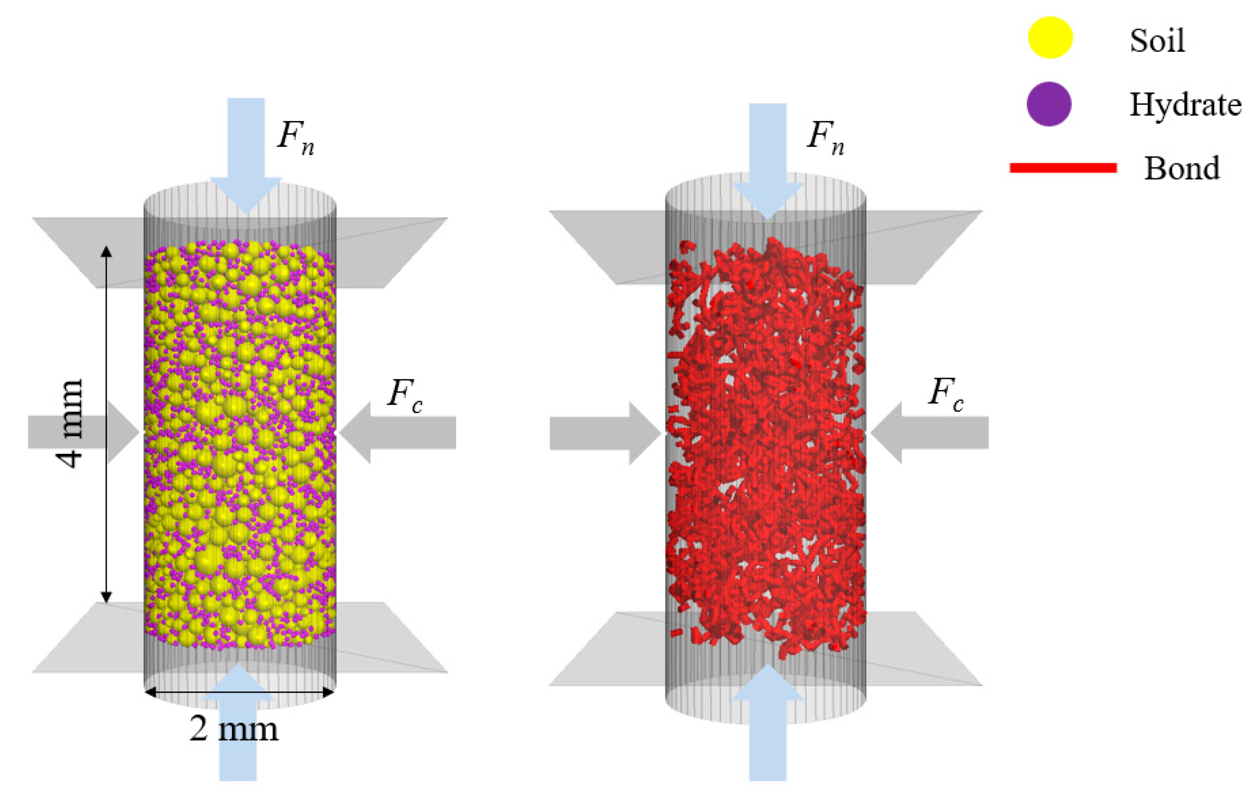
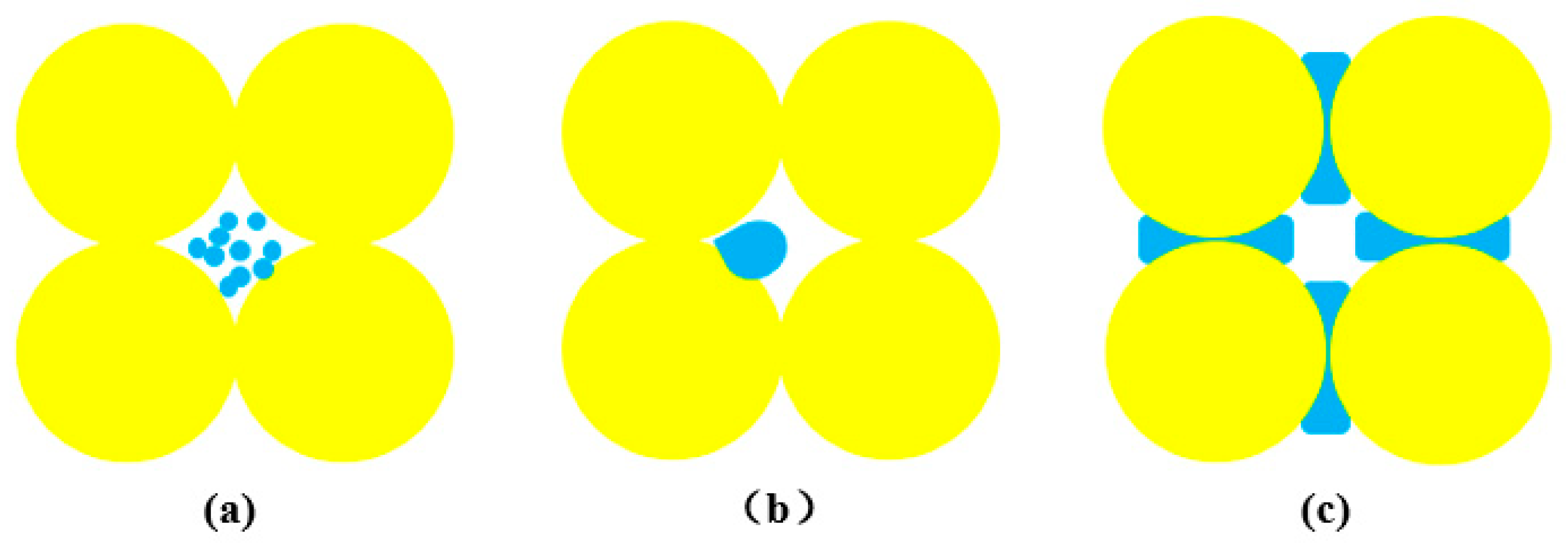
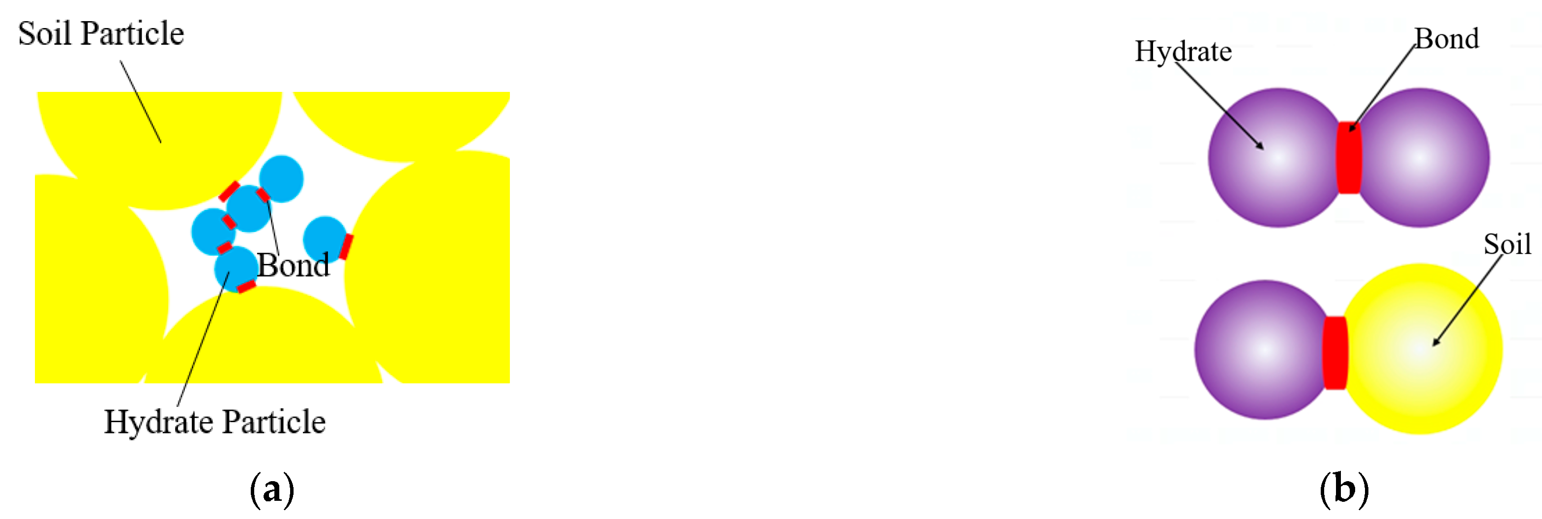
2.1. Model Building

In order to establish a realistic numerical model of hydrate sediment specimens, the particle gradation selected in the model is similar to that of Toyoura sand [26], and the diameter of soil particles is 0.1–0.4 mm. Hydrate particles are generated in the pores of the sediment, and their particle radii are small, while too small a particle radius will inevitably lead to an increase in the number of particles and thus slow down the calculation efficiency. Combining the above factors, the radius of hydrate particles is taken as 0.06 mm. The modeling process is carried out with reference to the modeling method of Cheng [27]. The specific steps are as follows.

(1) Hydrate sediment specimen generation. Firstly, for generating the cylindrical specimen and subsequent loading, three walls were established at the specimen boundary, and then the initial sediment cylindrical specimen with soil particles of 2 mm in diameter and 4 mm in height was generated according to the Toyoura sand grading curve shown in Figure 1, at which time the internal pore ratio of the specimen was 0.42; then, according to the set value range of hydrate particles and soil particles, saturation, and initial porosity, the new porosity and particle size gradation curves were calculated. After that, the sediment cylindrical specimens containing soil particles and hydrate particles were generated according to the particle size gradation curves meeting the requirements of saturation and porosity.

(2) A consolidation pressure F_c was applied to the specimens. A consolidation pressure of 1.0 MPa was applied to the generated specimens so that the particles in the specimens were in contact with each other under this consolidation pressure until the calculation reached equilibrium.

(3) The saturation of specimens was made to reach the desired level. By “cmat” command, a parallel bond model was added between hydrate particles and between hydrate particles and sand particles, and a linear model was added between sand particles to generate a discrete hydrate sediment with 30% saturation, as shown in Figure 2.

(4) Apply loads to the model. The axial load F_n was applied to the model by updating the velocity of the top and bottom walls to ensure that the confining stresses reached the desired stress state [28]. The specimens were tested at a constant loading rate of 1 × 10⁻⁶ m/s under an effective enclosing pressure of 1.0 MPa, and the test was stopped when the axial strain $\epsilon$ reached 25%.

Among them, since the load cannot be applied directly to the wall in the PFC numerical simulation software, servo loading was required according to the difference between the given target load and the actual load applied to the specimen, as shown in Figure 3. The PFC wall velocity conversion equation is [29]:

$$v^w=G({{\displaystyle \sigma }}^{{}^{measured}}-{{\displaystyle \sigma }}^{{}^{required}})=G\Delta \sigma ,$$

(1)

where $\Delta \sigma$ is the difference between the target stress ${{\displaystyle \sigma }}^{required}$ and the actual monitored stress ${{\displaystyle \sigma }}^{measured}$, and G is the servo parameter whose value is calculated using Equation (2) [29]:

$$G=\frac{\alpha A}{{{\displaystyle k}}_n^{{}^{(w)}}{{\displaystyle N}}_c\Delta t},$$

(2)

where α is the stress release factor, taken as 0.5; A is the area of the boundary wall, ${{\displaystyle k}}_n^{(w)}$ is the average contact stiffness, N_c is the number of contacts between the boundary wall and the particles, and $\Delta t$ is the unit time step.

The amount of contact force change caused by the boundary wall motion in the unit time step is [29]:

$$\Delta F^w=k_n{}^{(w)}{N}_c{v}^w\Delta t,$$

(3)

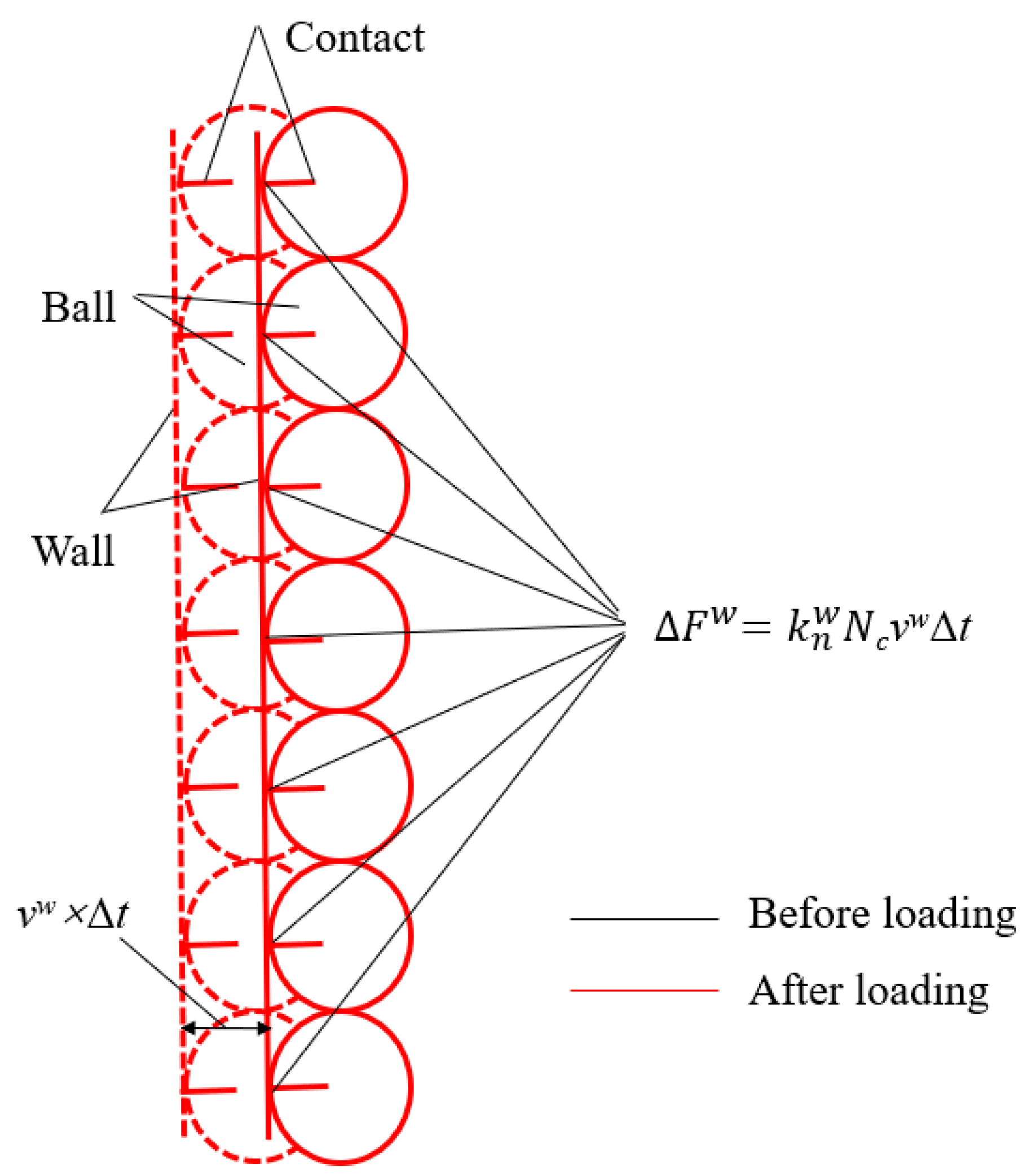
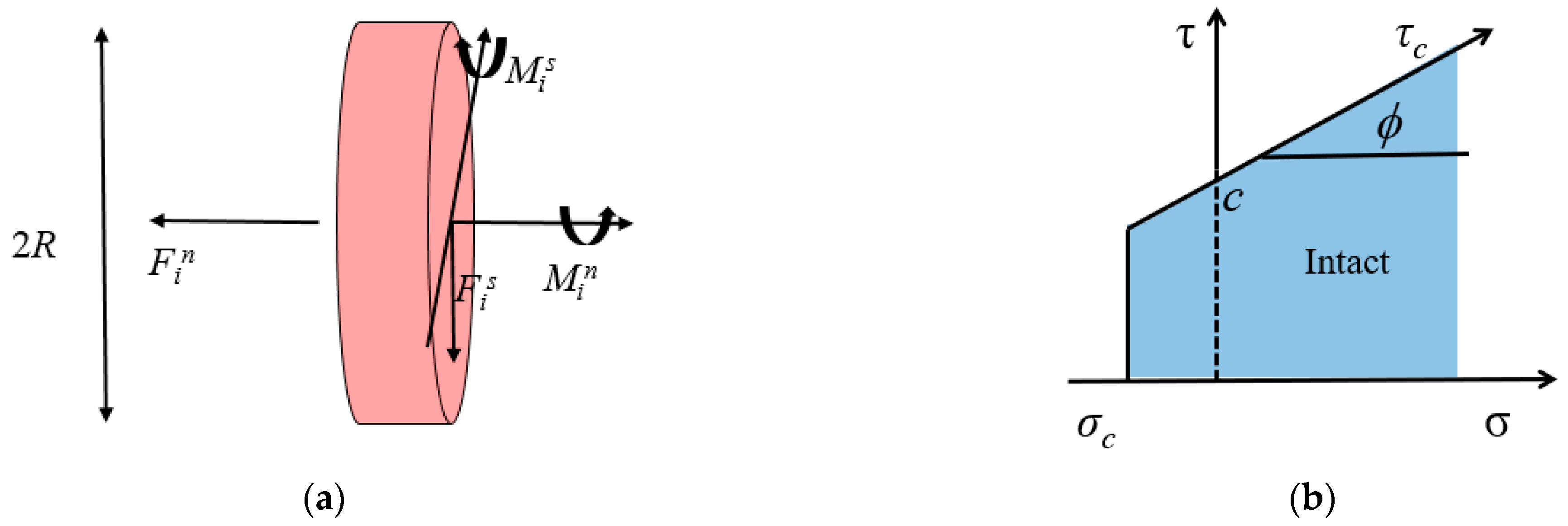
2.2. Contact Models and Parameters

The mechanical properties of hydrate sediments are governed by the hydrate distribution in addition to factors such as net confining pressure, saturation, and mid-major stress coefficient [30]. Hydrate in hydrate sediments exists in three main forms [31], as shown in Figure 3: (i) pore-filling (Figure 4a); (ii) acting as a sediment soil skeleton (Figure 4b), and (iii) cemented between soil particles in the form of colloidal material (Figure 4c). Among them, the results of Waite et al. [32] and Brugada et al. [17] both showed that the pore-filling type has less influence on the mechanical properties of hydrate sediments, and the influence of hydrate distribution factors on the simulation results can be excluded to the maximum extent. Therefore, the pore-filling-type structure is used in the modeling in this paper.

In this paper, the parallel bonding model is chosen to calculate the contact state between particles according to the model of cemented clustered hydrate sediment distribution proposed by Li et al. [31], i.e., there is bonding not only between hydrate and hydrate particles, but also between hydrate and soil particles, as shown in Figure 5. Figure 6a shows the forces and moments transmitted by the cementation. ${{\displaystyle F}}_i$ and ${{\displaystyle M}}_i$ denote the forces and moments acting on the cementation, respectively, which decompose into normal and tangential components along the contact surface [29] (see Equations (4) and (5)). R is the radius of the short cylindrical cementation, and its value is calculated using Equation (6) [33,34]. R⁽¹⁾, and R⁽²⁾ are the radii of the two spheres at contact. $\lambda$ is a dimensionless parameter, and if $\lambda$ is 1, the cemented material will fill the particles in contact with each other as much as possible.

$${{\displaystyle F}}_i={{\displaystyle F}}_i^n+{{\displaystyle F}}_i^s,$$

(4)

$$M_i=M_i^n+M_i^s,$$

(5)

$$R=\lambda min(R^{(1)}, R^{(2)}),$$

(6)

The parallel bonding model is defined by five parameters: normal stiffness k_n, tangential stiffness k_s, normal strength tangential strength ${{\displaystyle \tau }}_c$, and short cylindrical radius R of the cementation. The maximum normal ${{\displaystyle \sigma }}^{max}$ and tangential stresses ${{\displaystyle \tau }}^{max}$ can be expressed as [35]:

$${{\displaystyle \sigma }}^{{}^{max}}=\frac{{{\displaystyle -F}}^{{}^n}}{A}+\frac{\left|{{\displaystyle M}}^{{}^s}\right|R}{I},$$

(7)

$${{\displaystyle \tau }}^{{}^{max}}=\frac{\left|{{\displaystyle F}}^{{}^s}\right|}{A}+\frac{\left|{{\displaystyle M}}^{{}_{}^n}\right|R}{I},$$

(8)

where A, I, and J are cross-sectional area, cross-sectional moments of inertia, and cross-sectional polar moments of inertia, respectively, using the following calculation formulas: A = πR², I = 0.5πR⁴ and J = 0.25πR⁴.

As shown in Figure 6b, if the maximum normal stress exceeds its tensile strength limit (${{\displaystyle \sigma }}^{max}$ ≥ ${{\displaystyle \sigma }}_c$), or the maximum tangential stress exceeds the shear strength limit (${{\displaystyle \tau }}^{max}$ ≥ ${{\displaystyle \tau }}_c$), the parallel bonding model will be destroyed.

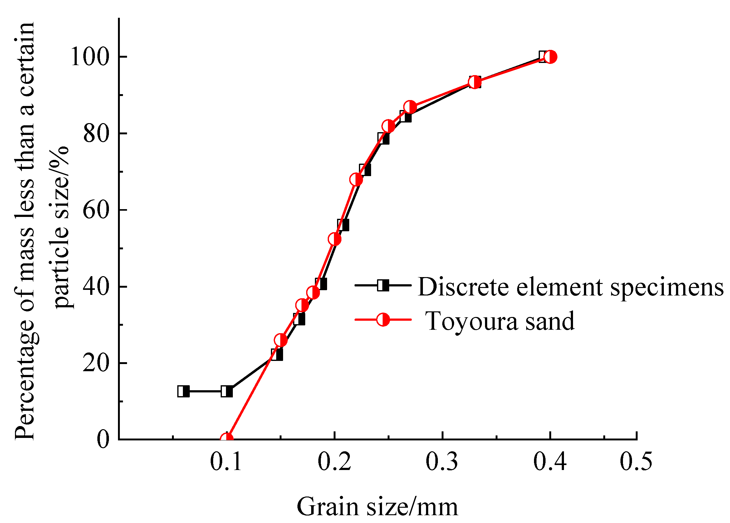
2.3. Model Validation

In order to determine the meso parameters of the numerical model in this paper, the simulation results of Brugada et al. [17] were used as the basis for calibration, and the trial and error method was used to continuously and dynamically adjust the meso parameters until the curves in this paper basically matched with the curve of Brugada et al. The final calibration results are shown in Figure 7, and the meso parameters determined after calibration are shown in

Table 1. Material parameters in discrete element simulation.

Type	Density/(g/cm3)	Friction Coefficient	Linear Model		Gluing Model
			Effective Modulus/(MPa)	Stiffness Ratio	Effective Modulus/(MPa)	Stiffness Ratio	Tensile Strength/(MPa)	Bond Strength/(MPa)	Friction Angle/(°)
Soil particles Hydrate particles	2.3	0.75	286	1.43
Between hydrate particles	0.9	0.75	28.6	1.43	24	1.5	5	5	40
Between hydrate particles and soil particles					24.6	1.5	5	5	40

. It can be seen that the trends of the two sets of curves are generally consistent and can be roughly divided into three stages. The first stage is the linear elastic stage, where the bias stress of the sediment specimen increases approximately linearly with the increase in axial strain; the second stage is the yield stage, where the bias stress reaches its peak. The peak strength of the bias stress simulated in this paper is 1.52 MPa, and that of Brugada et al. is 1.54 MPa, with an error of only 1.3% between them; the third stage is the residual stage, where both sets of simulations show strain softening and the bias stress rapidly decreases and tends to a stable value, and the specimen is damaged. The second half of the curve derived in this paper has a certain degree of jitter, which is because, in the compression process, a small displacement or misalignment of the particles will cause a relatively obvious change in the stress monitored on the monitoring wall with the increase in particle density. In general, the numerical simulation curve results in this paper have good accuracy.

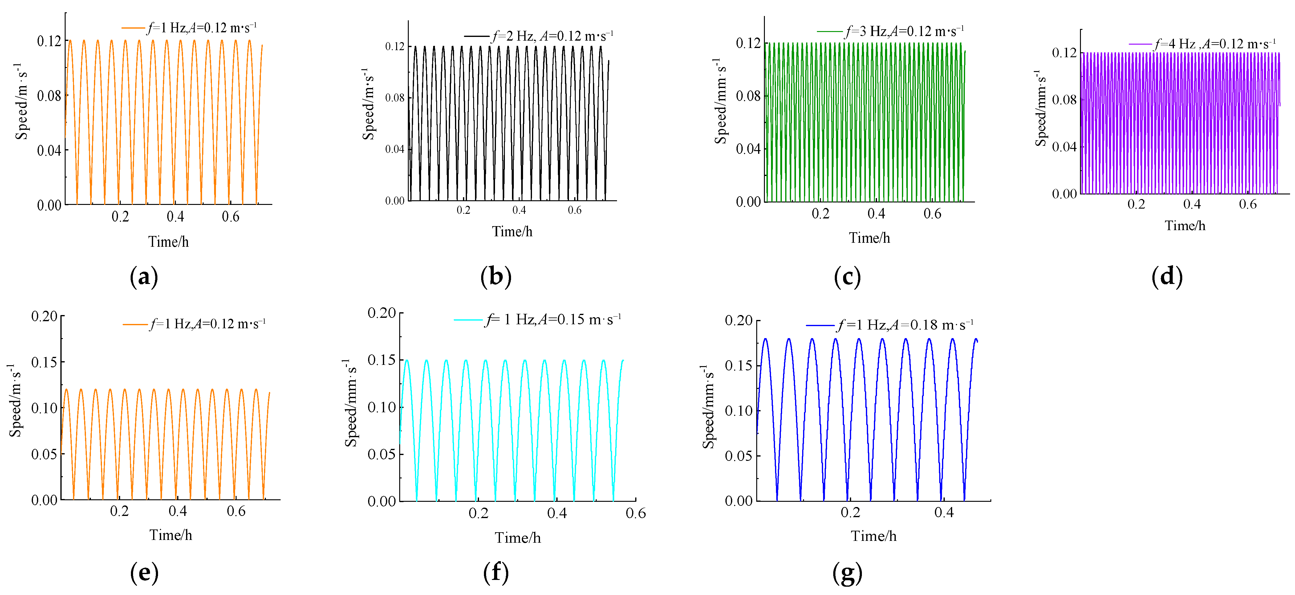
2.4. Simulation Scheme

At present, displacement-controlled loading is commonly used in tests or simulations to equate the vibrational loading of earthquakes, i.e., the velocity magnitude is kept constant during the loading process, and the loading and unloading are added and removed back and forth within a certain displacement range [35,36,37], but this is not consistent with reality, and the velocity of real seismic waves changes continuously with time. Therefore, in order to reveal the macro-meso structural evolution of hydrate sediments under dynamic loading and its mechanical properties, this paper simulates dynamic loading by varying the axial loading velocity. In general, a seismic wave is a kind of random wave, and the random wave can be described by its amplitude, period, and phase. Although discrete elements can simulate random waveforms, the interpretation of the dynamic response mechanism of hydrate sediments under the action of random waveforms is very complicated. For this reason, the regular sinusoidal wave loading velocity will be introduced for analysis in this paper, and its expression is

$$v^w=A\sin (2\mathsf{\pi }f\ast t),$$

(9)

where $A$ is the loading amplitude, $f$ is the loading frequency, and $t$ is the time.

Since the frequency of seismic waves is generally less than 10 Hz, four frequencies of f = 1, 2, 3, and 4 Hz were selected in this paper. Three amplitudes of A = 1.2 × 10⁻¹, 1.5 × 10⁻¹, and 1.8 × 10⁻¹ m·s⁻¹ were selected based on the peak wave velocity recorded in Hachinohe, Japan [38], according to which different cyclic loading schemes were composed, as shown in

Table 2. Simulation scheme.

Title	Frequency/Hz	Peak/m·s−1
Sine wave	1, 2, 3, 4	1.2 × 10−1
Sine wave	1.0	1.2 × 10−1, 1.5 × 10−1, 1.8 × 10−1

. The adopted cyclic velocity curves are shown in Figure 8.

3. Results and Analysis

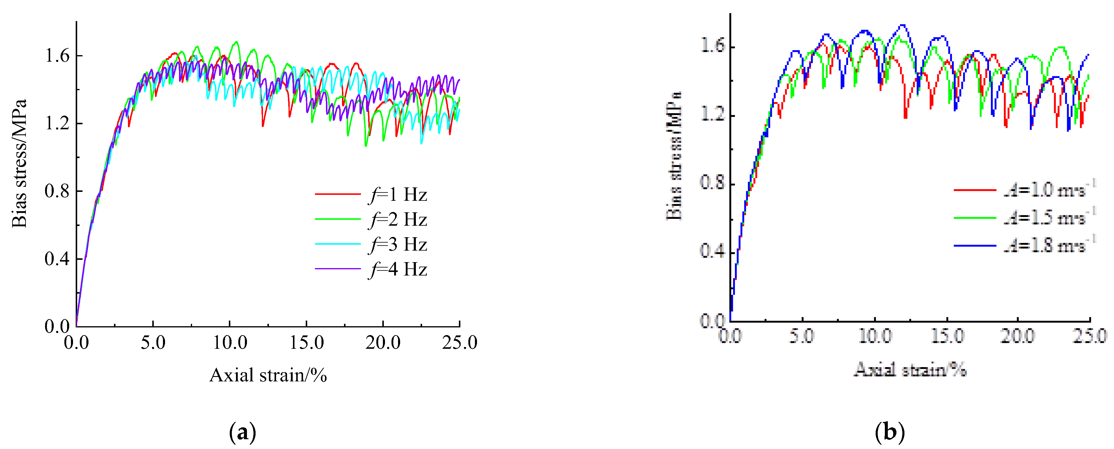
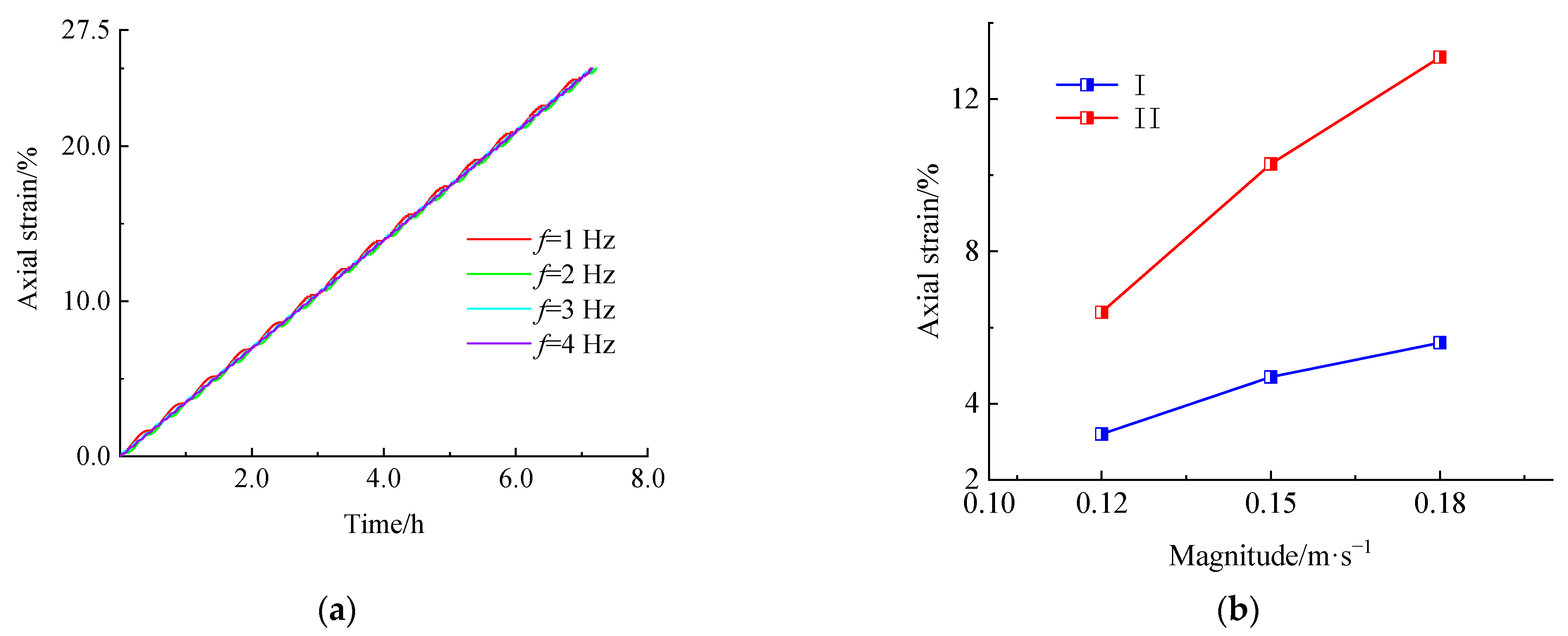
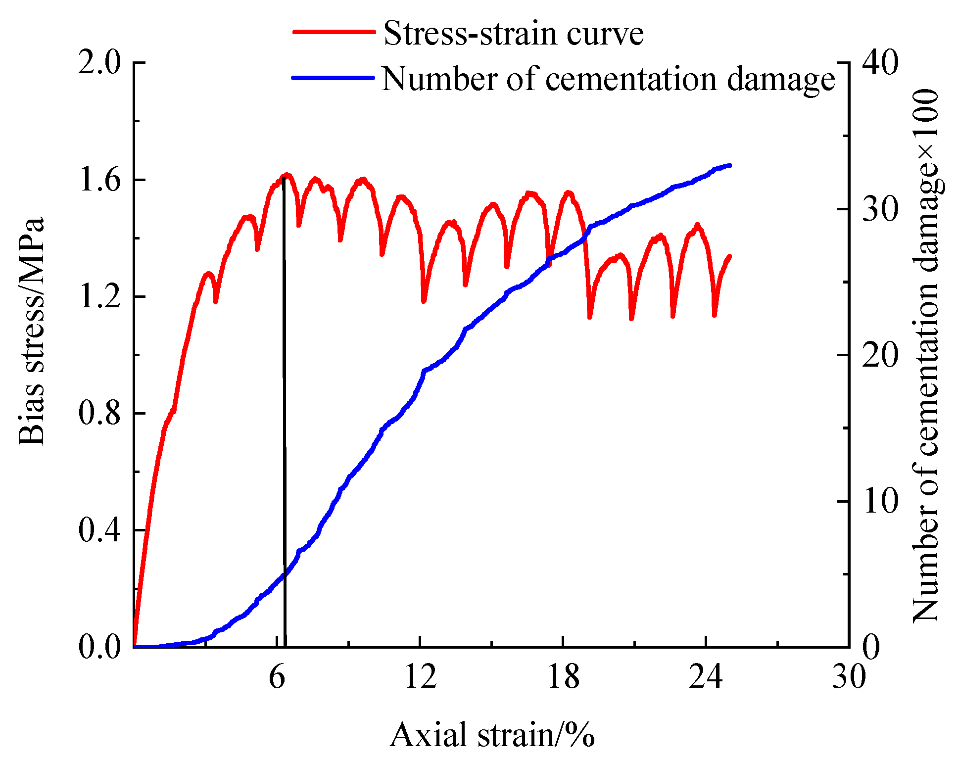
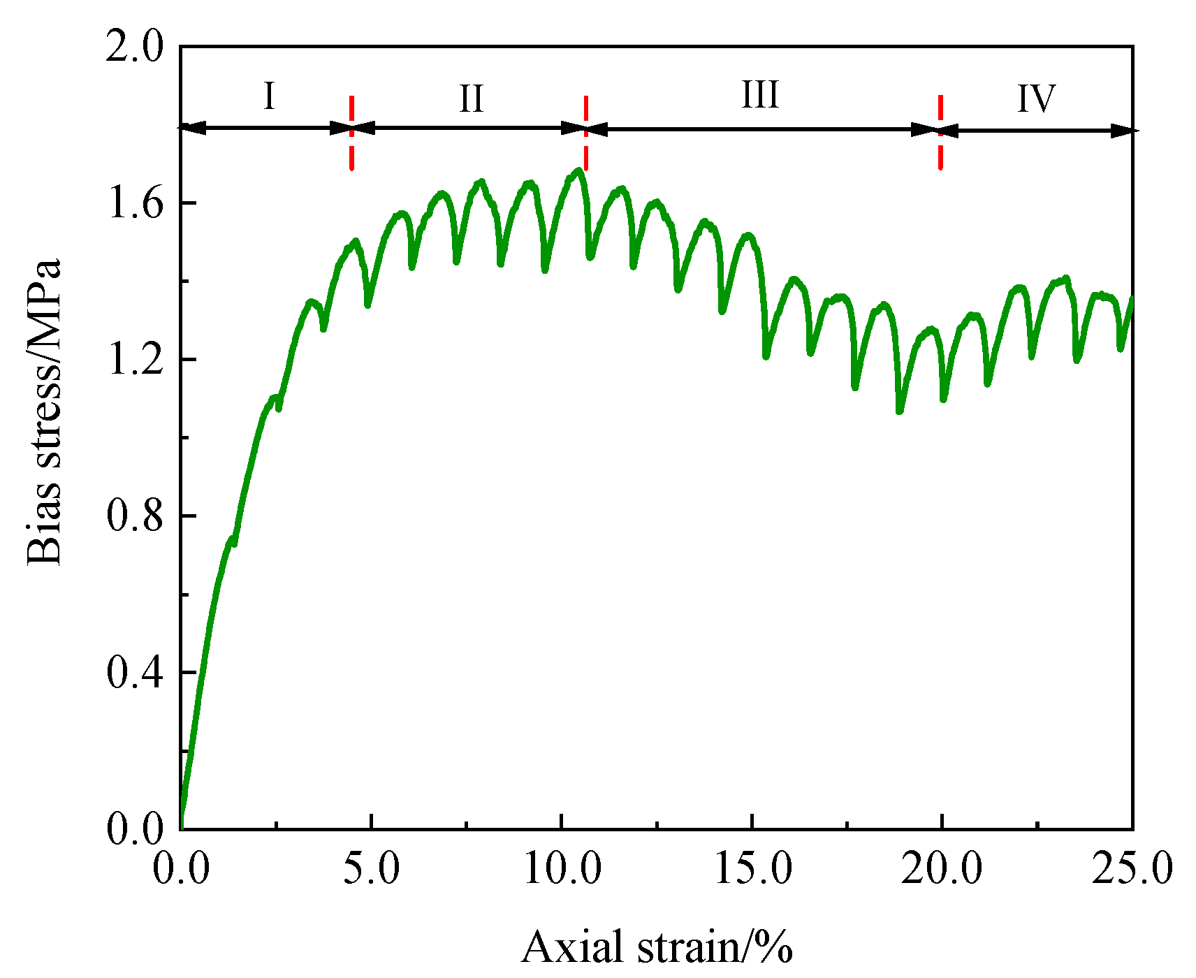
3.1. Stress–Strain Curves

Unlike quasi-static loading, the mechanical characteristics of hydrate sediments under dynamic loading conditions change continuously with the cyclic change of loading velocity. To analyze the mechanical characteristics of hydrate sediment under dynamic loading, the stress–strain of hydrate sediment under dynamic loading of f = 2 Hz and A = 0.12 m s⁻¹ as shown in Figure 9 was analyzed as an example. It can be seen that the stress–strain curves of hydrate sediment under dynamic loading can be roughly divided into four stages. The first stage is the elastic stage, which obeys Hooke’s law and shows the elastic characteristics, and the stress–strain curve is a straight line with a fixed slope. With the increase in axial strain, the slope of the curve slowly decreases, and the specimen enters the second stage (yield stage), in which the slope decreases continuously before the curve reaches the peak point, and the stress increases nonlinearly with strain and increases slowly. During this stage, the sediment specimen is compressed, the skeleton and cementation are destroyed, and the particles are rearranged. At the same time, the pores within the sediment specimen are squeezed under pressure, which makes the volume of the specimen decrease, at which time the bearing capacity of the specimen decreases, and thus the elastic modulus of the specimen gradually decreases. The third stage is the strain softening stage. After the peak point of the stress–strain curve, the partial stress decreases with the increase in the axial strain. The strength of the hydrate sediment specimen starts to decline slowly, and the stress–strain curve shows a strain softening trend. The fourth stage is the strain strengthening stage. In this stage, the partial stress increases with the increase in axial strain, which is because the hydrate particles in the sediment specimen still have a certain cementing effect on them, which can resist part of the stress. At the same time, the interaction between the particles caused by the presence of the surrounding pressure increases the contact area and frictional resistance, which inhibits the increase in cracks and prevents the slip or rearrangement between the particles, making the specimen more resistant to the damage caused by the axial load. As the loading proceeds, the particles inside the specimen are rearranged, the specimen is slowly and fully stressed, and its load-bearing capacity is gradually stabilized so that the sample also maintains a certain strength.

The stress–strain curves of hydrate sediment under different loading frequencies and different loading amplitudes are shown in Figure 10. As can be seen from the figure, the stress–strain curve of the velocity cyclic loading mode is different from the force cyclic loading mode, and its stress–strain curve does not form a closed hysteresis loop curve, which is because even though the loading speed decreases, the axial displacement in the simulation keeps increasing downward, i.e., the hydrate sediment specimen keeps loading state without the process of unloading in the force cyclic loading mode.

It can also be seen from the figure that the change in the frequency and amplitude of the loading rate will have some effect on the characteristics of the stress–strain curve of the hydrate sediment. For this reason, the relationship between the axial strain interval L of the sediment and the loading conditions (Stages I and II) was counted, as shown in Figure 11. As can be seen from the figure, the axial strain corresponding to Stage I under all loading frequency conditions is 3.2%, which means that the loading frequency does not affect the distribution range of hydrate sediment specimens in Stage I. However, with the increase in the loading amplitude, the L corresponding to the first stage also increases, and when the loading amplitude increases from 0.12 m s⁻¹ to 0.18 m s⁻¹, the L corresponding to the first stage is, respectively, 3.2%, 4.7%, and 5.6%. It shows that as the loading amplitude increases, the L corresponding to the elastic phase of the specimen becomes shorter, which is since the strength limit of the specimen is certain, and the greater the dynamic loading action, the faster it reaches its elastic limit.

In Stage II, as the loading frequency increases, the L corresponding to the yielding stage of the specimen first increases and then decreases; when the loading frequency increases from 1 Hz to 2 Hz, the L corresponding to Stage II are, respectively, 6.4% and 9.1%. This is because the higher the loading frequency, the shorter the loading cycle, i.e., the shorter the action time of each cycle, the less the cementation damage inside the specimen. However, as the loading frequency continues to increase from 2 Hz to 4 Hz, the L corresponding to phase II is 9.1%, 7.3%, and 6.4%, respectively. This is due to the fact that the more the number of cycles of cyclic loading at the same time, the collodion damage inside the specimen increases, making the time experienced in the yielding phase of the specimen decrease with the change in frequency. As the loading amplitude increases, the L corresponding to the yielding stage of the specimen also increases. When the loading amplitude increases from 0.12 m·s⁻¹ to 0.18 m·s⁻¹, the L corresponding to the second stage is, respectively, 6.4%, 10.3%, and 13.1%. This is because the larger loading amplitude indicates that the specimen is loaded at a larger rate in the same cycle, i.e., the larger the axial force on the specimen in each cycle, the larger the load carrying capacity of the specimen, which is also in accordance with the characteristics of the hydrate sediment as a frictional material.

Figure 12 shows the strain–time curves of hydrate sediments under different dynamic loads. It can be seen that the strain–time curves vary basically the same for different loading frequencies, but the strain rate increases with the increase in loading amplitude. It shows that the loading amplitude has a greater effect on the strain of hydrate specimens. This is due to the fact that the larger the loading amplitude is at the same loading frequency, the greater the stress on the specimen in each cycle, the greater the number of cementation damage, the easier the specimen is to deform and destroy, and the greater the strain rate.

3.2. Strength Characteristics

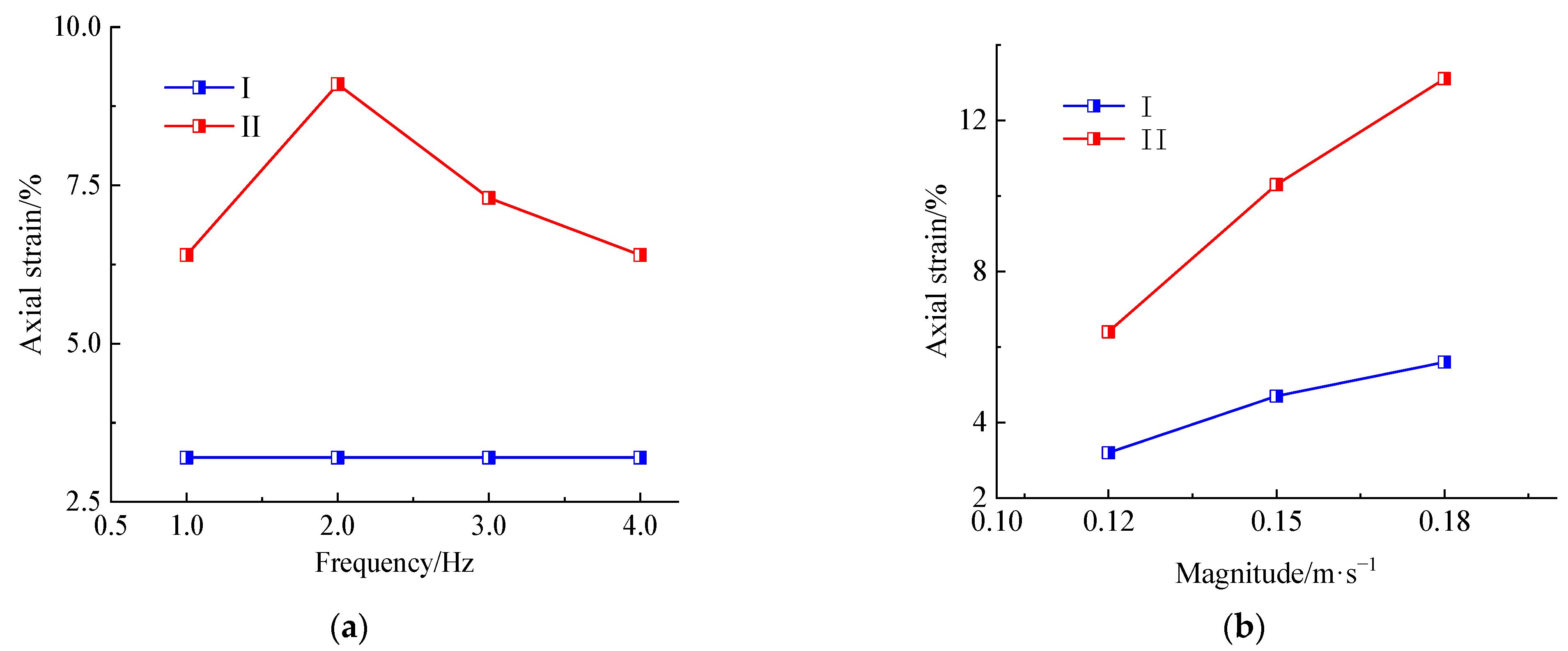
3.2.1. The Effect of Loading Frequency

Figure 13 shows the relationship between the peak sediment strength, the sediment E₅₀, and the loading frequency. From the figure, it can be seen that the peak sediment strength increases and then decreases as the loading frequency increases. When the loading frequency increases from 1 Hz to 2 Hz, the peak sediment strength increases from 1.62 MPa to 1.68 MPa, and its peak strength increases by 3.7% compared to 1 Hz. When the loading frequency continues to increase to 3 Hz and 4 Hz, the peak sediment strength decreases to 1.6 MPa and 1.59 MPa, respectively, and decreases by 5% and 5.2% compared to 2 Hz, respectively. It shows that the effect of loading frequency on the peak strength is not monotonic, and there exists a critical value, less than which the peak strength increases with increasing loading frequency, and greater than which the peak strength decreases with increasing loading frequency. This is due to the loading frequency being small, as the loading cycle becomes shorter with the increase in loading frequency. That is, the shorter the time of the action of each cycle with the same number of cycles, the specimen’s internal cementation damage is less, and the bearing capacity of the specimen is greater. However, as the loading frequency continues to increase beyond its critical value, the number of cyclic loading at the same time increases, and the cementation damage inside the specimen increases. Comparing the length of the action time of each cycle, the influence of the number of cyclic loading within the same time on the cementation damage dominates, which makes the bearing capacity of the specimen decrease. At the same time, when the loading frequency exceeds the critical value, the particles inside the sediment specimen frequently adjust the arrangement, which leads to the instability of the internal mechanical structure of the sediment and makes the internal force uneven, and even generates the stress concentration phenomenon, and finally leads to a certain degree of reduction in the yield strength of the sediment specimen.

Hydrate sediments are inelastic materials, so it is difficult to obtain the initial modulus E₀. In this test, the cut-line modulus E₅₀ was used to describe the stiffness of the specimen. E₅₀ is defined as the slope of the line connecting the point half the value of the breaking strength in the stress–strain curve to the origin. From the relationship between the sediment E₅₀ and the loading frequency in Figure 13, it can be seen that the E₅₀ of the sediment specimen is 0.58 MPa at a loading frequency of 1 Hz, 0.57 MPa when the loading frequency increases to 2 Hz, 0.56 MPa when the loading frequency continues to increase to 3 Hz, and 0.57 MPa when the loading frequency continues to increase to 4 Hz. With the increase in loading frequency, the E₅₀ of hydrate specimens changed less, only 0.01 MPa, which means that the effect of loading frequency on the stiffness of hydrate specimens is small.

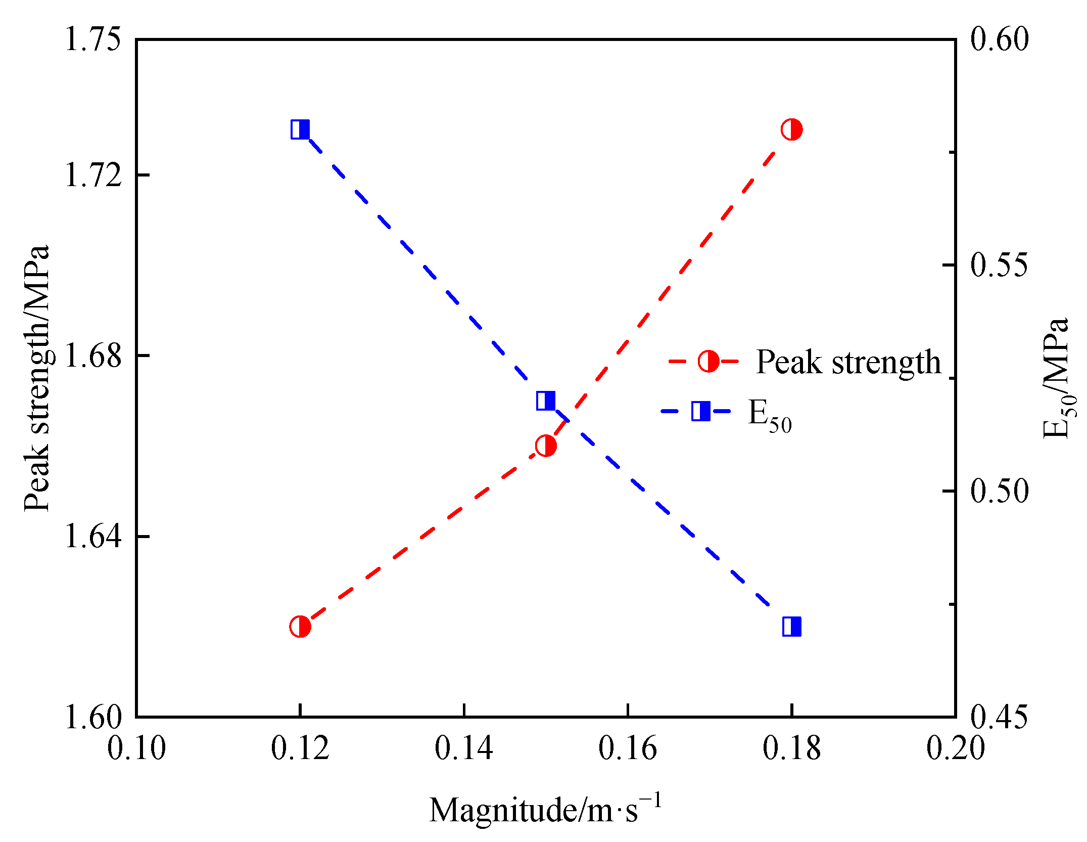
3.2.2. The Effect of Loading Amplitude

Figure 14 shows the curve of peak sediment strength, sediment E_50, and loading amplitude. When the loading amplitude was increased from 0.12 m s⁻¹ to 0.18 m s⁻¹, the peak sediment strengths were 1.62 MPa, 1.66 MPa, and 1.73 MPa, respectively, which were 2.4% and 6.7% higher compared to the peak strengths at loading frequencies of 0.15 m·s⁻¹ and 0.18 m·s⁻¹ for a loading amplitude of 0.12 m·s⁻¹, respectively. Under the action of loading, the particles in the sediment specimen will first overcome the interparticle interaction forces before the relative misalignment occurs, mainly including interparticle friction and cohesion. When the amplitude of the loading rate increases, due to the inertia of the sediment particles, particle-to-particle squeezing begins to occur, resulting in an increase in the positive stress between the sediment particles, which in turn increases the inter-particle friction and the strength of the sediment. Combined with Figure 12b, the strain rate of the specimen increases with the increase in loading amplitude under dynamic loading, and the time required for the specimen to respond to strain decreases with the increase in strain rate. This makes the strain more localized, and then makes the specimen all strained and will require more stress so the peak strength of the specimen will increase as the cyclic loading amplitude increases.

The relationship between the E₅₀ loading amplitude of the sediment in Figure 14 shows that the E₅₀ of the hydrate specimen decreases with the increase in the loading amplitude. The E₅₀ of the sediment specimen was 0.58 MPa at a loading amplitude of 0.12 m s⁻¹; when the loading amplitude increased to 0.15 m s⁻¹, the E₅₀ decreased to 0.52 MPa with a decrease of 10.3%; when the loading amplitude continued to increase to 0.18 m s⁻¹, the E₅₀ decreased again to 0.47 MPa with a decrease of 9.6%. This is due to the fact that the cementation between soil and hydrate particles in the sediment specimen will be destroyed under the action of loading, and the rearrangement between the particles will occur; the greater the loading amplitude, the greater the stress on the specimen in each cycle, and the greater the number of cementation failures, which makes the sediment specimen less able to resist deformation and reduces the stiffness of the specimen.

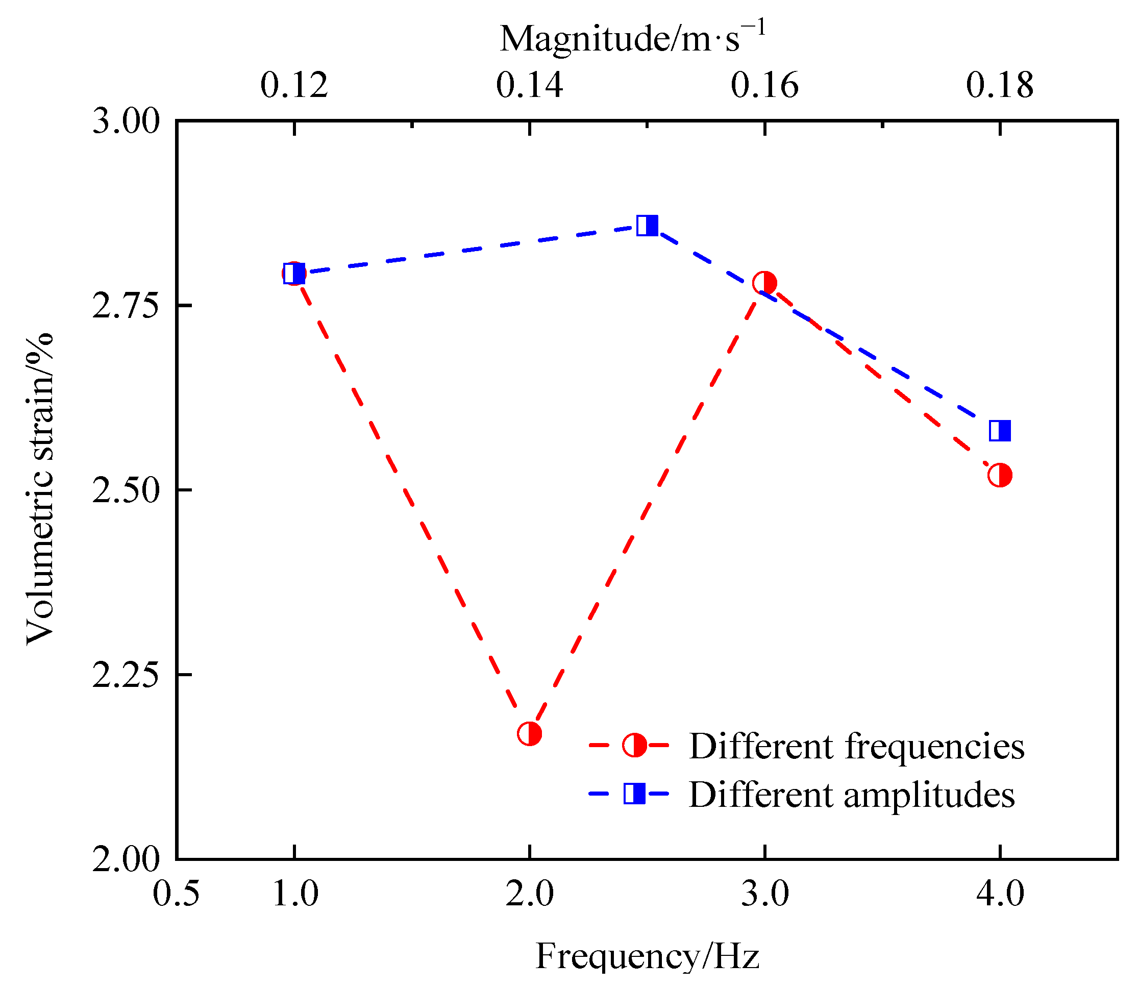
3.3. Volumetric Strain Characteristics

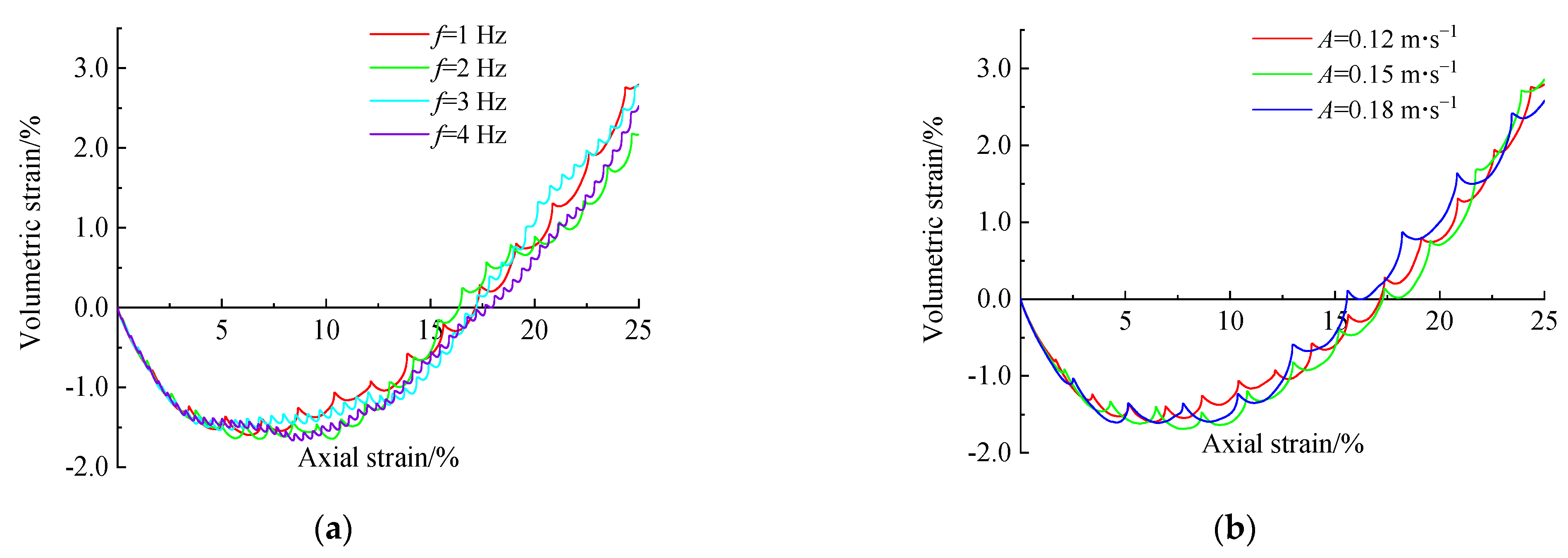
3.3.1. Comparison of Volume Strain Curves

Dilatancy is one of the most important properties of sandy soils. This is because most of the accidents under load are due to shear swell or shear shrinkage damage of the soil, which leads to the loss of bearing capacity. Hydrate sediments have a similar structure to sandy soils, so their dilatancy is important to study [39]. The results of volume strain simulations of hydrate sediments under different dynamic loads are shown in Figure 15. It can be seen that the simulation results of each group show the bulk strain law of shear shrinkage followed by shear dilatancy. Firstly, as the loading proceeds, the pore ratio between the specimen particles decreases with the increase in consolidation pressure, which makes the specimen appear to have obvious shear shrinkage. Then, as the loading continues, the cementation in the specimen gradually breaks down, and because the soil particles are closely arranged, the soil particles at the shear zone must rotate around the adjacent particles in order to produce larger movement, which causes the expansion of the specimen. It can also be seen from the figure that the correlation between the shear shrinkage of hydrate sediment and the loading frequency and amplitude is small. However, the maximum shear dilatancy is influenced by the loading frequency and loading amplitude.

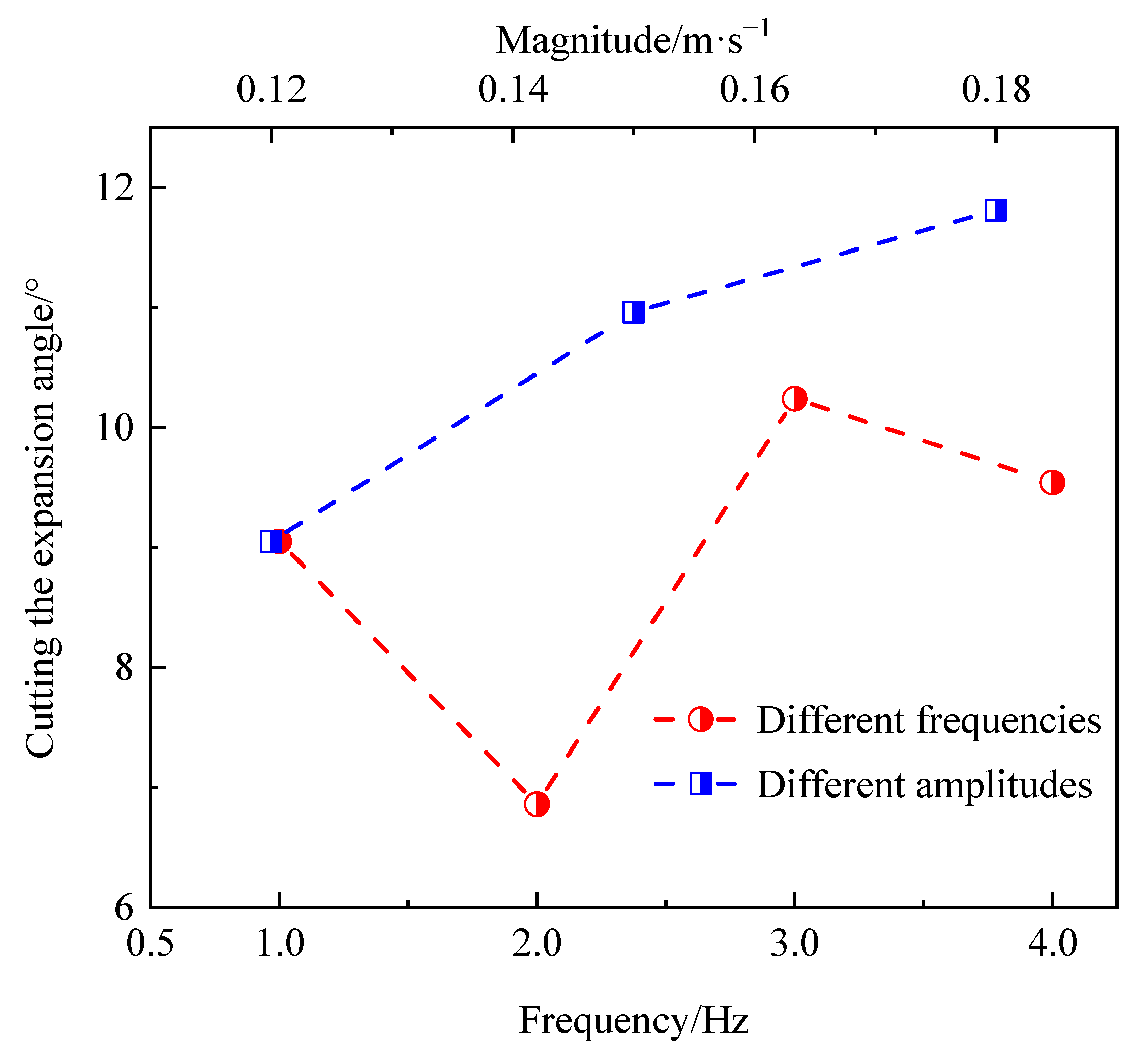
3.3.2. Frequency, Amplitude–Dilation Relationship

To quantify the effects of loading frequency and loading amplitude on shear dilatancy, the maximum shear dilatancy under different loading frequencies and loading amplitude conditions were counted separately, as shown in Figure 16. It is obvious from the figure that the maximum shear expansion of sediment specimens at loading frequencies of 1, 2, 3, and 4 Hz are 2.793%, 2.17%, 2.780%, and 2.52%, respectively, which means that the shear dilatancy decreases and then increases and finally decreases again with the increase in frequency. At the loading amplitudes of 0.12, 0.15, and 0.18 m s⁻¹, the maximum shear dilatancy was 2.79%, 2.858%, and 2.52%, respectively, which also increased and then decreased with increasing amplitude. As Figure 15 shows, it can be seen that there is a critical point between shear shrinkage and shear dilatancy of the specimen, called the phase change point. The more forward the phase change point is, the shorter the shear shrinkage process is and the more obvious the shear expansion of the specimen is. At a frequency of 2 Hz, the phase change point is the most forward compared to the other three groups, and the maximum shear dilatancy of the specimen is the smallest at 2.17%. This is because the specimen with an axial strain of about 25% at a frequency of 2 Hz is exactly in the process of a certain increase in the load-bearing capacity after the rearrangement of the particles, resulting in a consequent decrease in its maximum shear expansion.

As can be seen from Figure 16, the effect of loading amplitude on shear dilatancy amount is not monotonic as the loading amplitude increases. The maximum shear dilatancy of the sediment specimens increased with increasing amplitude at the loading amplitude of 0.12, 0.15 m s⁻¹, 2.79%, and 2.858%, respectively. At the amplitude of 0.18 m s⁻¹, the phase change point was the most forward compared to the other three groups, while the maximum shear dilatancy of the specimens was the smallest at 2.52% for the same reason as described in the previous paper.

The variation of the shear dilatancy angle with different loading frequencies and amplitudes are given in Figure 17. The formula for the shear dilatancy angle $\psi$ proposed by Roscoe [40] is as follows.

$$\psi =\arcsin -\frac{{{\displaystyle \epsilon }}_{{}_1}+{{\displaystyle \epsilon }}_{{}_2}}{{{\displaystyle \epsilon }}_{{}_1}-{{\displaystyle \epsilon }}_{{}_2}},$$

(10)

where ${\epsilon }_1$ and ${\epsilon }_2$ are the axial and lateral strain increments, respectively.

As can be seen from Figure 17, the variation law of shear dilatancy angle of sediment specimens with loading frequency under the action of the same loading amplitude is similar to the variation law of shear dilatancy amount with loading frequency, and the shear dilatancy angle of specimens under the action of the same loading frequency tends to increase linearly with the increase in loading amplitude. It was shown [41] that when the shear dilatancy angle was higher, the sediment specimens obtained larger lateral deformation, and the precursors of instability damage of the specimens were more obvious. That means that the higher the loading frequency of the test conditions, the more likely the sediment specimens are to have destabilization damage.

3.4. Volumetric Strain Characteristics

Under a triaxial stress state, hydrate sediments exhibit their deformation damage process in terms of stress–strain and bulk strain development changes at the macroscopic level and shear zone generation and development at the fine level [42]. The effect of loading frequency and amplitude on the deformation damage of hydrate sediment specimens can be studied by particle displacement, contact force chain distribution, and microcrack extension evolution law.

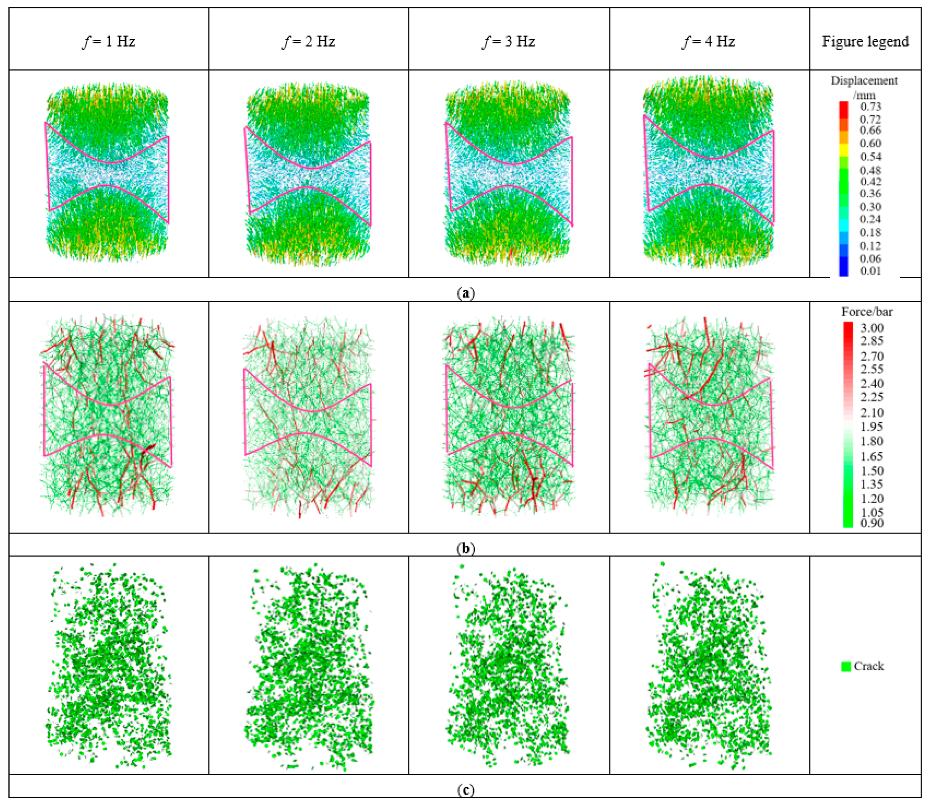
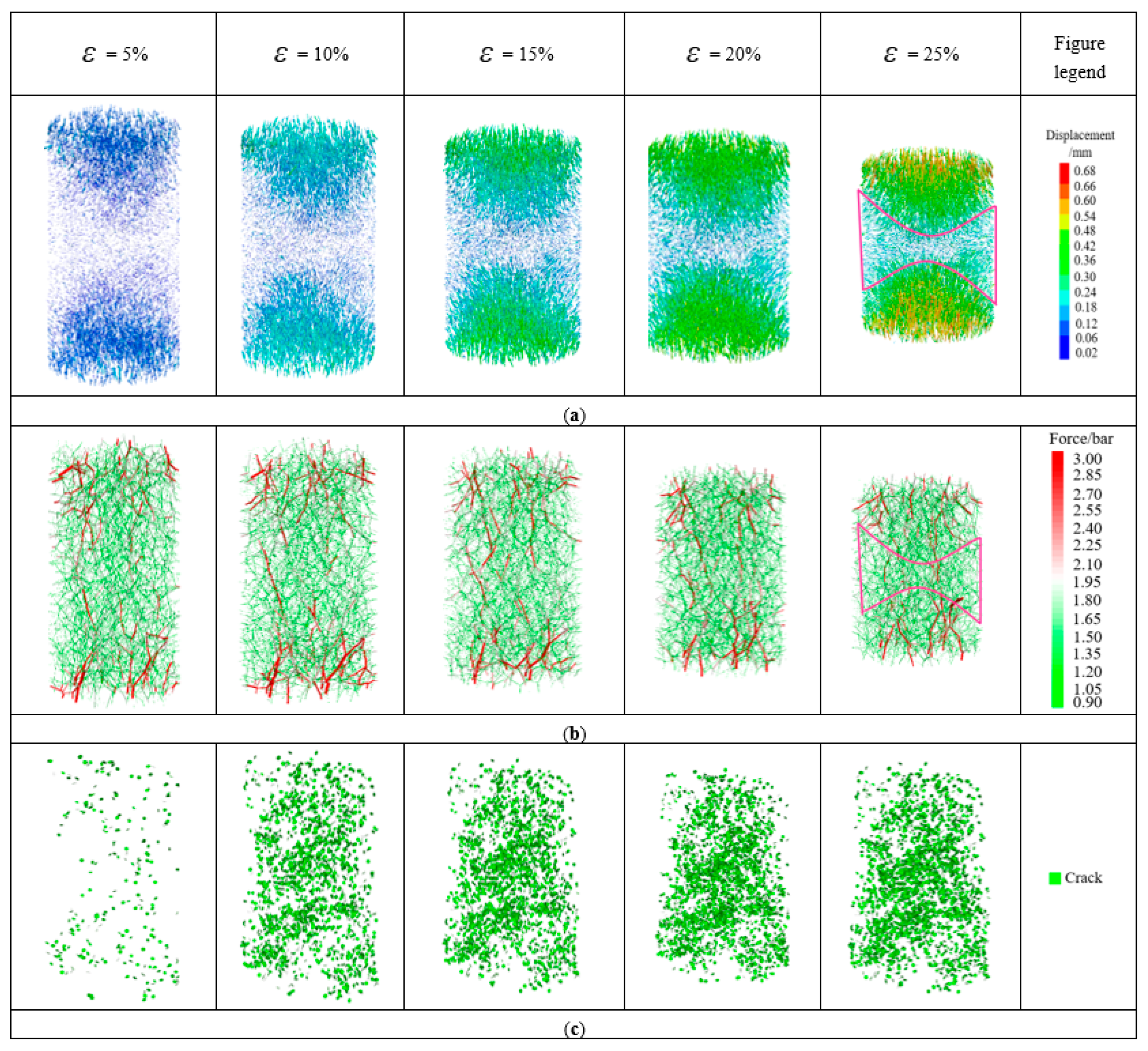
3.4.1. Evolution of Deformation and Failure Characteristics

Taking the deformation damage law of hydrate sediment under f = 1.0 Hz, A = 0.12 m·s⁻¹ dynamic load as an example, the particle displacement, contact force chain distribution, and microcrack expansion simulation results are shown in Figure 18. From the particle displacement cloud shown in Figure 18a, it can be seen that with the increase in axial strain, the particles in the upper and lower parts of the model are compressed and move toward the middle, and the pores inside the model are gradually compressed and form a shear zone, as shown in the area marked by the black wire frame in the figure. From the contact force chain cloud shown in Figure 18b, it can be seen that a weak force chain (green part) is formed at the center of the shear zone, the strong force chain (red part) gradually expands toward the ends of the shear zone of the specimen, and the contact force near the shear zone is roughly perpendicular to the particle displacement direction, which corresponds to the displacement cloud atlas of the particles. This is due to the frictional forces generated by the misalignment of the particles in the specimen, which are composed of unbalanced forces between the particles when relative sliding is generated by the particles inside the specimen [43].

From the microcrack expansion diagram shown in Figure 18c, it can be seen that the number of cracks at 5% of axial strain (before the peak strength) is small and mainly concentrated at the two ends of the specimen, and there is no obvious cementation damage in the hydrate sediment specimen. The number of cracks increases significantly at 10% and 15% of the axial strain (after the peak strength). At this time, the cementation between the hydrate particles and the cementation between the hydrate particles and the soil particles are destroyed in large quantities, but the cracks are randomly distributed in an irregular manner. The number of cracks in the specimen tends to be stable at 20% and 25% of the axial strain (after shear expansion), so it can be seen that the change law of the number of cracks in the specimen with the axial strain is similar to the change law of the stress–strain relationship. The number of cracks in the middle of the specimen is significantly larger than the number of cracks at the two ends of the specimen, which indicates that the number of collodion damage near the shear zone continues to increase with the further increase in the axial strain and is concentrated near the shear zone.

A similar conclusion can be drawn from the damage–strain relationship curve of stress–cementation in Figure 19. The degree of stress is low in the initial stage of specimen loading, the cementation damage is less, and the rate of cementation damage is slow. With the development of strain reaching the peak strength, the rate of cementation damage increases significantly, and the cementation damage increases by a large amount; thus, the development of cementation damage can explain to some extent the process of change in the macroscopic mechanical behavior of the specimen during the test.

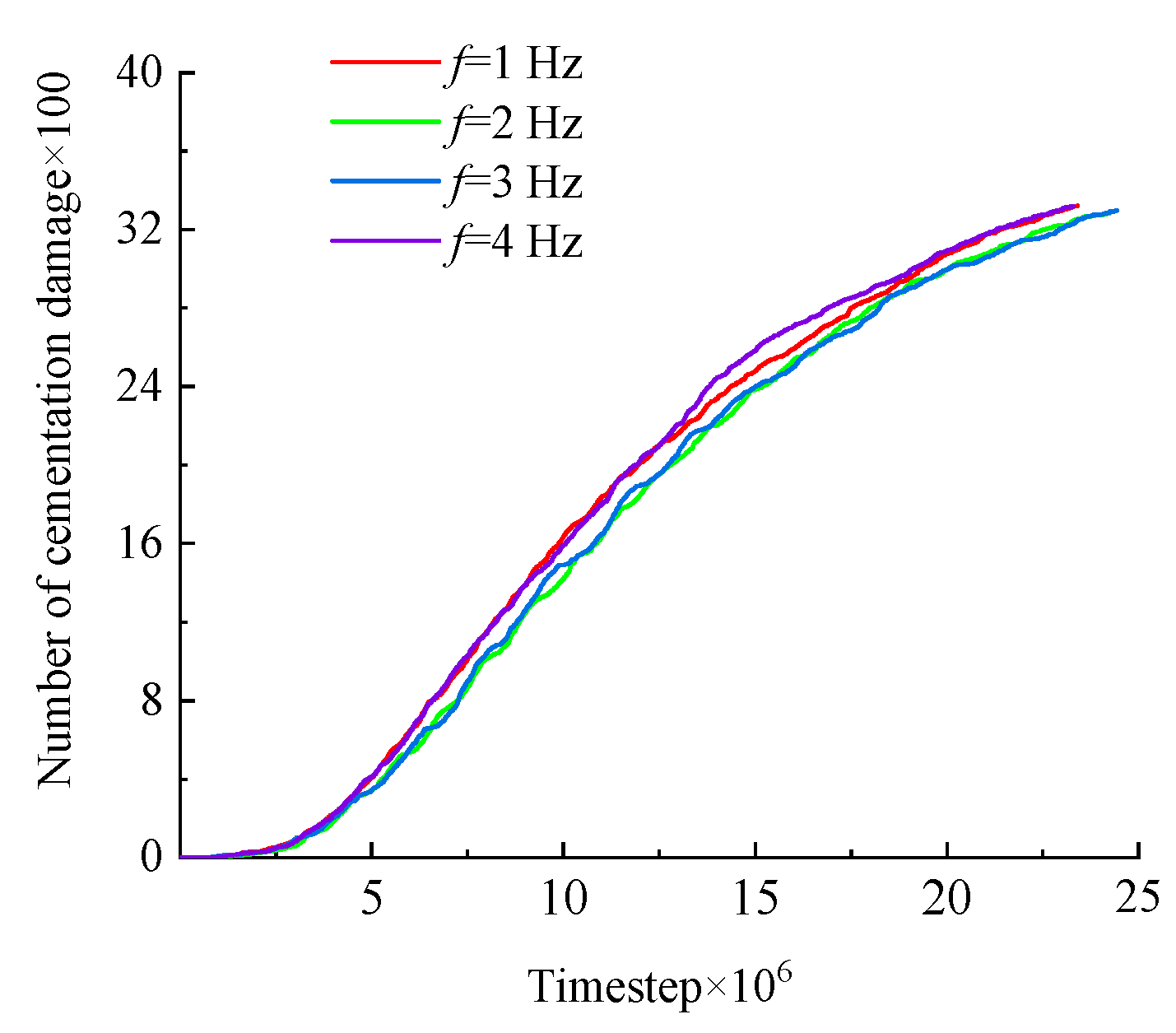
3.4.2. Effect of Loading Frequency

The simulation results under different frequency loading conditions at an amplitude of 0.12 m·s⁻¹ and an axial strain of 25% are shown in Figure 20. From the displacement cloud atlas in Figure 20a, it can be seen that when the loading frequency is less than γ (2 Hz < γ < 3 Hz), with the increase in loading frequency, the displacement of the middle particles within the model increases, and the distribution of the shear zone becomes less and less obvious. When the loading frequency is greater than γ, with the increase in loading frequency, the displacement of the middle particles within the model decreases, and the distribution of the shear zone becomes more and more obvious. By calculation, it can be obtained that the average stresses of the specimen are 1.334, 1.319, 1.323, and 1.344 MPa when f is 1, 2, 3, and 4 Hz, respectively. The lateral pressure and constraint provided by the wall on the particles are all the same under the same circumferential pressure, so with the axial stress getting smaller, the distribution of the shear zone is also becoming less and less obvious. On the contrary, the distribution of the shear zone is becoming more and more obvious. As shown in the Figure 20c microcrack expansion diagram, the less obvious the shear zone is, the less the number of cracks near the shear zone of the corresponding specimen. At the same time, in Figure 21, the curves of cementation damage–time step curves show the same trend for each loading frequency condition, and the number of cementation damage with time step for loading frequency conditions with similar average axial stresses has approximately the same law. The smaller the average axial stress is, the smaller the rate of cementation damage is. It can be seen that the damage to the cementation of specimens is closely related to the average axial stress to which they are subjected. As shown in the contact force chain cloud atlas in Figure 20b, when the loading frequency is less than β (2 Hz < β < 3 Hz), the color of the contact force chain between the particles in the shear zone becomes lighter, and the contact force decreases significantly with the increase in the loading frequency; when the loading frequency is greater than β, the contact force chain between the particles near the shear zone becomes more obvious, and the contact force increases significantly with the increase in the loading frequency. In the displacement cloud atlas, the greater the displacement of the particles, the more obvious the contact force chain, i.e., the greater the frictional resistance caused by particle dislocation, and on the contrary, the contact force chain is obviously reduced.

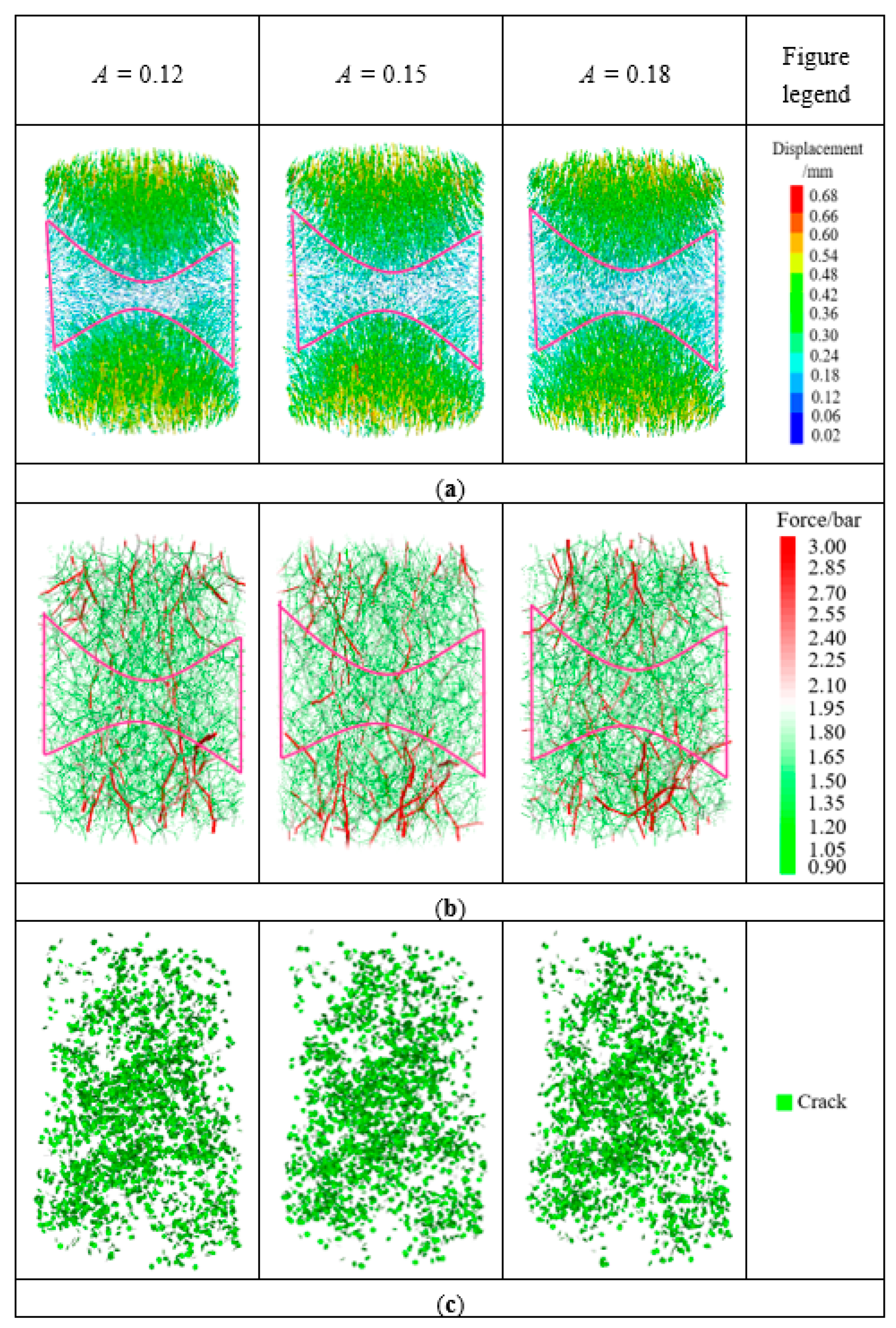
3.4.3. Effect of Loading Amplitude

The simulation results for different amplitude loading conditions at a frequency of 1 Hz and an axial strain of 25% are shown in Figure 22. The average stresses in the specimens were calculated to be 1.334, 1.387, and 1.394 MPa for loading amplitudes of 0.12, 0.15, and 0.18 m·s⁻¹, respectively. Combined with the displacement cloud in Figure 22a and the microcrack extension in Figure 22c, it can be seen that the average axial stress on the specimen increases with the increase in the loading amplitude. At this time, the displacement of the middle particles within the model decreases, the number of cracks increases, and the distribution of shear zones becomes more and more obvious. The reason is the same as the mechanism described in the previous section, so the larger the loading amplitude, the greater the axial stress, and the more obvious the distribution of the shear zone. As seen from the cementation damage–time step curve in Figure 23, with the increase in loading amplitude, both the number of cementation damage of the specimen and the damage rate increase. From the contact force chain atlas in Figure 22b, it can be seen that the contact force chain near the shear zone increases significantly with the increase in the loading amplitude, and the contact force chain between the particles is more obvious and increases significantly. Corresponding to the displacement cloud atlas, the greater the displacement of the particles, the more obvious the contact force chain, which means the greater the frictional resistance caused by the misalignment of the particles.

4. Conclusions

In this paper, numerical simulations of triaxial compression of hydrate sediment specimens under cyclic loading with different frequencies (1.2 × 10⁻¹, 1.5 × 10⁻¹, and 1.8 × 10⁻¹ m·s⁻¹) and amplitudes (1, 2, 3, and 4 Hz) were carried out to study the macroscopic mechanical properties of hydrate sediments under dynamic loading, revealing the effects of loading frequency and loading amplitude. The following main conclusions were obtained.

(1) The effect of loading frequency on the stiffness of hydrate sediment is small, but the effect on the peak strength is large and not monotonic. There is a critical value. When it is less than this value, the peak strength increases with the increase in loading rate, and when it is greater than this value, the peak strength decreases to a certain extent.

(2) The effect of loading amplitude on the peak strength and stiffness of hydrate sediments is monotonic. As the loading amplitude increases, the strength of the hydrate sediment specimens increases significantly, while the stiffness decreases.

(3) The loading frequency and amplitude have a large effect on the maximum shear dilatancy of sediment specimens, mainly due to the difference in the bearing capacity of the specimens because of the phase change point and particle rearrangement.

(4) The variation law of shear dilatancy angle with loading frequency for the sediment specimens is similar to that of shear dilatancy with loading frequency, which tends to increase linearly with the increase in loading amplitude.

(5) The effect of loading frequency and amplitude on the contact force chain, displacement, crack extension, and number of cementation damage inside the sediment is mainly related to the average axial stress to which the specimen is subjected. The higher the axial stress, the higher the rate of cementation damage, the more obvious the distribution of the shear zone of the specimen, and the more the number of cracks and cementation damage.

References

1. Guo, X.S.; Nian, T.K.; Zhao, W.; Gu, Z.D.; Liu, C.P.; Liu, X.L.; Jia, Y.G. Centrifuge experiment on the penetration test for evaluating undrained strength of deep-sea surface soils. Int. J. Min. Sci. Technol. 2022, 32, 363–373. [Google Scholar] [CrossRef]
2. Li, S.; Xu, X.; Zheng, R. Experimental investigation on dissociation driving force of methane hydrate in porous media. Fuel 2015, 160, 117–122. [Google Scholar] [CrossRef]
3. Guo, X.S.; Stoesser, T.; Nian, T.K.; Jia, Y.G.; Liu, X.L. Effect of pipeline surface roughness on peak impact forces caused by submarine mudflow. Ocean. Eng. 2021, 243, 110184. [Google Scholar] [CrossRef]
4. Masui, A.; Haneda, H.; Ogata, Y. Effects of methane hydrate formation on shear strength of synthetic methane hydrate sediments. Int. Soc. Offshore Polar Eng. 2005, 364–369. Available online: https://onepetro.org/ISOPEIOPEC/proceedings-abstract/ISOPE05/All-ISOPE05/ISOPE-I-05-056/9186 (accessed on 25 July 2022).
5. Hyodo, M.; Yoneda, J.; Yoshimoto, N. Mechanical and dissociation properties of methane hydrate-bearing sand in deep seabed. Soils Found. 2013, 53, 299–314. [Google Scholar] [CrossRef] [Green Version]
6. Song, Y.; Luo, T.; Madhusudhan, B.N. Strength behaviors of CH4 hydrate-bearing silty sediments during thermal decomposition. J. Nat. Gas Sci. Eng. 2019, 72, 103031. [Google Scholar] [CrossRef]
7. Wu, Q.; Lu, J.S.; Li, D.L. Mechanical characterization of hydrate-bearing sediments during decompression mining. Rock Soil Mech. 2018, 39, 4508–4516. [Google Scholar]
8. Kajiyama, S.; Hyodo, M.; Nakata, Y. Shear behavior of methane hydrate bearing sand with various particle characteristics and fines. Soils Found. 2017, 57, 176–193. [Google Scholar] [CrossRef]
9. Li, Y.; Dong, L.; Wu, N. Influences of hydrate layered distribution patterns on triaxial shearing characteristics of hydrate-bearing sediments. Eng. Geol. 2021, 294, 106375. [Google Scholar] [CrossRef]
10. Hao, L.K.; Shi, C.; Shan, Z.G. Numerical simulation of dynamic properties of marine soft soil under cyclic loading. J. China Three Gorges Univ. (Nat. Sci.) 2021, 43, 7. [Google Scholar]
11. Guo, X.S.; Nian, T.K.; Wang, D.; Gu, Z.D. Evaluation of undrained shear strength of surficial marine clays using ball penetration-based CFD modelling. Acta Geotech. 2022, 17, 1627–1643. [Google Scholar] [CrossRef]
12. Shen, Z.; Jiang, M.; Thornton, C. DEM simulation of bonded granular material. Part I: Contact model and application to cemented sand. Comput. Geotech. 2016, 75, 192–209. [Google Scholar] [CrossRef]
13. Cundall, P.A.; Strack, O.D.L. discrete numerical model for granular assemblies. Comput. Geotech. 1979, 29, 47–65. [Google Scholar] [CrossRef]
14. Dai, S.; Santamarina, J.C.; Waite, W.F. Hydrate morphology: Physical properties of sands with patchy hydrate saturation. J. Geophys. Res. 2012, 117, B11205. [Google Scholar] [CrossRef] [Green Version]
15. Bai, Q.; Konietzky, H.; Dang, W. Microscopic modeling of frictional response of smooth joint under normal cyclic loading. Rock Mech. Rock Eng. 2022, 55, 169–186. [Google Scholar] [CrossRef]
16. Li, X.; Zou, Y.; Zhou, Z. Numerical simulation of the rock shpb test with a special shape striker based on the discrete element method. Rock Mech. Rock Eng. 2014, 47, 1693–1709. [Google Scholar] [CrossRef]
17. Brugada, J.; Cheng, Y.P.; Soga, K. Discrete element modelling of geomechanical behavior of methane hydrate soils with pore-filling hydrate distribution. Granul. Matter 2010, 12, 517–525. [Google Scholar] [CrossRef]
18. Jiang, M.J.; Sun, Y.G.; Yang, Q.J. A simple distinct element modeling of the mechanical behavior of methane hydrate-bearing sediments in deep seabed. Granul. Matter 2013, 15, 209–220. [Google Scholar] [CrossRef]
19. Jiang, M.J.; Yu, H.S.; Harris, D. Bond rolling resistance and its effect on yielding of bonded granulates by DEM analyses. Int. J. Numer. Anal. Methods Geomech. 2006, 30, 723–761. [Google Scholar] [CrossRef]
20. Jiang, M.J.; Peng, D.; Ooi, J.Y. DEM investigation of mechanical behavior and strain localization of methane hydrate bearing sediments with different temperatures and water pressures. Eng. Geol. 2017, 223, 92–109. [Google Scholar] [CrossRef] [Green Version]
21. Jiang, M.J.; Liu, J.; Kwok, C.Y. Exploring the undrained cyclic behavior of methane-hydrate-bearing sediments using CFD–DEM. Comptes Rendus Mécanique 2018, 346, 815–832. [Google Scholar] [CrossRef]
22. Jiang, M.J.; Xiao, Y.; Zhu, F.Y. Study on micromechanical cementation model and parameters of deep-sea energy soil. Chin. J. Geotech. Eng. 2012, 34, 1574–1583. [Google Scholar]
23. Jung, J.W.; Santamarina, J.C.; Soga, K. Stress-strain response of hydrate-bearing sands: Numerical study using discrete element method simulations. J. Geophys. Res. Solid Earth 2012, 117, B04202. [Google Scholar] [CrossRef]
24. Yang, Q.J.; Zhao, C.F. Three-dimensional discrete element analysis of the mechanical properties of hydrate sediments. Rock Soil Mech. 2014, 35, 255–262. [Google Scholar]
25. He, J.; Blumenfeld, R.; Zhu, H. Mechanical behaviors of sandy sediments bearing pore-filling methane hydrate under different intermediate principal stress. Int. J. Geomech. 2021, 21, 04021043. [Google Scholar] [CrossRef]
26. Xie, Y.; Feng, J.; Hu, W. Deep-sea sediment and water simulator for investigation of methane seeping and hydrate formation. J. Mar. Sci. Eng. 2022, 10, 514. [Google Scholar] [CrossRef]
27. Cheng, Y.T. Triaxial compression mechanical behavior of the hydrate sediments based on particles arranged model. Model. Simul. 2018, 07, 199–208. [Google Scholar] [CrossRef]
28. Deng, B.Q. Discrete Element Triaxial Numerical Simulation Study of Irregular Gravelly Soil with Irregular Particles; Tianjin University Hydraulic Engineering: Tianjin, China, 2019. [Google Scholar]
29. Li, T.; Li, L.; Liu, J. Influence of hydrate participation on the mechanical behavior of fine-grained sediments under one-dimensional compression: A DEM study. Granul. Matter 2022, 24, 1–7. [Google Scholar] [CrossRef]
30. Wei, R.; Jia, C.; Liu, L. Analysis of the characteristics of pore pressure coefficient for two different hydrate-bearing sediments under triaxial shear. J. Mar. Sci. Eng. 2022, 10, 509. [Google Scholar] [CrossRef]
31. Liu, L.; Zhang, X.; Ji, Y. Acoustic wave propagation in a borehole with a gas hydrate-bearing sediment. J. Mar. Sci. Eng. 2022, 10, 235. [Google Scholar] [CrossRef]
32. Waite, W.F. Physical properties of hydrate-bearing sediments. Rev. Geophys. 2009, 47, 1–38. [Google Scholar] [CrossRef]
33. Potyondy, D.; Cundall, P. A bonded-particle model for rock. Int. J. Rock Mech. Min. Sci. 2004, 41, 1329. [Google Scholar] [CrossRef]
34. He, J.; Jiang, M.J. New method of discrete element formation and macromechanical properties of pore-filled deep-sea energy soils. J. Tongji Univ. (Nat. Sci.) 2016, 44, 709–717. [Google Scholar]
35. Ke, W. Study on Fatigue Damage Characteristics of Sandstone and Dynamic Influencing Factors of Slope Stability under Cyclic Dynamic Loading; Chongqing University Civil Engineering: Chongqing, China, 2018. [Google Scholar]
36. Guo, Z.W. Analysis of seismic wave modulus of asphalt pavement under accelerated loading. J. Highw. Transp. Res. Dev. 2014, 31, 6. [Google Scholar]
37. Lu, Z.H.; Qi, C.Z.; Jiang, K. Experimental study of shear swelling characteristics of sandy soils. Res. Explor. Lab. 2020, 39, 19–24. [Google Scholar]
38. Summary of Commonly Used Seismic Wave Data (72448 Seismic Wave-Hach.txt). Available online: https://download.csdn.net/download/weixin_44423448/14021977 (accessed on 15 April 2022).
39. Roscoe, K.H. The influence of strain in soil mechanics. Geotechnique 1970, 20, 129–170. [Google Scholar] [CrossRef]
40. He, J.; Jiang, M.J. Discrete element analysis of true triaxial test of macro and micro mechanical properties of pore-filled energy soils. Rock Soil Mech. 2016, 37, 3026–3034. [Google Scholar]
41. Wang, E.H. PFC3D Particle Flow Simulation of Mechanical Properties of Saturated Densified Muddy Sand; Nanchang University: Nanchang, China, 2019. [Google Scholar]
42. Zhang, Z.H. Meso-Scale Numerical Simulation of Triaxial Test of Coarse-Grained Soil Based on PFC3D; Sanxia University: Yichang, China, 2015. [Google Scholar]
43. Zhao, J.; Liu, C.; Li, C. Pore-scale investigation of the electrical property and saturation exponent of archive’s law in hydrate-bearing sediments. J. Mar. Sci. Eng. 2022, 10, 111. [Google Scholar] [CrossRef]
Figure 1. Gradation curves of discrete element samples and Toyoura sand (Adapted with permission from Ref. [26]. 2022, Xie, Y.; Feng, J.; Hu, W).
Jmse 10 01042 g001
Figure 2. Saturation and formation of hydrate bond of discrete element specimens of hydrate sediments.
Jmse 10 01042 g002
Figure 3. Realization method of dynamic load loading.
Jmse 10 01042 g003
Figure 4. This type of hydrate sediment bond (Adapted with permission from Ref. [32]. 2009, the American Geophysical Union); (a) Pore-filling; (b) Soil skeleton; (c) Bond.
Jmse 10 01042 g004
Figure 5. Schematic diagram of hydrate sediment contact model: (a) cemented cluster hydrate sediments; (b) schematic diagram of 3D cementation model.
Jmse 10 01042 g005
Figure 6. Schematic diagram of 3D parallel bonding model: (a) forces and moments transmitted by the bond (Adapted with permission from Ref. [32]. 2009, the American Geophysical Union); (b) failure criterion of classical parallel bonding model (Adapted with permission from Ref. [30]. 2022, Wei, R.; Jia, C.; Liu, L).
Jmse 10 01042 g006
Figure 7. Comparison of discrete element simulation results [17].
Jmse 10 01042 g007
Figure 8. (ag) the loading speed of each group of simulations.
Jmse 10 01042 g008
Figure 9. Stress–strain curve of hydrate sediments under dynamic loading (f = 2 Hz, A = 0.12 m·s−1).
Jmse 10 01042 g009
Figure 10. Stress–strain curves of sediment under different dynamic loads: (a) different loading frequencies; (b) different loading amplitudes.
Jmse 10 01042 g010
Figure 11. Relationship between sediment strain interval L and loading conditions (Stage I, Stage II): (a) different loading frequencies; (b) different loading amplitudes.
Jmse 10 01042 g011
Figure 12. Strain–time curves of sediment under different dynamic loads: (a) different loading frequencies; (b) different loading amplitudes.
Jmse 10 01042 g012
Figure 13. The relationship between the peak strength of sediment, E50, and the loading amplitude.
Jmse 10 01042 g013
Figure 14. The relationship between the peak strength of sediment, E50, and the loading amplitude.
Jmse 10 01042 g014
Figure 15. Volumetric strain-axial strain curves of sediment under different dynamic loads: (a) different loading frequencies; (b) different loading amplitudes.
Jmse 10 01042 g015
Figure 16. Relationship between maximum shear dilatation of sediment, loading frequency, and loading amplitude.
Jmse 10 01042 g016
Figure 17. Relationship between sediment dilatancy angle, loading frequency, and loading amplitude.
Jmse 10 01042 g017
Figure 18. Typical failure law of hydrate sediments under the dynamic load of f = 1.0 Hz and A = 0.12 m·s−1: (a) cloud diagram of sample particle displacement, (b) contact force chain diagram, and (c) microcrack expansion diagram.
Jmse 10 01042 g018
Figure 19. The stress–cementation failure–strain curve of hydrate sediments under dynamic load of f = 1.0 Hz and A = 0.12 m·s−1.
Jmse 10 01042 g019
Figure 20. Typical failure law of hydrate sediments with an axial strain of 25% under dynamic loads of different frequencies: (a) cloud atlas of sample particle displacement, (b) contact force chain atlas, and (c) microcrack expansion diagram.
Jmse 10 01042 g020
Figure 21. Failure–time step relationship of hydrate sediments cementation under different frequencies of dynamic loads.
Jmse 10 01042 g021
Figure 22. Typical failure laws of hydrate sediments with an axial strain of 25% under dynamic loads of different amplitudes: (a) cloud atlas of sample particle displacement, (b) contact force chain atlas, and (c) microcrack expansion diagram.
Jmse 10 01042 g022
Figure 23. Failure–time step relationship of hydrate sediments cementation under different frequencies of dynamic loads.
Jmse 10 01042 g023