
Accurate Fish Detection under Marine Background Noise Based on the Retinex Enhancement Algorithm and CNN


Abstract
:1. Introduction
2. Materials and Methods
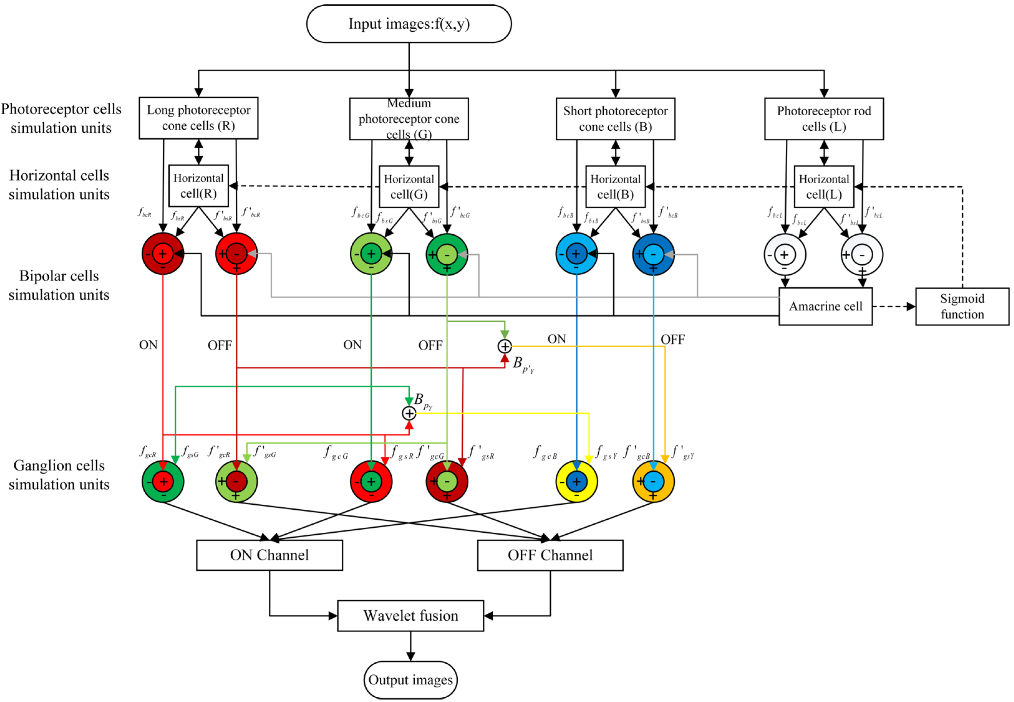
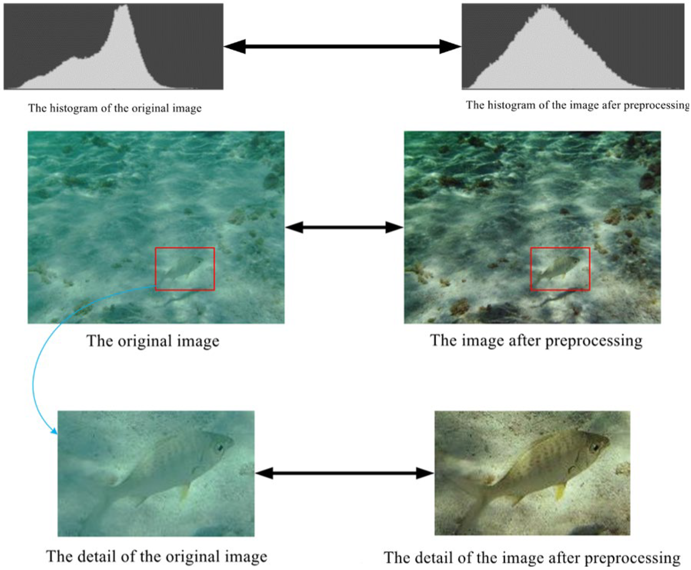
2.1. The Multi-Scale Retinex Enhancement Algorithm
2.2. The Multi-Scale Feature-Based Fish Detection Model
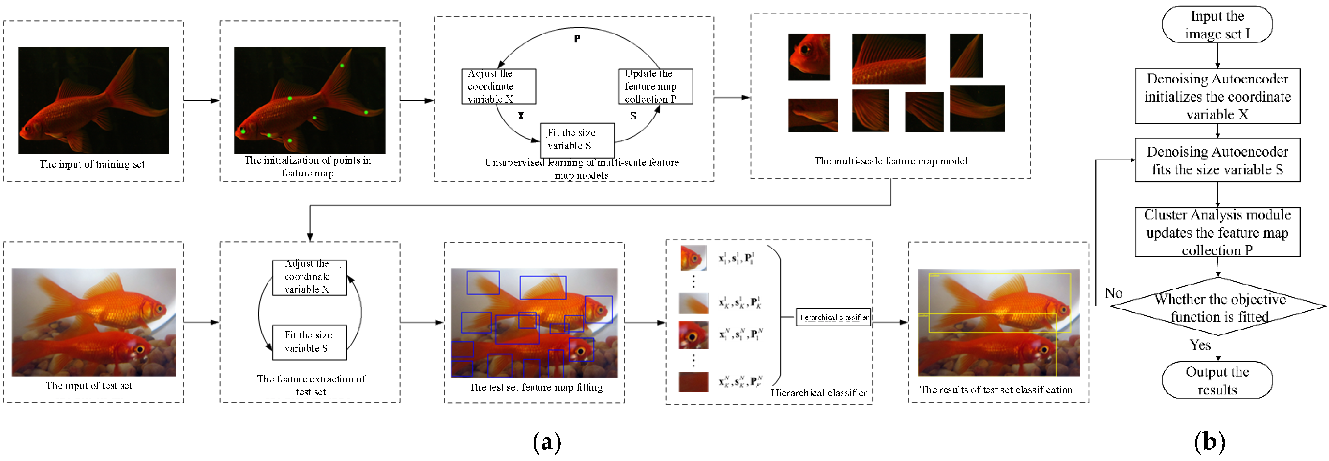
2.2.1. Feature Extraction Module
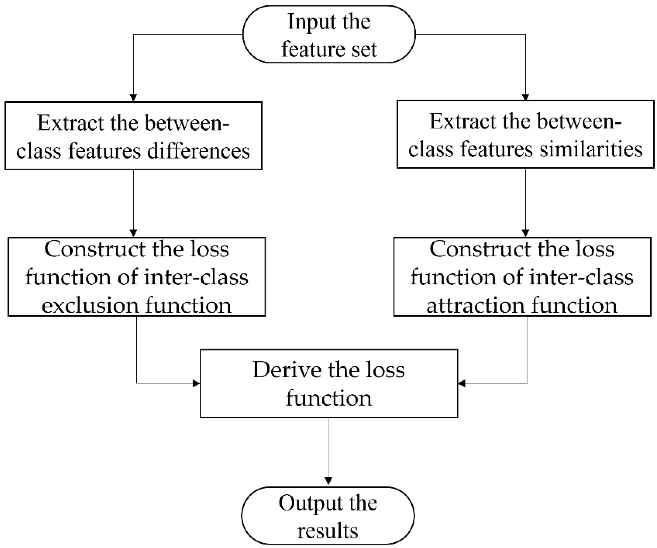
2.2.2. Region Proposal and Classification Module
3. Results
3.1. Experiment Setup
3.2. Result and Discussion
4. Conclusions
Author Contributions
Funding
Institutional Review Board Statement
Informed Consent Statement
Data Availability Statement
Conflicts of Interest
References
- Li, P. Research progress in high-value utilization of marine biological resources. Oceanol. Limnol. Sin. 2020, 51, 750–758. [Google Scholar] [CrossRef]
- Cong, Y.; Gu, C.; Zhang, T.; Gao, Y. Underwater robot sensing technology: A survey. Fundam. Res. 2021, 1, 337–345. [Google Scholar] [CrossRef]
- Girshick, R.; Donahue, J.; Darrell, T.; Malik, J. Rich Feature Hierarchies for Accurate Object Detection and Semantic Segmentation. In Proceedings of the IEEE Conference on Computer Vision and Pattern Recognition, Columbus, OH, USA, 23–28 June 2014; pp. 580–587. [Google Scholar] [CrossRef] [Green Version]
- Uijlings, J.R.R.; Van de Sande, K.E.A.; Gevers, T.; Smeulders, A.W.M. Selective Search for Object Recognition. Int. J. Comput. Vis. 2013, 104, 154–171. [Google Scholar] [CrossRef] [Green Version]
- He, K.; Zhang, X.; Ren, S.; Sun, J. Spatial Pyramid Pooling in Deep Convolutional Networks for Visual Recognition. IEEE Trans. Pattern Anal. Mach. Intell. 2015, 37, 1904–1916. [Google Scholar] [CrossRef] [PubMed] [Green Version]
- Girshick, R. Fast R-CNN. In Proceedings of the 2015 IEEE International Conference on Computer Vision (ICCV), Santiago, Chile, 7–13 December 2015; pp. 1440–1448. [Google Scholar] [CrossRef]
- Ren, S.; He, K.; Girshick, R.; Sun, J. Faster R-CNN: Towards Real-Time Object Detection with Region Proposal Networks. IEEE Trans. Pattern Anal. Mach. Intell. 2017, 39, 1137–1149. [Google Scholar] [CrossRef] [PubMed] [Green Version]
- Redmon, J.; Divvala, S.; Girshick, R.; Farhadi, A. You Only Look Once: Unified, Real-Time Object Detection. In Proceedings of the 2016 IEEE Conference on Computer Vision and Pattern Recognition (CVPR), Las Vegas, NV, USA, 27–30 June 2016; pp. 779–788. [Google Scholar] [CrossRef] [Green Version]
- Lin, C.-H.; Lin, Y.-S.; Liu, W.-C. An efficient license plate recognition system using convolution neural networks. In Proceedings of the 2018 IEEE International Conference on Applied System Invention (ICASI), Chiba, Japan, 13–17 April 2018; pp. 224–227. [Google Scholar] [CrossRef]
- Zhang, M.; Qiao, B.; Xin, M.; Zhang, B. Phase spectrum based automatic ship detection in synthetic aperture radar images. J. Ocean Eng. Sci. 2020, 6, 185–195. [Google Scholar] [CrossRef]
- Al-Aboosi, Y.Y.; Sha'Ameri, A.Z. Improved signal de-noising in underwater acoustic noise using S-transform: A performance evaluation and comparison with the wavelet transform. J. Ocean Eng. Sci. 2017, 2, 172–185. [Google Scholar] [CrossRef]
- Wang, H.; Zhang, S.; Zhao, S.; Wang, Q.; Li, D.; Zhao, R. Real-time detection and tracking of fish abnormal behavior based on improved YOLOV5 and SiamRPN++. Comput. Electron. Agric. 2021, 192, 106512. [Google Scholar] [CrossRef]
- Li, X.; Shang, M.; Qin, H.; Chen, L. Fast accurate fish detection and recognition of underwater images with Fast R-CNN. In Proceedings of the OCEANS 2015—MTS/IEEE Washington, Washington, DC, USA, 19–22 October 2015; pp. 1–5. [Google Scholar] [CrossRef]
- Cai, K.; Miao, X.; Wang, W.; Pang, H.; Liu, Y.; Song, J. A modified YOLOv3 model for fish detection based on MobileNetv1 as backbone. Aquac. Eng. 2020, 91, 102117. [Google Scholar] [CrossRef]
- Kottursamy, K. Multi-scale CNN Approach for Accurate Detection of Underwater Static Fish Image. J. Artif. Intell. Capsul. Netw. 2021, 3, 230–242. [Google Scholar] [CrossRef]
- Sung, M.; Yu, S.-C.; Girdhar, Y. Vision based real-time fish detection using convolutional neural network. In Proceedings of the OCEANS 2017-Aberdeen, Aberdeen, UK, 19–22 June 2017. [Google Scholar] [CrossRef]
- Levy, D.; Belfer, Y.; Osherov, E.; Bigal, E.; Scheinin, A.P.; Nativ, H.; Tchernov, D.; Treibitz, T. Automated Analysis of Marine Video with Limited Data. In Proceedings of the 2018 IEEE/CVF Conference on Computer Vision and Pattern Recognition Workshops (CVPRW), Salt Lake City, UT, USA, 18–22 June 2018; pp. 1466–14668. [Google Scholar] [CrossRef]
- Knausgård, K.M.; Wiklund, A.; Sørdalen, T.K.; Halvorsen, K.T.; Kleiven, A.R.; Jiao, L.; Goodwin, M. Temperate fish detection and classification: A deep learning based approach. Appl. Intell. 2021, 52, 6988–7001. [Google Scholar] [CrossRef]
- Ben Tamou, A.; Benzinou, A.; Nasreddine, K. Multi-stream fish detection in unconstrained underwater videos by the fusion of two convolutional neural network detectors. Appl. Intell. 2021, 51, 5809–5821. [Google Scholar] [CrossRef]
- Zhang, S.; Yang, X.; Wang, Y.; Zhao, Z.; Liu, J.; Liu, Y.; Sun, C.; Zhou, C. Automatic Fish Population Counting by Machine Vision and a Hybrid Deep Neural Network Model. Animals 2020, 10, 364. [Google Scholar] [CrossRef] [PubMed] [Green Version]
- Zheng, H.; Sun, X.; Zheng, B.; Nian, R.; Wang, Y. Underwater image segmentation via dark channel prior and multiscale hierarchical decomposition. In Proceedings of the OCEANS 2015-Genova, Genova, Italy, 18–21 May 2015; pp. 1–4. [Google Scholar] [CrossRef]
- Marburg, A.; Bigham, K. Deep learning for benthic fauna identification. In Proceedings of the OCEANS 2016 MTS/IEEE Monterey, Monterey, CA, USA, 19–23 September 2016; pp. 1–5. [Google Scholar] [CrossRef]
- Priyankan, K.; Fernando, T.G.I. Mobile Application to Identify Fish Species Using YOLO and Convolutional Neural Networks. In Proceedings of International Conference on Sustainable Expert Systems; Springer: Berlin/Heidelberg, Germany, 2021; pp. 303–317. [Google Scholar] [CrossRef]
- Song, M.; Qu, H.; Zhang, G.; Tao, S.; Jin, G. A Variational Model for Sea Image Enhancement. Remote Sens. 2018, 10, 1313. [Google Scholar] [CrossRef] [Green Version]
- Chen, W.; Wang, L.; Zhang, Y.; Li, X.; Liu, J.; Wang, W. Anti-disturbance grabbing of underwater robot based on retinex image enhancement. In Proceedings of the 2019 Chinese Automation Congress (CAC), Hangzhou, China, 22–24 November 2019; pp. 2157–2162. [Google Scholar] [CrossRef]
- Douglas, R.H.; Hawryshyn, C.W. Behavioural studies of fish vision: An analysis of visual capabilities. In The Visual System of Fish; Douglas, R., Djamgoz, M., Eds.; Springer: Dordrecht, The Netherlands, 1990; pp. 373–418. [Google Scholar] [CrossRef]
- Brown, C. Fish intelligence, sentience and ethics. Anim. Cogn. 2014, 18, 1–17. [Google Scholar] [CrossRef] [PubMed] [Green Version]
- Mangel, S.C.; Dowling, J.E. The interplexiform–horizontal cell system of the fish retina: Effects of dopamine, light stimulation and time in the dark. Proc. R. Soc. Lond. Ser. B Biol. Sci. 1987, 231, 91–121. [Google Scholar] [CrossRef]
- Angelucci, A.; Bijanzadeh, M.; Nurminen, L.; Federer, F.; Merlin, S.; Bressloff, P.C. Circuits and Mechanisms for Surround Modulation in Visual Cortex. Annu. Rev. Neurosci. 2017, 40, 425–451. [Google Scholar] [CrossRef]
- Fisher, R.; Chen-Burger, Y.; Giordano, D.; Hardman, L.; Lin, F. Fish4Knowledge: Collecting and Analyzing Massive Coral Reef Fish Video Data; Springer: Heidelberg, Germany, 2016. [Google Scholar]


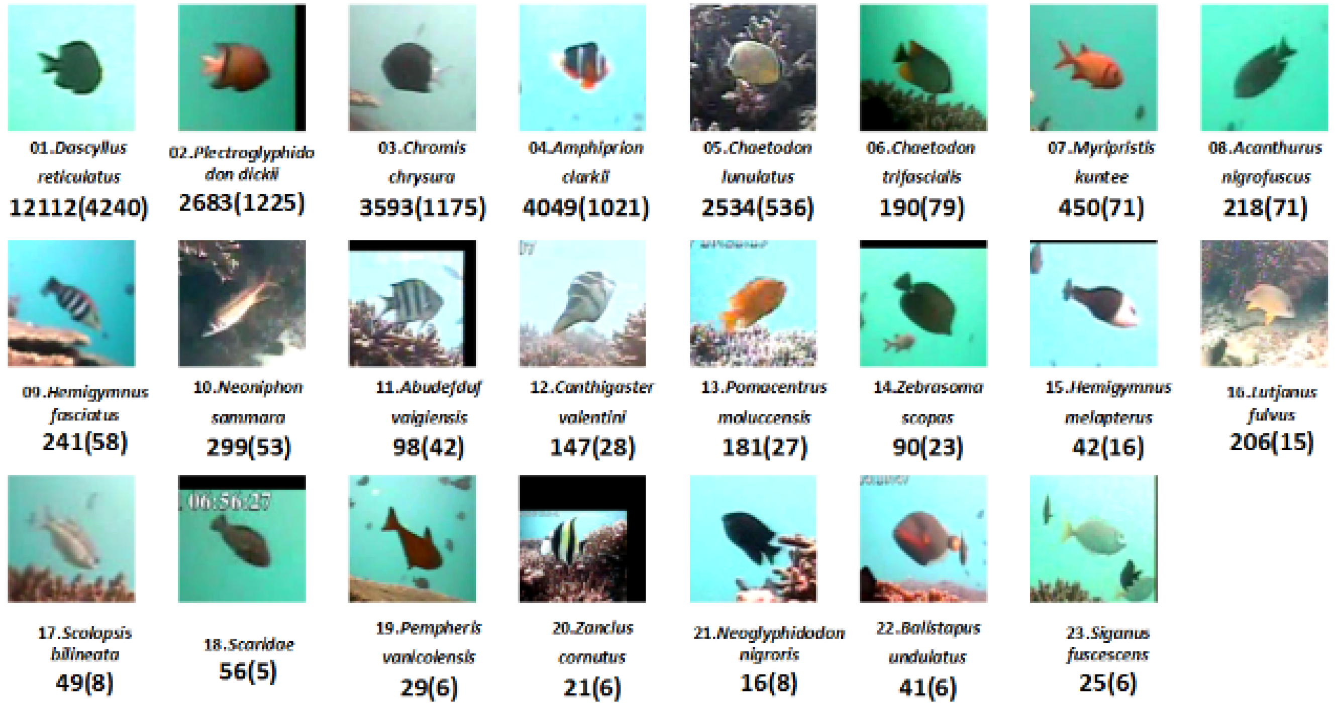
| Fish Species | Training Set | Validation Set | Test Set |
|---|---|---|---|
| dascyllus reticulatus | 4032 | 4042 | 4037 |
| plectroglyphido don dickii | 894 | 890 | 898 |
| chromis chrysura | 1192 | 1202 | 1197 |
| amphiprion clarkii | 1349 | 1355 | 1344 |
| chaetodon lunulatus | 844 | 839 | 849 |
| chaetodon trifascialis | 63 | 68 | 58 |
| myripristis kuntee | 145 | 155 | 150 |
| acanthurus nigrofuscus | 78 | 68 | 73 |
| hemigymnus fasciatus | 85 | 75 | 80 |
| neoniphon sammara | 94 | 104 | 99 |
| canthigaster valentini | 44 | 54 | 49 |
| pomacentrus moluccensis | 55 | 65 | 60 |
| lutjanus fulvus | 63 | 73 | 68 |
| total number of sample | 8938 | 8990 | 8962 |
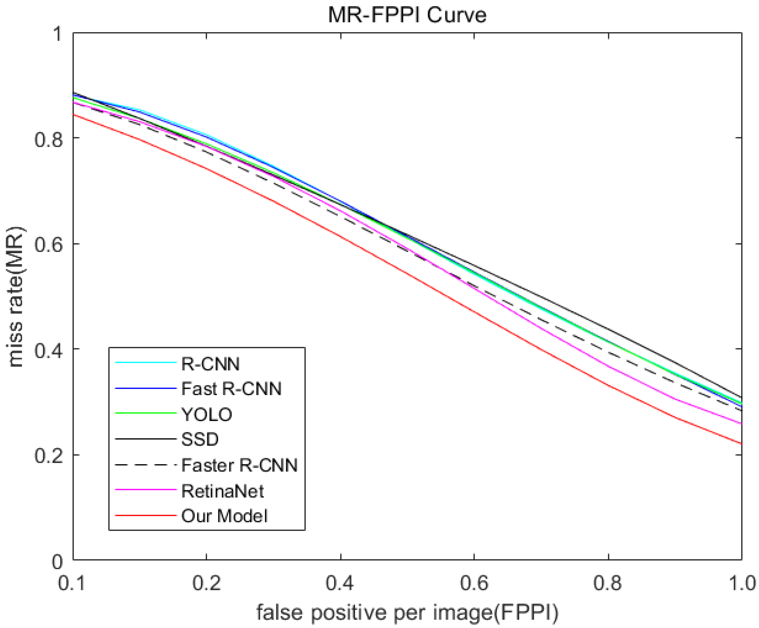
| Method | mMR | Improvement |
|---|---|---|
| R-CNN | 63.42 | / |
| Fast R-CNN | 63.30 | 0.12 |
| YOLO | 63.20 | 0.22 |
| SSD | 62.76 | 0.66 |
| Faster R-CNN | 60.82 | 2.60 |
| RetinaNet | 59.44 | 3.96 |
| Our Model | 54.11 | 9.31 |
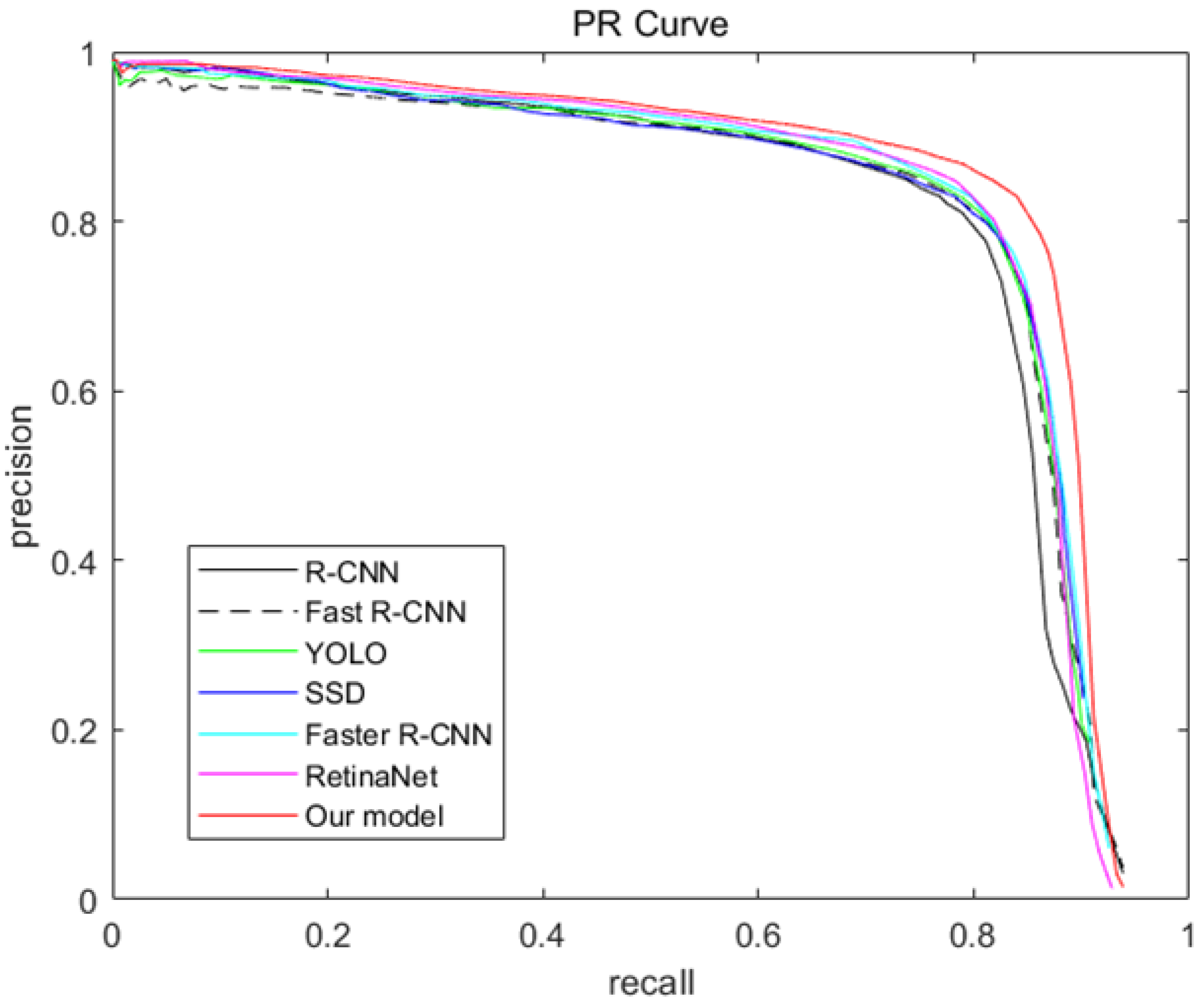
| Method | mAP | Improvement |
|---|---|---|
| R-CNN | 70.29 | / |
| Fast R-CNN | 71.56 | 1.27 |
| YOLO | 71.81 | 1.52 |
| SSD | 72.24 | 1.95 |
| Faster R-CNN | 72.97 | 2.68 |
| RetinaNet | 73.03 | 2.74 |
| Our Model | 78.31 | 8.02 |
Publisher’s Note: MDPI stays neutral with regard to jurisdictional claims in published maps and institutional affiliations. |
© 2022 by the authors. Licensee MDPI, Basel, Switzerland. This article is an open access article distributed under the terms and conditions of the Creative Commons Attribution (CC BY) license (https://creativecommons.org/licenses/by/4.0/).
Share and Cite
Chen, Y.; Ling, Y.; Zhang, L. Accurate Fish Detection under Marine Background Noise Based on the Retinex Enhancement Algorithm and CNN. J. Mar. Sci. Eng. 2022, 10, 878. https://doi.org/10.3390/jmse10070878
Chen Y, Ling Y, Zhang L. Accurate Fish Detection under Marine Background Noise Based on the Retinex Enhancement Algorithm and CNN. Journal of Marine Science and Engineering. 2022; 10(7):878. https://doi.org/10.3390/jmse10070878
Chicago/Turabian StyleChen, Yanhu, Yucheng Ling, and Luning Zhang. 2022. "Accurate Fish Detection under Marine Background Noise Based on the Retinex Enhancement Algorithm and CNN" Journal of Marine Science and Engineering 10, no. 7: 878. https://doi.org/10.3390/jmse10070878
APA StyleChen, Y., Ling, Y., & Zhang, L. (2022). Accurate Fish Detection under Marine Background Noise Based on the Retinex Enhancement Algorithm and CNN. Journal of Marine Science and Engineering, 10(7), 878. https://doi.org/10.3390/jmse10070878