Article

Investigation of Vortex Structure Modulation by Spume Droplets in the Marine Atmospheric Boundary Layer by Numerical Simulation

1
Institute of Applied Physics of the Russian Academy of Sciences, Nizhny Novgorod 603950, Russia
2
Department of Engineering Science and Ocean Engineering, National Taiwan University, Taipei 10617, Taiwan
*
Author to whom correspondence should be addressed.
J. Mar. Sci. Eng. 2022, 10(7), 856; https://doi.org/10.3390/jmse10070856
Submission received: 26 May 2022 / Revised: 16 June 2022 / Accepted: 21 June 2022 / Published: 23 June 2022
(This article belongs to the Special Issue Numerical Modelling of Atmospheres and Oceans)

Abstract

:
Direct numerical simulation (DNS) of a droplet-laden, turbulent Couette airflow over a waved water surface is performed modeling the marine atmospheric boundary (MABL) layer carrying idealized spume droplets. Both the instantaneous and mean flow properties, the characteristics of the vortex structures and the momentum exchange between air turbulence and waved water surface and droplet-mediated momentum transfer are investigated. A Eulerian–Lagrangian approach is employed in DNS where full, 3D Navier–Stokes equations for the carrier air are solved in a Eulerian frame, and the trajectories of individual droplets are simultaneously tracked in a Lagrangian frame. The impact of the droplets on the carrier air flow is modeled via a point force approximation. The droplets size is considered in the range of spume droplet sizes observed in MABL. Various water surface roughness and droplet injection scenarios are considered, and both instantaneous and phase-averaged flow fields, the Reynolds stresses and the eigenvalues of the local air velocity gradient tensor are evaluated in DNS. Numerical results show a strong dependence of the droplet-mediated airflow modification on-the-droplet injection mechanism. Droplets injected with the surrounding air velocity effectively mitigate the vortex structures by reducing their swirling strength and suppress the momentum flux from air turbulence to water surface by weakening both ejections and sweeping events, and thus accelerating the mean flow as compared to the droplet-free flow. On the other hand, droplets injected with the velocities of the Lagrangian particles of the water surface enhance both the swirling strength of the vortex structures and air-flow turbulent stresses and decelerate the mean wind. The results also show that these effects of droplet-mediated flow modification become less pronounced as the water surface wave steepness increases.

1. Introduction

Large-scale prognostic models predicting bulk properties of the marine atmospheric boundary layer (MABL) are based on parameterizations of turbulent transfer fluxes of momentum, mass and heat and require detailed knowledge of small-scale exchange processes occurring in the vicinity of the air–sea interface [1]. A turbulent boundary layer developing near the water surface is characterized by the presence of coherent vortex structures, which contribute to the air–water momentum flux and influence the surface drag [2]. Direct measurements of droplet-mediated exchange fluxes in the vicinity of the air–water interface in field conditions and laboratory experiments are technically difficult due to the unsteadiness of the water surface in the presence of wave motions [3]. Investigation of this flow area in the field often becomes even more complicated by air-born sea-spray droplets, which interfere with air–sea interaction and exchange fluxes [4,5,6].
Direct numerical simulation represents an effective research tool and has been successfully employed in the studies of boundary layer flows in the vicinity of waved boundaries, both in droplet-free [7,8,9,10,11] and droplet-laden cases [12,13]. Although the bulk airflow Reynolds numbers in these numerical experiments are typically by orders of magnitude below the values observed in natural MABL, the results provide valuable knowledge of droplet-mediated exchange fluxes, which can be further used in large-scale prognostic models [14]. However, the impact of droplets on the carrier vortex structures has been investigated in detail only for flows over flat (solid) boundaries [15,16]. In these studies, a swirling strength of coherent vortices was explored by evaluating imaginary eigenvalues of the velocity gradient tensor, whereas a quadrant analysis of the velocity field was based on conditional averaging of turbulent velocity fluctuations. These studies show that, under considered conditions and injection scenarios, inertial particles reduce both swirling strength and the number of sweep and ejection events in the boundary layer as compared to the unladen flow case. These findings seem to corroborate an assumption that the impact of sea-spray droplets on MABL may be regarded as a possible reason for the drag reduction observed in hurricanes [6,17]. However, many aspects of the vortex structure modification, related both to the influence of water surface roughness and different possible scenarios of droplets injection, have still remained unexplored.
The objective of this study is to perform direct numerical simulation (DNS) of a turbulent, droplet-laden Couette airflow over a waved water surface. This flow can be regarded as an idealized model of the marine atmospheric boundary layer [7]. Both the instantaneous and mean flow properties and the net impact of the dispersed droplets on the vortex structures and the momentum exchange between air turbulence and water surface are investigated. A Eulerian–Lagrangian approach is adopted where full, 3D Navier–Stokes equations for the carrier air are solved in a Eulerian frame, and the trajectories of individual droplets are simultaneously tracked in a Lagrangian frame. The impact of the droplets on the carrier airflow is modeled via a point force approximation. The droplets diameter is considered in the range of spume droplets sizes observed in the laboratory experiment [18] (typically around 200 micron), which allows us to disregard effects related to droplets deformation. Both instantaneous and phase-averaged flow fields, the Reynolds stresses and the eigenvalues of the local air velocity gradient tensor for two surface wave slope are evaluated for two different droplet injection scenarios. The numerical method is based on an algorithm previously developed for modeling droplet-laden atmospheric boundary layers over progressive surface waves [12] and further adopted below for evaluating the impact of the dispersed spray on MABL vortex structures and air–sea momentum transfer.

2. Governing Equations

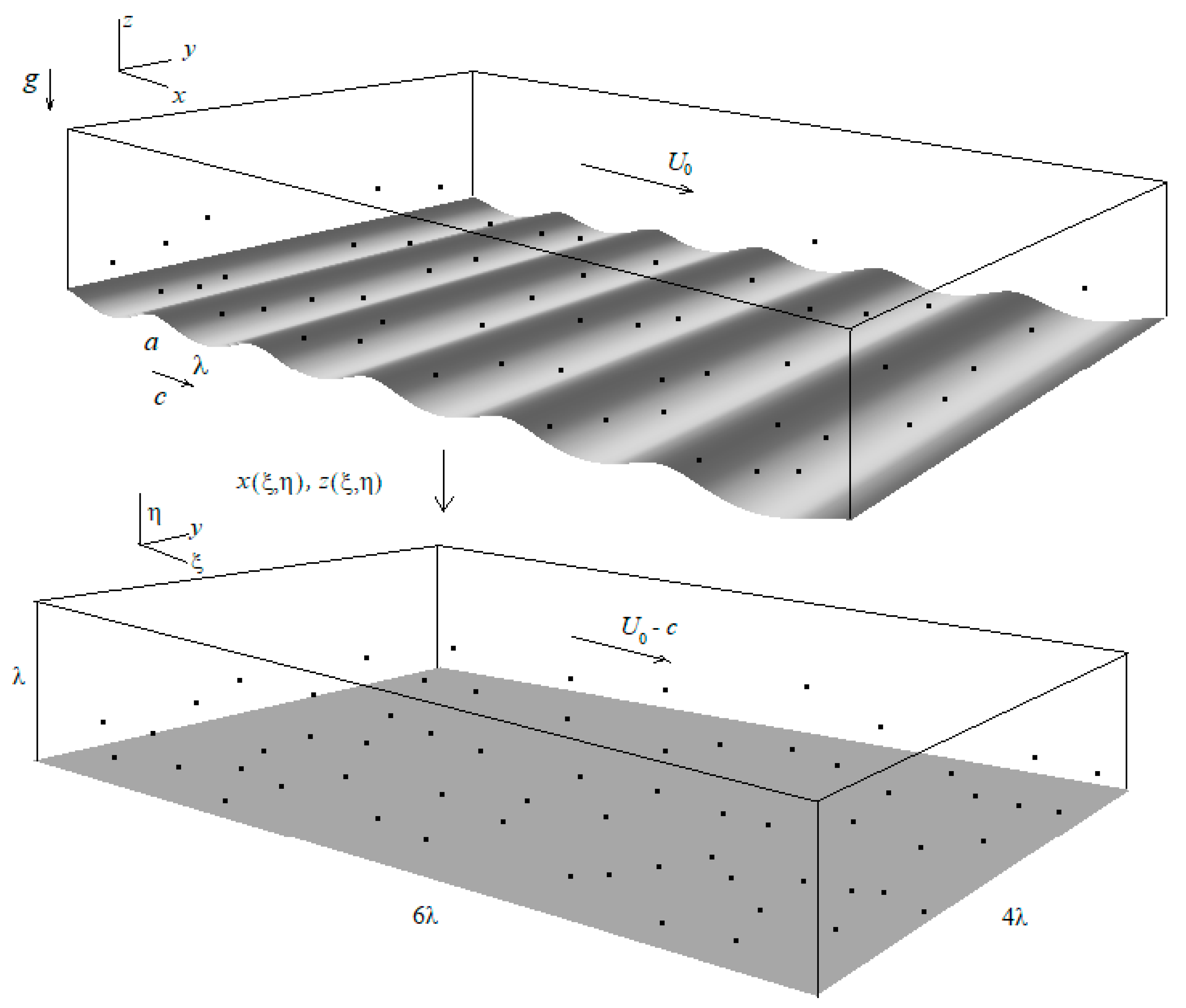
The schematic of the problem under consideration is similar to the settings in the previous DNS study [12] (Figure 1). A physical domain with sizes L x = 6 λ , L y = 4 λ , L z = λ , with periodic side boundaries, a solid, flat upper boundary and a waved bottom boundary, z s ( x , t ) , is considered where the Cartesian coordinates are employed, 0 x L x ; L y / 2 y L y / 2 ; z s z L z . The motion of the air is driven by the upper boundary moving with bulk velocity, U 0 , and also by the bottom boundary in the form of a prescribed, progressive, two-dimensional (2D) stationary wave of amplitude a, celerity c and length λ propagating in the positive x-direction. The wave celerity is considered sufficiently small (c/U0 = 0.05, c / u 1.5 where u 0.03 U 0 is the air friction velocity), which is characteristic of “slow” waves as compared to the wind, which is typical under strong wind-forcing conditions [7,8]. In order to avoid coping with a strong geometric nonlinearity caused by the wavy boundary during the integration of the governing equations (to be discussed below), a mapping is introduced transforming the physical domain into a computational domain with a flat bottom boundary, and relating the Cartesian coordinates (x, z) to curvilinear coordinates ( ξ , η ) as:
x = ξ a exp ( k η ) sin k ξ , z = η + a exp ( k η ) cos k ξ ,
where k = 2 π / λ is the wavenumber. Mapping (1) transforms the wavy boundary at z = z s ( x , t ) into a flat-plane boundary at η = 0 (Figure 1). The water surface elevation, z s ( x , t ) , is defined implicitly by Equation (1) and up to the second order in ka coincides with the Stokes wave solution [19]:
z s ( x , t ) a cos k ( x c t ) + a 2 k 2 cos 2 k ( x c t )
An additional mapping is also employed for the vertical coordinate in the form:
η / λ = 1 2 ( 1 + tanh η ˜ tanh 1.5 ) ,
where 1.5 η ˜ 1.5 , so that the grid nodes are clustered in the vicinity of the upper and bottom boundary, at η = 0 ( η ˜ = 1.5 ) and η = λ ( η ˜ = 1.5 ), and stretched towards the middle of the domain (at η = 0.5 λ , η ˜ = 0 ). The computations are preformed in a reference frame moving with the wave celerity c where the bottom boundary is stationary. Periodic and Dirichlet conditions (to be specified below) are considered at the side and upper and bottom boundary planes, respectively.
A Eulerian–Lagrangian approach is adopted where full, 3D Navier–Stokes equations of the water motion are solved in a Eulerian frame, and the droplets are tracked simultaneously by solving their respective equations of motion in a Lagrangian frame. The Navier–Stokes equations for the carrier air are written in the dimensionless form [1,12,20]:
U i t + ( U i U j ) x j = P x j + 1 Re 2 U i x j x j + n = 1 N d S i n
where x i ( x , y , z ) , U j = ( U x , U y , U z ) are the air velocity components, P is the pressure, and S i n is a momentum source term (cf. Equation (8) below) contributed by the n-th droplet, and n = 1, …, N d , the latter being the total, constant and number of tracked droplets. Variables in Equation (4) are normalized with velocity scale, U0, and length scale equal to the wave length, λ. The pressure is normalized with ρ U 0 2 where ρ is the air density (≈1.2 kg/m3). The airflow Reynolds number, Re, measures the ratio of the inertial vs. viscous effects and is defined as:
Re = U 0 λ ν
where ν is the air kinematic viscosity (≈1.5 × 10⁻⁵ m2/s). Equation (4) is supplemented by the incompressibility condition:
U j x j = 0 ,
which implicitly defines the pressure field, P (cf. Equation (18) below).
The droplets equations of motion are written as [21]:
d r i n d t = V i n ,
d V i n d t = f ( Re n ) τ ( U i n V i n ) + g δ i z .
In Equations (7) and (8), r i n , V i n ( i = x , y , z ) are the n-th droplet coordinate and velocity components, U i n is the air velocity at the droplet location, d / d t is the material derivative along the droplet trajectory; g is a dimensionless gravitational acceleration (to be defined below), and δ i j is the Kronecker tensor. The correction in the viscous drag force (accounted for by factor f) is caused by a finite Reynolds number of the droplet and defined as:
Re n = d | U n V n | ν ,
where [21]
f ( Re n ) = ( 1 + 0.15 Re n 0.687 ) .
Dimensionless time scale τ in the drag force on the right hand side of Equation (8) characterizes the ability of the droplet to follow variations of the surrounding air velocity and is defined as:
τ = d 2 18 ν ρ d ρ U 0 λ .
Notice that other forces on the droplet by the surrounding carrier air (pressure gradient, added mass, Basset and lift) are neglected as compared to the drag force in the considered case of large droplet-to-air density ratio, ρ d / ρ 10 3 , and a sufficiently small droplet diameter (d = 200 µm) [21,22]. Note also that the chosen droplet diameter in DNS is smaller as compared to the viscous (“wall”) length scale (to be discussed below), and the droplet can be treated as a point particle.
The momentum source term in the right hand side of Equation (4), S i n , is formulated adopting a “point force” approximation [12]:
S i n = π d 3 6 ρ d ρ 1 τ ( V i n U i ( r n ) ) ( 1 + 0.15 Re n 0.687 ) w ( r n , r ) Ω g ,
where w ( r n , r ) is a geometrical weight-factor inversely proportional to the distance between the n-th droplet located at rn = (xn, yn, zn) and the grid node at r = (x, y, z), and Ωg (r) is the volume of the considered grid cell. Thus, for each individual droplet, eight weight-factors are defined (for each of the surrounding grid nodes) and normalized, so that the sum of partial contributions distributed to these nodes exactly equals the respective total source contribution. Therefore, there is no numerically induced loss or gain of momentum in the droplet–air exchange process (cf., e.g., [12] and references therein for a more detailed discussion).

3. Numerical Method

Since the mapping, Equation (1), is conformal, the following relations between the derivatives hold:
x ξ = 1 J ξ x = z η = 1 J η z ; x η = 1 J ξ z = z ξ = 1 J η x ,
where the Jacobian of the transformation is:
J = ( ξ x ) 2 + ( ξ z ) 2 .
Due to the properties in Equations (13) and (14), the derivatives over the Cartesian coordinates, x and z, can be related to the derivatives over curvilinear coordinates, ξ , η , as
x = ξ x ξ + η x η = J ( x ξ ξ + x η η ) , z = ξ z ξ + η z η = J ( z ξ ξ + z η η ) .
The Laplacian operator is also rewritten as:
2 x j x j = J ( 2 ξ 2 + 2 η 2 ) + 2 y 2
Equations (4) and (6) for the air velocity are discretized on a staggered grid consisting of 360 × 240 × 180 nodes, in the ξ , y and η ˜ coordinate directions using a second order accuracy finite difference method. The integration of Equation (4) is advanced in time by the second order accuracy Adams–Bashforth method in two stages to calculate the air velocity at each new time step, Ui(tk+1). First, an intermediate velocity, U i , is computed using the velocity fields at the preceding time steps [23]:
U i = U i ( t k ) + ( 3 2 F i ( t k ) 1 2 F i ( t k 1 ) ) Δ t ,
where the flux, F i , is evaluated as
F i = ( U i U j ) x j + 1 Re 2 U i x j x j + n = 1 N b S i n .
Further, the new pressure, P ( t k + 1 ) , is computed by solving its respective Poisson equation in the form
2 P ( t k + 1 ) x j x j = 1 Δ t U j x j .
Equation (19) is solved by iterations by performing; at each iteration step (j) the FFT in the horizontal directions and Gaussian elimination in the vertical direction. The iteration procedure stops when the condition | P j + 1 P j | / P j < 0.1 % is satisfied. Usually, this condition is met after 3–5 iterations [12]. The new velocity at k + 1 time step satisfying the incompressibility condition (6) is then computed as:
U i ( t k + 1 ) = U i P ( t k ) x j Δ t .
At the bottom boundary, η = 0 , the Dirichlet condition for the air velocity is prescribed to be equal to the surface wave velocity [1] (minus the wave celerity):
U x ( ξ , y , 0 ) = c ( k a   cos k x ( ξ , 0 ) 1 ) , U y ( ξ , y , 0 ) = 0 , U x ( ξ , y , 0 ) = c k a   sin k x ( ξ , 0 ) .
Periodic conditions for all the fields are prescribed at the side boundaries, and the Dirichlet condition for the air velocity is prescribed at the upper boundary, η = 1 , moving with the dimensionless bulk velocity:
U x ( ξ , y , 1 ) = 1 c , U y ( ξ , y , 1 ) = 0 , U z ( ξ , y , 1 ) = 0 .
The droplet equation of motion is solved by employing the Adams–Bashforth method:
V i n ( t k + 1 ) = V i n ( t k ) + ( 3 2 F i n ( t k ) 1 2 F i n ( t k 1 ) ) Δ t ,
F i n = f ( Re n ) τ ( U i n V i n ) g δ i z .
In Equation (23), the surrounding air velocity at the location of each droplet is obtained via the Hermitian 4th-order accuracy interpolation procedure. The droplet coordinate equation is advanced in time by employing the Adams method as:
r i n ( t k + 1 ) = r i n ( t k ) + 0.5 ( V i n ( t k + 1 ) + V i n ( t k ) ) Δ t
If a droplet leaves the computational domain via the side boundary plane, it re-enters the domain at the respective opposite side boundary with the same z-coordinate and velocity due to periodicity in x and y directions. If the droplet either reaches the bottom boundary plane (the water surface, η = 0) or the upper horizontal moving plane (at η = 1 ) it is re-injected into the flow. Natural and laboratory observations show that spume drops are typically injected in the vicinity of wave crests [18,24,25]. In the present study, the injection model employed in [12] is used: the droplets are injected at heights 0.01 < η < 0.05 (or 5 < η ν / u < 25 
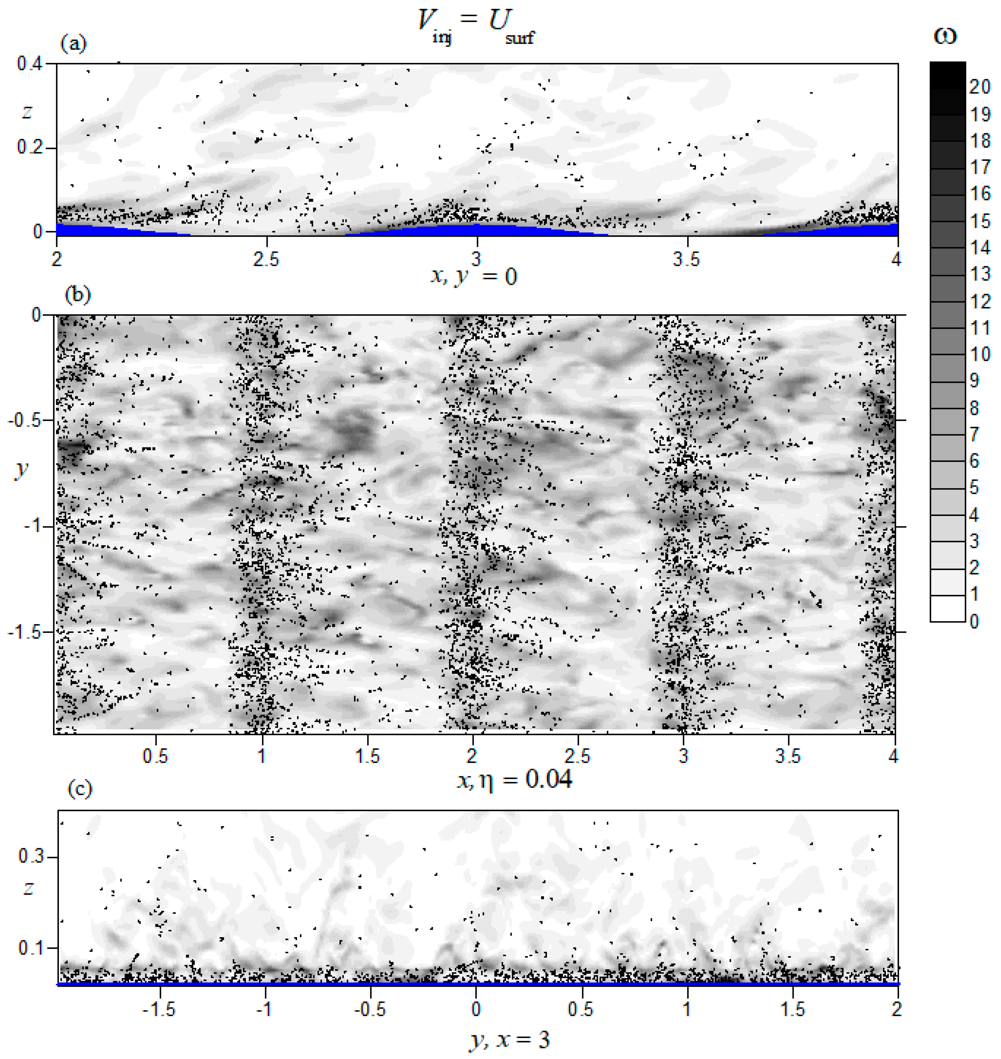
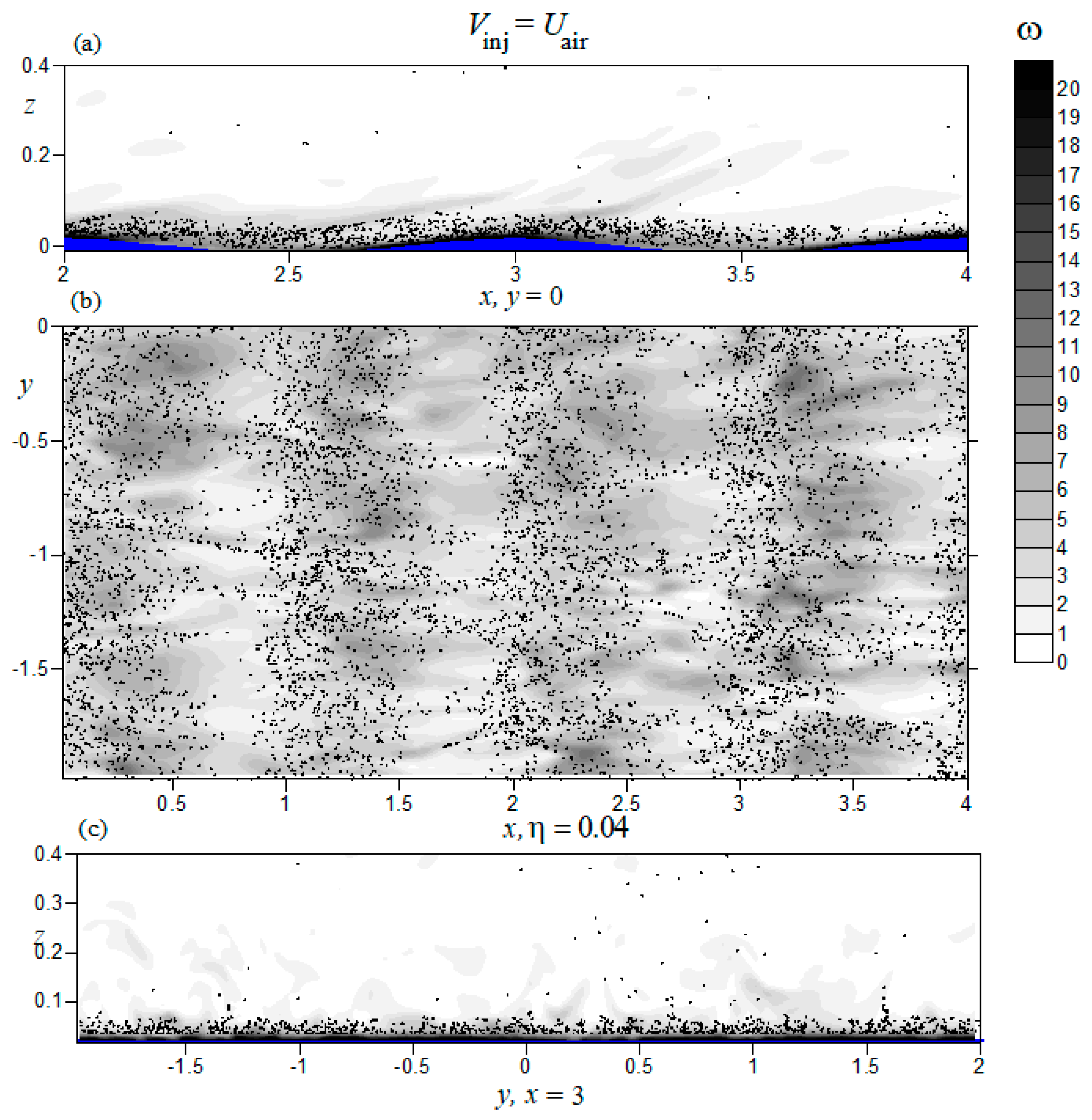
in the wall units) above the water surface and randomly distributed at upwind wave slopes in the vicinity of the wave crests. The statistics of spume droplets initial velocity distribution at present are not yet known. Therefore, two different types of injection scenario are considered. Under the first scenario, the droplet velocity at injection equals the surrounding air velocity (the case V i n j = U a i r ). Under the alternative scenario, the droplet velocity at injection equals the orbital velocity of the water surface particle in an irrotational two-dimensional deep-gravity wave at given x coordinate, Equation (21), ( V i n j = U s u r f ). These two cases of droplet injection are modeled separately.
The airflow bulk Reynolds number in DNS, Equation (5), is set equal to Re = 15,000. The corresponding friction Reynolds number equals Re = u λ / ν 500 , and is sufficiently large and allows a fully developed turbulent airflow. Experimental observations [25] indicate that for spume droplets with diameters around 200 μ m , the ratio of the terminal settling velocity, V s = τ g (where τ is given by Equation (11) vs. the product of the von Kármán constant and the friction velocity, κ u ), is of the order of unity. Thus, the dimensionless gravitational acceleration, g, is prescribed in DNS to satisfy this condition [12].
The air velocity field is initiated as a weakly perturbed, laminar Couette flow. During an initial transient, 0 < t < 100 , the source terms due to drops on the r. h. s. of Equation (4) is set to zero, and a fully developed turbulent, unladen flow regime sets in. At time t = 100 , droplets are introduced into the flow, with the total (constant) number Nd = 3 × 10⁶, and the initial uniform mass fraction is about 0.038. The droplet volume fraction remains far below 10−4 and allows neglecting hydrodynamic interactions between neighbouring droplets. The equations of motion of air and droplets, Equations (4)–(8), are solved simultaneously during the time interval 100 < t < 150 with the source term “turned off”. During this transient, the droplet dynamics adjusts to the airflow dynamics. At later times, 150 < t < 200 , the airflow and droplet equations of motion are solved with the source terms “turned on”. During this time interval, a statistically stationary, droplet-laden, two-way coupled flow regime is established.
Similarly, to the previous DNS studies of flows over waved surfaces [7,8,9,10,11,12,13], in the statistical post-processing analysis, phase averaging, equivalent to averaging over an ensemble of turbulent fluctuations, is performed. This averaging (denoted below by angular brackets) is firstly performed over y-coordinate and time t, and further window averaged over ξ—coordinate over six wave lengths as:
F ( ξ , η ) = 1 6 N t N y j = 1 N y k = 1 N t m = 0 5 F ( ξ + m λ , y j , λ η , t k )
where F is the averaged field, N y = 240 . Time averaging is preformed over N t = 500 realizations in the interval 200 < t k 300 . Further, the mean vertical profile of 〈F〉 is obtained by additional averaging along the ξ-coordinate as:
[ F ] ( η ) = 1 N x / 6 l = 1 N x / 6 F ( ξ l , η ) ,
where Nx = 360.
The averaging procedure outlined in Equations (26) and (27) is used further to investigate the properties of the air flow vortex structure and sweep and ejections events. In order to define the swirling strength of the vorticity field, a characteristic equation of the velocity gradient tensor, U i / x j , is solved and the complex part of its complex, conjugate eigenvalues is evaluated as in [11,26]:
λ c 2 = 3 4 { ( R + P 1 / 2 ) 1 / 3 ( R P 1 / 2 ) 1 / 3 } 2 ,
R = 1 2 det U ^ i x j , P = Q 3 27 + R 2 , Q = 1 2 tr U ^ i x j 2 ,
where
U ^ i = U i U i + [ U i ] .
It is important to note that the air velocity field ( U ^ i ), cf. Equation (30), used for computing λ c 2 does not include the wave-induced field [11]. Field λ c 2 is put to zero where P < 0 and averaged according to Equations (26) and (27) to obtain the phase average and mean profiles, λ c 2 and [ λ c 2 ] .
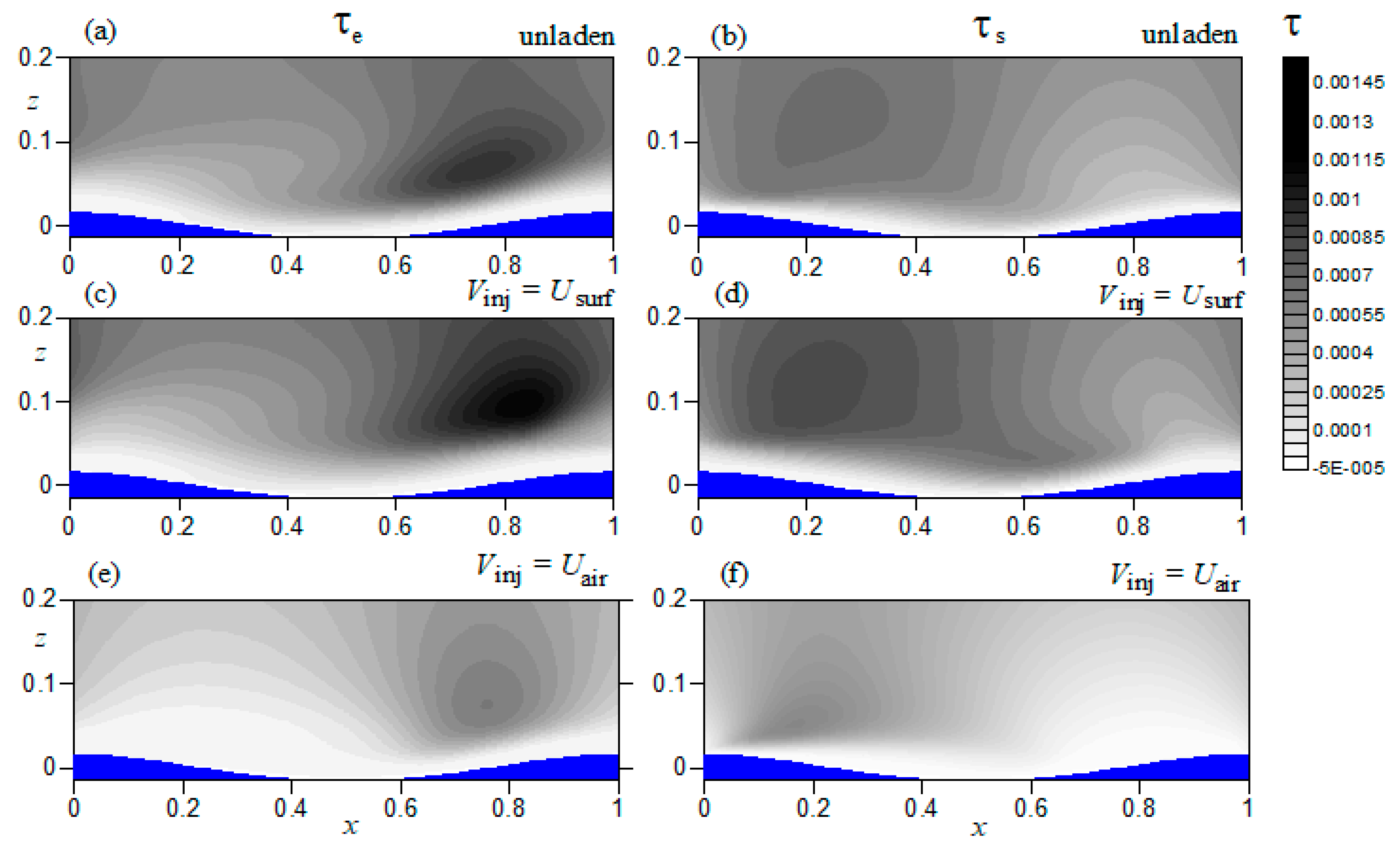
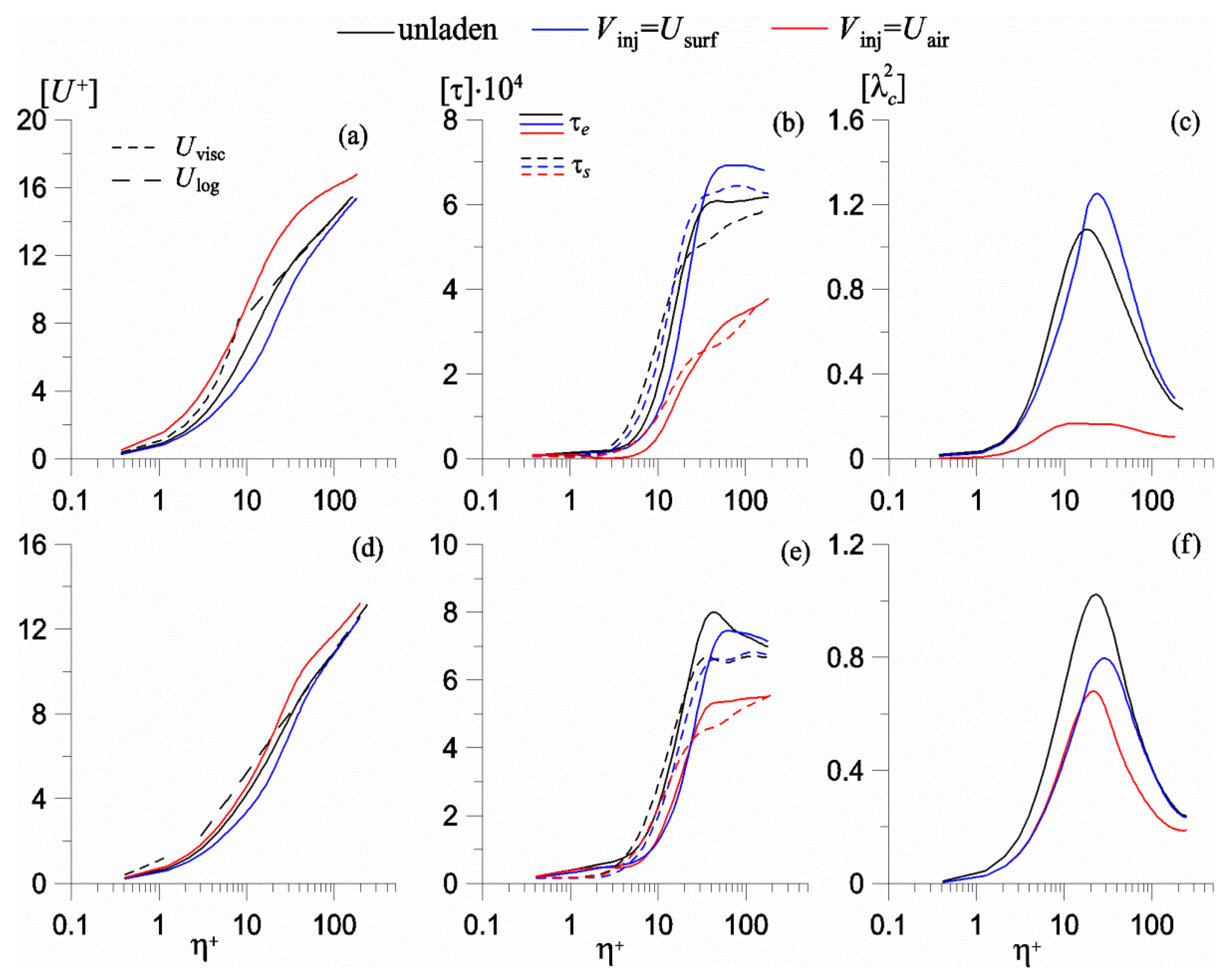
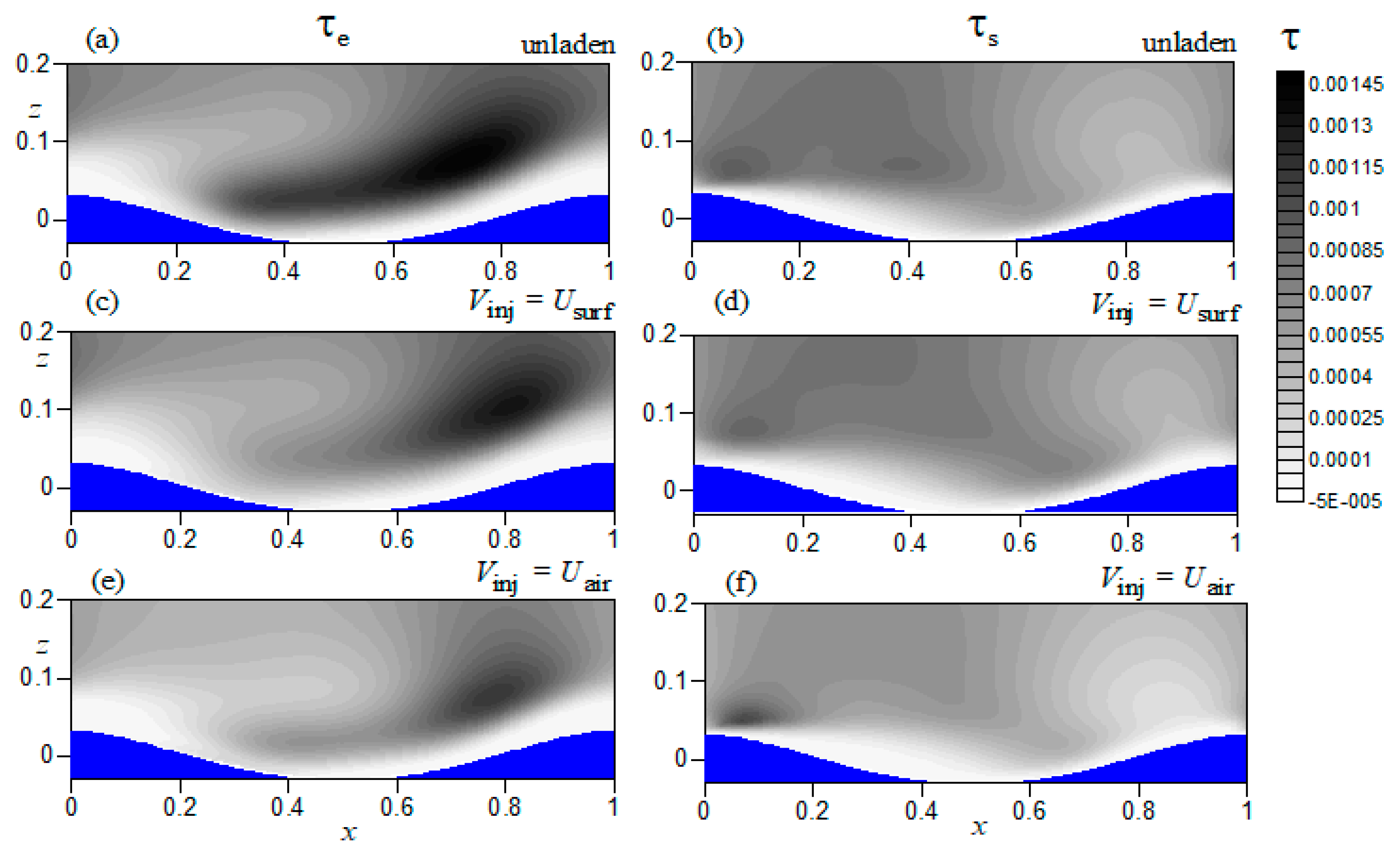
Sweep and ejections events are characterized by conditional correlations of x- and z- of the velocity fluctuation components (i.e., stresses) defined as [8]:
ejection   events :   τ e = U x U z ,   where   U x = U x U x <   0 ;   U z = U z U z >   0
sweep   events :   τ s = U x U z ,   where   U x >   0 ;   U z <   0 .
Vertical profiles of the stresses, [ τ e ] and [ τ s ] , are also evaluated according to Equation (27).

4. Results and Discussion

DNS was performed with the same bulk air-flow Reynolds number (Re = 15,000, Re = u λ / ν 500 , the friction air velocity u 0.03 U 0 ), dimensionless wave celerity c = 0.05 and two different wave slopes, ka = 0.1 and 0.2, both for the unladen and droplet-laden cases and different injection scenarios. Monodispersed droplets with diameter d = 200 µm and total number Nd = 3 × 10⁶ were considered. The dimensional time and length scales corresponding to the chosen flow parameters are 0.26 m and 0.3 s; the dimensionless gravity acceleration is g ≈ 0.08 cm/s2. The ratio of the dimensionless droplet size over the wall scale equals Re d / λ 0.4 , so the droplets can be treated as point particles.

4.1. Instantaneous Flow Fields

Figure 2, Figure 3 and Figure 4 present instantaneous distributions of the airflow vorticity modulus (in gray scale), ω , defined as:
ω = ( ω i ω i ) 1 / 2 , ω i = ε i j k U i x j .  
where summation over repeated indices is implied, and droplets respective distributions (symbols) in the central (x,z) and (y,z) planes and in (x,y) plane at the height η 0.04 above the water surface computed with wave steepness ka = 0.1 for unladen (Figure 2) and droplet-laden cases with two different injection scenarios ( V i n j = U s u r f , Figure 3, and V i n j = U a i r , Figure 4). As illustrated, in the droplet-free case (Figure 2), the instantaneous flow field exhibits numerous boundary layer separation points and occurrences of large-scale vortex structures (also known as “lambda”—vortices) observed also in previous DNS studies of droplet-free boundary layer flows over waved surfaces [7,8,9,27]. The comparison of the vorticity distributions in Figure 2, Figure 3 and Figure 4 shows that droplets injected with the air velocity are confined mostly in the near-surface (z < 0.1) layer and substantially reduce the intensity and quantity of large-scale structures in the droplet-laden air flow as compared to both the unladen-flow and V i n j = U s u r f cases. This impact of droplets on the carrier flow is similar to the effect of attenuation of large-scale vortices by solid particles observed in the vicinity of a flat, solid boundary [14,15]. In the case of droplets injected with the water surface velocity (Figure 4), the air turbulence vorticity attenuation is not so pronounced. The DNS results (not presented here) also show that the vorticity attenuation is also less significant for surface waves with steepness ka = 0.2.
The instantaneous fields in Figure 2, Figure 3 and Figure 4, as well as other characteristics of the flow, are similar to those obtained and discussed in the previous DNS study [12]. So, we refer the interested reader to that discussion, and below we mainly discuss the vortex structure and turbulent momentum modification by the droplets in terms of phase-averaged fields.

4.2. Phase-Averaged Fields

In order to quantify the impact of droplets on the air flow vortex structure and the air–water–surface momentum transfer, the phased-averaged profiles of the complex eigenvalue, λ c 2 , Equation (28), and stresses τ e and τ s due to sweep and ejections events, Equations (31) and (32), were evaluated. The results are shown in Figure 5, Figure 6 and Figure 7.
As Figure 5a illustrates, in the unladen-flow case, λ c 2 , which characterizes the swirling strength of vortices, is maximal in the near-surface layer (z < 0.1) above the upwind slope. As the surface roughness increases, the maximum is shifted towards the wave trough (Figure 5b). Droplets injected with water surface velocity ( V i n j = U s u r f ) increase λ c 2 by about 20% for ka = 0.1 (Figure 5c), and, similarly, reduce λ c 2 for ka = 0.2, as compared to the droplet-free case. On the other hand, droplets with V i n j = U a i r reduce λ c 2 to near-zero for ka = 0.1 (Figure 5e) and by about 50% for ka = 0.2 (Figure 5f).
Figure 6 and Figure 7 present distributions of phase-averaged stresses, τ e and τ s , Equations (31) and (32), obtained for the unladen and droplet-laden flow cases for surface wave steepness ka = 0.1 and 0.2. In the unladen case, the maximum of τ e is found above the up-wind wave slope (Figure 6a and Figure 7a), whereas the maximum of τ s is above the windward slope (Figure 6b and Figure 7b). These distributions of τ e and τ s indicate that, in the considered case of a “slow” surface wave (as compared to the wind), ejections are dominant at the up-wind slope, and sweeps are mostly found above the windward wave slope.
Distributions in Figure 6c,d show that droplets injected with water surface velocity increase both τ e and τ s by about 20% as compared to the unladen flow for ka = 0.1. On the other hand, droplets injected with the surrounding air velocity significantly reduce the stresses (Figure 7e,f). On the other hand, the impact by the droplets in the case ka = 0.2 is less pronounced. This is in accord with the instantaneous flow fields (Figure 3 and Figure 4), which show nearly similar intensity of the vortices in the V i n j = U s u r f case and a drastic reduction in the intensity and the number of the vortices in the airflow in the V i n j = U a i r case.
Figure 8 compares vertical profiles of mean air velocity, [ U + ] , stresses ( [ τ e ] and [ τ s ] ) and vortex swirling strength, [ λ c 2 ] , evaluated from the respective phased-averaged fields as described in Equations (26) and (27), for droplet-free and laden cases with different wave steepness and droplet injection scenarios. The mean air velocity in Figure 8a (ka = 0.1) and Figure 8d (ka = 0.2) is normalized with the friction velocity, u 0.03 U 0 , and the profiles, [ U + ] , are compared against the viscous asymptotics (in the viscous sublayer region, in a short dashed line) and the Monin–Obukhov (MO) self-similarity law in the logarithmic layer of MABL (in dashed line) [1,17]:
U v i s c = η + η ν u ,   U log = 2.5 ln ( η η 0 ) ,
where η 0 is the roughness length defined as a sum of the viscous length scale and the surface wave amplitude multiplied with a factor defined by a best fit for each considered wave steepness,
η 0 = 0.11 ν u + γ a
where γ = 0.028 for ka = 0.1, and γ = 0.07, for ka = 0.2. Figure 8a,d show that the unladen-flow mean velocity profile is well predicted by the MO theory, Equation (34). In the case ka = 0.1, droplets injected with the surface wave velocity ( V i n j = U s u r f , blue color) decelerate the air flow (7a,d), and increase both the stresses (8b,e), and the swirl (Figure 8a–c), whereas droplets injected with airflow velocity ( V i n j = U a i r ) accelerate the mean wind, reduce the stresses and the swirling strength.
On the other hand, for wave steepness ka = 0.2 (Figure 8d), the effects of acceleration/deceleration of the wind by the droplets are quantitatively less pronounced, as compared to the case ka = 0.1. The stresses and the swirl are also reduced significantly (by about 30%) by droplets with V i n j = U a i r as compared to the droplet-free flow (Figure 8e,f). However, for this wave steepness, ka = 0.2, the stresses are not enhanced by the droplets injected with the surface wave velocity ( V i n j = U s u r f ) as is observed in simulations with steepness ka = 0.1 (Figure 8b), whereas the swirling strength is reduced by about 30% as compared to the droplet-free flow (Figure 8f).

5. Conclusions

We have performed direct numerical simulation (DNS) of droplet-laden airflow over a waved water surface modeling the marine atmospheric boundary layer (MABL) carrying idealized spume sea-spray droplets. A Eulerian–Lagrangian approach is employed where full, 3D Navier–Stokes equations for the carrier air are solved in a Eulerian frame, and the trajectories of individual droplets are simultaneously tracked in a Lagrangian frame, taking into account the impact of the droplets on the carrier airflow. The droplets diameters are considered close to the typical size of spume droplets in the MABL (around 200 microns). The surface wave shape is prescribed and assumed to be unaffected by either droplets and/or air. Both instantaneous and phase-averaged flow fields, the Reynolds stresses, characterizing the sweeps and ejections events, and the eigenvalues of the local air-velocity gradient tensor are evaluated for two water surface roughness and two different droplet injection scenarios considered in DNS. The specific goal is to investigate the impact of the dispersed spray on MABL vortex structures and air–sea momentum transfer.
The DNS results show a strong dependence of the droplet-mediated modification of the airflow on the spume droplet velocity distribution at injection. Droplets injected with the surrounding air velocity effectively mitigate MABL vortex structures by reducing their swirling strength and suppress the momentum flux from air turbulence to water surface by weakening both ejections and sweeping events, and thus accelerating the mean flow as compared to the droplet-free MABL. On the other hand, droplets injected with the velocities of the Lagrangian particles of the water surface enhance both the swirling strength of MABL vortex structures and air-flow turbulent stresses and decelerate the mean wind. The results also show that these effects of droplet-mediated flow modification become less pronounced as the water surface roughness increases. This duplicity of the simulation results (as far as the droplet-mediated flow modification is concerned) assumes that more yet-unknown details of droplet injection mechanism are to be discovered and incorporated in the numerical code. This however depends on experimental (field and lab) efforts and is thus a subject for future research.

Author Contributions

Algorithm development, performing DNS, data analysis, writing—original draft preparation, O.A.D.; methodology, formal analysis, writing—review and editing, W.-T.T. All authors have read and agreed to the published version of the manuscript.

Funding

This work is supported by the Russian-Taiwanese Joint Research Project through the Russia RFBR Grant (No. 21-55-52005) and the Taiwan MOST Grant (MOST 110-2923-M-002-014 –MY3). OD is additionally supported by RFBR Grant (No. 20-05-00322), and by the Ministry of Education and Science of the Russian Federation (Task No. 0030-2022-0005).

Institutional Review Board Statement

Not applicable.

Informed Consent Statement

Not applicable.

Data Availability Statement

Not applicable.

Conflicts of Interest

The authors declare no conflict of interest.

References

  1. Phillips, O.M. The Dynamics of the Upper Ocean, 2nd ed.; Oxford University Press: Oxford, UK, 1975; pp. 1–196. [Google Scholar]
  2. Robinson, S.K. Coherent motions in the turbulent boundary layer. Annu. Rev. Fluid Mech. 1991, 23, 601–639. [Google Scholar] [CrossRef]
  3. Donelan, M.A.; Babanin, A.V.; Young, I.R.; Banner, M.L.; McCormick, C. Wave follower field measurements of the wind input spectral function. Part I. Measurements and calibrations. J. Atmos. Ocean. Technol. 2005, 22, 799–813. [Google Scholar] [CrossRef]
  4. Andreas, E.L.; Mahrt, L.; Vickers, D. An improved bulk air-sea surface flux algorithm, including spray transfer. Q. J. R. Meteorol. Soc. 2015, 141, 642–654. [Google Scholar] [CrossRef]
  5. Bortkovskii, R.S. Air-Sea Exchange of Heat and Moisture during Storms; D. Reidel: Dodrecht, The Netherlands, 1987; pp. 1–206. [Google Scholar]
  6. Richter, D.H.; Sullivan, P.P. Sea surface drag and the role of spray. Geophys. Res. Lett. 2013, 40, 656–660. [Google Scholar] [CrossRef] [Green Version]
  7. Sullivan, P.P.; McWilliams, J.C.; Moeng, C.-H. Simulation of turbulent flow over idealized water waves. J. Fluid Mech. 2000, 404, 47–85. [Google Scholar] [CrossRef] [Green Version]
  8. Yang, D.; Shen, L. Characteristics of coherent vortical structures in turbulent flows over progressive surface waves. Phys. Fluids 2009, 21, 125106. [Google Scholar] [CrossRef]
  9. Druzhinin, O.A.; Troitskaya, Y.I.; Zilitinkevich, S.S. Direct numerical simulation of a turbulent wind over a wavy water surface. J. Geophys. Res. 2012, 117, C00J05. [Google Scholar] [CrossRef]
  10. Druzhinin, O.; Troitskaya, Y.; Tsai, W.-t.; Chen, P.-C. The study of a turbulent air flow over capillary–gravity water surface waves by direct numerical simulation. Ocean Model. 2019, 140, 101407. [Google Scholar] [CrossRef]
  11. Chen, P.-c.; Tsai, W.-t.; Druzhinin, O.; Troitskaya, Y. The study of a turbulent air flow over capillary–gravity water surface waves: Characteristics of coherent vortical structures. Ocean Model. 2020, 150, 101621. [Google Scholar] [CrossRef]
  12. Druzhinin, O.A.; Troitskaya, Y.I.; Zilitinkevich, S.S. The study of droplet-laden turbulent air-flow over waved water surface by direct numerical simulation. J. Geophys. Res. Ocean. 2017, 122, 1789–1807. [Google Scholar] [CrossRef]
  13. Richter, D.H.; Dempsey, A.E.; Sullivan, P.P. Turbulent transport of spray droplets in the vicinity of moving surface waves. J. Phys Oceanogr. 2019, 49, 1789–1807. [Google Scholar] [CrossRef]
  14. Peng, T.; Richter, D. Sea spray and its Feedback effects: Assessing bulk algorithms of air–sea heat fluxes via direct numerical simulations. J. Phys. Oceanogr. 2019, 49, 1403–1421. [Google Scholar] [CrossRef]
  15. Dritselis, C.D.; Vlachos, N.S. Numerical study of educed coherent structures in the near-wall region of a particle-laden channel flow. Phys. Fluids 2008, 20, 055103. [Google Scholar] [CrossRef]
  16. Richter, D.H.; Sullivan, P.P. Modification of near-wall coherent structures by inertial particles. Phys. Fluids 2014, 26, 103304. [Google Scholar] [CrossRef] [Green Version]
  17. Powell, M.D.; Vickery, P.J.; Reinhold, T.A. Reduced drag coefficient for high wind speeds in tropical cyclones. Nature 2003, 422, 279–283. [Google Scholar] [CrossRef]
  18. Fairall, C.W.; Banner, M.L.; Peirson, W.L.; Asher, W.; Morrison, R.P. Investigation of the physical scaling of sea spray spume droplet production. J. Geophys. Res. 2009, 114, C10001. [Google Scholar] [CrossRef]
  19. Gent, P.R.; Taylor, P.A. A numerical model of the air flow above water waves. J. Fluid Mech. 1976, 77, 105–128. [Google Scholar] [CrossRef]
  20. Monin, A.S.; Yaglom, A. Statistical Fluid Mechanics; MIT Press: Cambridge, MA, USA, 1975; p. 874. [Google Scholar]
  21. Maxey, M.R.; Riley, J.J. Equation of motion for a small rigid sphere in a non-uniform flow. Phys. Fluids 1983, 26, 49–60. [Google Scholar] [CrossRef]
  22. Daitche, A. On the role of the history force for inertial particles in turbulence. J. Fluid Mech. 2015, 782, 567–593. [Google Scholar] [CrossRef] [Green Version]
  23. Fletcher, C.A.J. Computational Techniques for Fluid Dynamics, 2nd ed.; Springer: Berlin/Heidelberg, Germany, 1991; p. 493. [Google Scholar]
  24. Troitskaya, Y.; Kandaurov, A.; Ermakova, O.; Kozlov, D.; Sergeev, D.; Zilitinkevich, S. Bag-break-up fragmentation as the dominant mechanism of sea-spray production at high winds. Sci. Rep. 2017, 7, 1614. [Google Scholar] [CrossRef]
  25. Andreas, E.L.; Jones, K.F.; Fairall, C.W. Production velocity of sea spray droplets. J. Geophys. Res. 2010, 115, C12065. [Google Scholar] [CrossRef]
  26. Zhou, J.; Adrian, R.J.; Balachandar, S.; Kendall, T.M. Mechanisms for generating coherent packets of hairpin vortices in channel flow. J. Fluid Mech. 1999, 387, 353–396. [Google Scholar] [CrossRef]
  27. Moin, P.; Kim, J. The structure of the vorticity field in the turbulent channel flow: Part 1. Analysis of instantaneous fields and statistical correlations. J. Fluid Mech. 1985, 155, 441–464. [Google Scholar] [CrossRef] [Green Version]
Figure 1. Schematic of the problem: the upper panel shows the physical domain where (x, y, z) are Cartesian coordinates; a, λ, c are the surface wave amplitude, length and celerity; g is the acceleration due to gravity. The physical domain is transformed by mapping (1) into the computational domain (lower panel) with a flat bottom employing curvilinear coordinates (ξ, y, η) and a reference frame moving in the wave propagation direction with velocity c. Symbols show injected droplets (not to scale).
Jmse 10 00856 g001
Figure 2. Instantaneous distribution of the vorticity modus, ω, obtained in central (x,z) (a) and (y,z) (c) planes and in a near-surface (x,y) plane at η = 0.04 (b) in DNS with ka = 0.1 in the unladen flow case. Here and below in Figure 3 and Figure 4, only part of the total domain is shown in panels (a,b).
Jmse 10 00856 g002
Figure 3. The same as in Figure 2, but for the droplet-laden flow with V i n j = U s u r f . Droplets are shown by symbols (not to scale).
Jmse 10 00856 g003
Figure 4. The same as in Figure 3, but for the droplet-laden flow with V i n j = U a i r .
Jmse 10 00856 g004
Figure 5. Phase-averaged swirling strength, λ c 2 , obtained for different wave steepness (ka = 0.1, left and ka = 0.2, right) and droplet-free (panels a,b) and droplet laden flows with different injection scenario ( V i n j = U s u r f , (panels c,d), and V i n j = U a i r , panels e,f).
Jmse 10 00856 g005
Figure 6. Phase-averaged stresses, τ e and τ s (left and right), obtained for wave steepness ka = 0.1 in droplet-free (panels a,b) and droplet laden flows with different injection scenario ( V i n j = U s u r f , panels c,d, and V i n j = U a i r , panels e,f).
Jmse 10 00856 g006
Figure 7. The same as in Figure 6, but for wave steepness ka = 0.2.
Jmse 10 00856 g007
Figure 8. Profiles of mean velocity [ U + ] (panels a,d), stresses [ τ e , s ] (full and dashed line, respectively) (b,e) and swirling strength [ λ c 2 ] (c,f) obtained for droplet-free (black) and laden flows ( V i n j = U s u r f , blue, and V i n j = U a i r , red) with wave steepness ka = 0.1 (ac) and ka = 0.2 (df). The mean velocity profiles in panels (a,d) are compared against the viscous and logarithmic asymptotics, U v i s c and U log , Equation (34). η + = η ν / u is the normalized distance to water.
Jmse 10 00856 g008
Publisher’s Note: MDPI stays neutral with regard to jurisdictional claims in published maps and institutional affiliations.

