Calibration and Verification of a Hydrodynamic Model for a Narrow Estuary Receiving Submarine Groundwater Discharges

Abstract

This paper presents calibration and verification of the laterally averaged model for estuaries (LAMFE) for the Chassahowitzka River, a spring-fed estuary located on the Gulf coast of central Florida, USA. The river is a narrow and complex riverine system that receives submarine groundwater discharges (SGDs), which are difficult to measure. This study tried to make a reasonable estimate of some unquantified or missing SGD data with a trial-and-error approach in the model calibration process. The model was successfully calibrated against measured real-time data of water level, salinity, and temperature at three locations within the simulation domain from November 2012 to December 2015, before it was verified for the period from January 2016 to March 2017. Skill assessment of the model performance included visual comparisons and statistical quantifications of the difference between measured real-time data and model results. Both have shown that the LAMFE model performs well in simulating hydrodynamics, salinity transport, and thermal dynamics in the estuary. The good agreement of model results with field data suggests that the estimation of unquantified or missing SGDs in the spring-fed estuary is reasonable.

1. Introduction

Located on the Gulf Coast of the Florida peninsula, the Chassahowitzka River is a spring-fed estuary (Figure 1). The river is shallow and narrow and barely receives any surface water runoff from its 230 km² watershed. Hydrologic loadings to the Chassahowitzka River mainly come from its contributing groundwater field, or springshed, in the form of submarine groundwater discharges from a number of spring vents, which can be found at its headspring area and in several of its tributaries. The springshed is delineated based on the potentiometric contours in the region in a way similar to that used in the watershed delineation. Unlike a watershed, which generally has a stable shape and size, a springshed can vary slowly with time, because the potentiometric contours are affected by rainfall, which varies with time. For the spring flows entering the Chassahowitzka River estuary, the area of the springshed is estimated to be about 492 km², more than double the size of its watershed.

The Chassahowitzka River is a shallow and well/partially mixed estuary. Many marine species such as Common Snook (Centropomus undecimalis) and Florida manatees (Trichechus manatus latirostris) use the river as thermal refuges in winters, because the estuarine system receives a large and relatively stable rate of warm SGD with a temperature of about 23 °C. Protecting thermal habitats in the Chassahowitzka River is ecologically critical to the estuarine system and economically important to local communities. The region is well-known for manatee-related tourism, which attracts millions of visitors to the Gulf Coast of Florida. To protect this ecologically valuable springs/estuarine system, a minimum spring water flow rate was established [1] and recently re-evaluated by the Southwest Florida Water Management District [2].

Physical processes such as circulations, salinity transport processes, and thermal dynamics in the Chassahowitzka River estuary have never been thoroughly studied before and there exists very limited effort on hydrodynamic modeling of the estuary in literature. Dynamic Solutions [3] used the 3D model EDFC, or the Environmental Fluid Dynamics Code, developed by Hamrick [4] to simulate hydrodynamics in the Chassahowitzka River estuary. They discretize the riverine estuary with a typical grid size of 50 m by 80 m in the horizontal plane and four σ layers in the vertical direction. Due to the relatively coarse grids used in the simulation, their modeling study could not reasonably resolve the bathymetric variations in the estuarine system in many river segments, especially in the upstream narrow area as well as the tributaries and distributaries. The EDFC model for the Chassahowitzka River estuary was calibrated for a four-month period from November 2006 to February 2007 [3], basically only for the cold months of the year when the SGD entering the system was the lowest. Although the EFDC model was calibrated against measured real-time data of water elevation, salinity, and temperature at two stations, there was no verification of the model.

Similar to many other narrow riverine estuaries such as the lower Alafia River Estuary [5], Tanshui River estuary [6], as well as the lower Peace River and tidal Caloosahatchee River in the Charlotte Harbor estuarine system [7], the transversal variations of flow, salinity, and temperature in the Chassahowitzka River estuary are much smaller than those in the longitudinal and vertical directions due to its narrowness. As a result, circulations, as well as salinity and temperature distributions in the Chassahowitzka River, are generally vertically two-dimensional, a typical flow pattern for narrow estuaries [8,9,10]. The most suitable hydrodynamic model for the Chassahowitzka River is a laterally averaged (2DV) model such as the LAMFE model [11]. One advantage of a 2DV model in dealing with the complexity of the braided riverine system is that the wetting and drying phenomenon can be simulated automatically and accurately, simply because the river width is included in the governing equations as a variable (please see Section 3). The LAMFE model has another advantage over other hydrodynamic models such as the EFDC mode: It runs very fast and thus allows several years of simulation to be done in a couple of hours. The very short running time of the LAMFE model is not only due to a reduced dimension but also due to the use of an efficient semi-implicit scheme named the free-surface correction (FSC) method [11]. The FSC method is unconditionally stable with respect to gravity waves, wind and bottom shear stresses, and vertical eddy viscosity terms. While the EFDC model developed for the Chassahowitzka River could only be run with a time step of about 6 s or less, the LAMFE model developed for the Chassahowitzka River can be run with a time step of 75 s or longer, with a much finer resolution in both longitudinal and vertical directions than that used in the EFDC model [3]. The LAMFE model was applied to several narrow riverine systems in Florida, including the lower Hillsborough River [10], the lower Alafia River [5], etc. In all these applications, the Courant number used in the model runs was generally of the order of 15 or larger.

Since SGDs constitute a majority of the hydrologic loading to the Chassahowitzka River, a good quantification of SGDs for the estuarine system is important for a successful simulation of the Chassahowitzka River. Although a lot of flow data exist for the Chassahowitzka River, there are still plenty of missing SGDs, especially for some small spring vents. As a result, some of the SGD data had to be estimated based on data available for this modeling study. As discussed in Chen [12], most previous hydrodynamic modeling studies for estuarine and coastal waters did not include groundwater contributions. One reason is that the magnitude of groundwater discharge is usually much lower than river flows for most estuaries. Another reason is that SGDs are very difficult to quantify in a coastal environment. There are only very limited hydrodynamic modeling studies that included SGDs. Ganju et al. [13] estimated tidal and groundwater fluxes to West Falmouth Harbor, Massachusetts from measured velocity and salinity data and verified their flux estimates using the 3D model ROMS [14]. Chen [12] included SGDs in the hydrodynamic simulation for the Crystal River/Kings Bay system, another spring-fed estuary that is about 20 km north of the Chassahowitzka River. From measured real-time discharge data through two controlling cross-sections and tide data in Kings Bay, Chen [12] found that SGDs entering the Crystal River/Kings Bay are not only negatively proportional to tides in Kings Bay but also positively proportional to the first derivative of tides with respect to time.

This paper presents a modeling study of hydrodynamics, salinity transport processes, and thermal dynamics in the Chassahowitzka River using the LAMFE model, with the emphasis being placed on model calibration and verification. The model was calibrated for a 38-month period, from November 2012 to December 2015, while model verification was conducted for 15 months, from January 2016 to March 2017. The model calibration process included an estimation of SGDs from several spring vents where discharge data either are not available or contain many missing data points. Simulated water elevations, salinities, and temperatures were compared against real-time data measured at three fixed stations.

In the following, physical characteristics of the Chassahowitzka River estuary are provided in Section 2, which also includes some information about field data. Section 3 is a brief review of the laterally averaged hydrodynamic model LAMFE, while Section 4 presents the model setup and model calibration and verification, including visual comparisons of simulated water levels, salinities, temperatures, and discharges to real-time field data. In Section 5, the performance of the LAMFE model for the Chassahowitzka River estuary is assessed with a set of statistical measurements. The conclusions of this modeling study are summarized at the end of the paper in Section 6.

2. Physical Characteristics of the Estuary

The Chassahowitzka River estuary (Figure 1) originates in Citrus County in the State of Florida, USA, and flows to the Gulf of Mexico at Chassahowitzka Bay. The river is about 9 km long, with a mean depth of 0.9 m, or 3 feet [15]. The width of the Chassahowitzka River varies between about 30 m or less in the upstream portion of the river and over 550 m near its mouth. Figure 2 shows a map of the bathymetry data surveyed in the Chassahowitzka River estuary [16]. As can be seen from the figure, relatively deeper areas exist only in the downstream quarter of the main stem of the Chassahowitzka River, where the bottom elevation of the river is about −3.0 m, NAVD88 or lower, with several deep holes being −5 m, NAVD88 or deeper. In the most upstream 10% of the river, the river bottom is generally shallower than −1 m, NAVD88. There are several shoals in the upstream reach, where most of the bottom is shallower than −0.5 m, NAVD88, except for areas in the navigation channel. All the tributaries and distributaries are very shallow, with the bottom elevation generally being higher than −1 m, NAVD 88.

The Chassahowitzka River flows through a Coastal Swamps area with poorly drained and saturated organic soils that overlie limestones of the Upper Florida Aquifer (UFA). Since most of the wetland of the Chassahowitzka River is self-percolating, it barely contributes any quantifiable surface water runoff to the river. Surface water entering the estuary is negligible in comparison with groundwater discharges from the UFA. SGDs are mainly out of numerous spring vents located in the headspring area and in several of its tributaries. The estimated contributing springshed varies slowly with time and has an average of about 492 km².

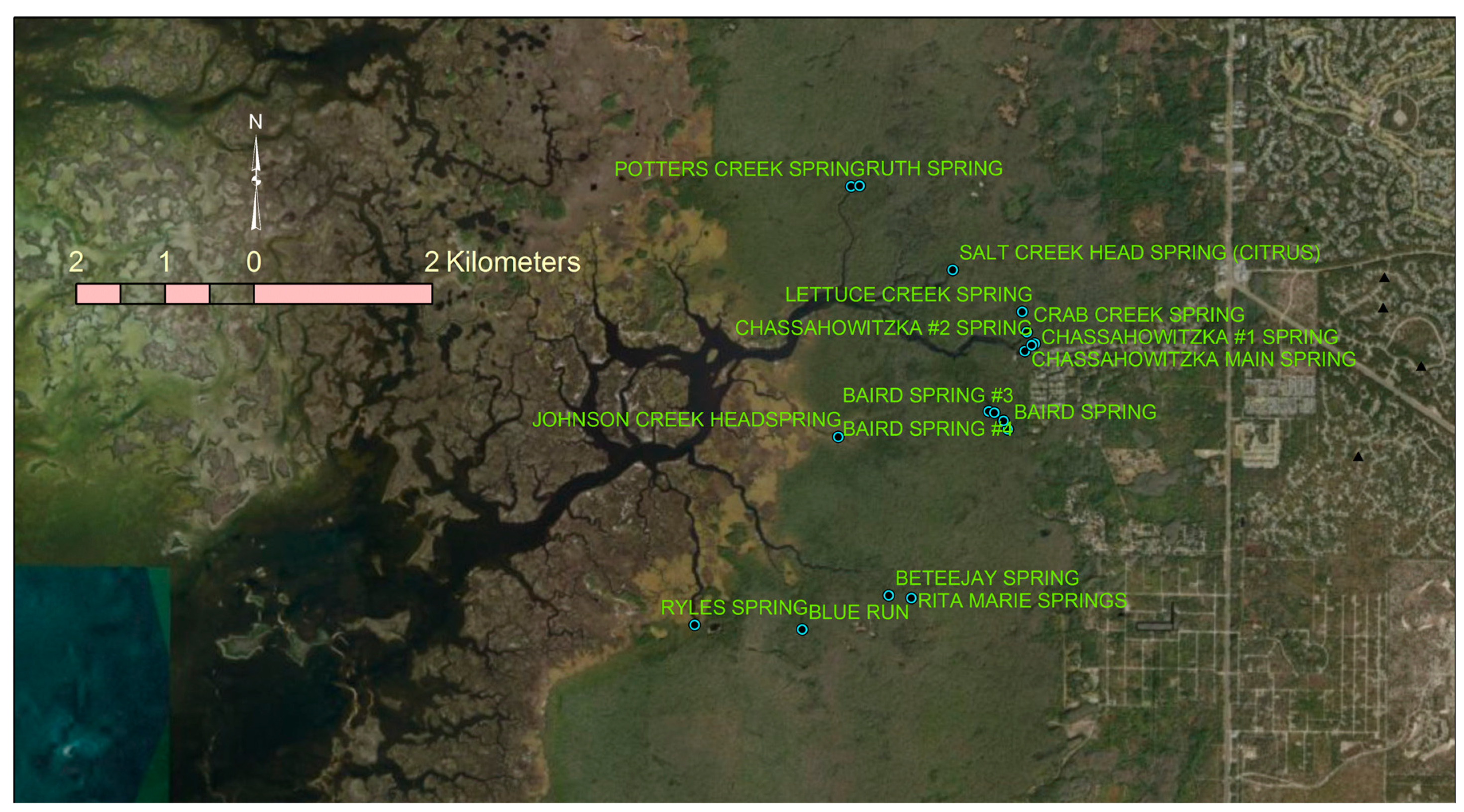
Figure 3 shows the locations of the spring vents that discharge groundwater flows to the Chassahowitzka River. The Chassahowitzka Main Spring, Chassahowitzka #1, Chassahowitzka #2, and several unnamed springs upstream of the headwaters for the Chassahowitzka River [17]. Many spring flows discharging to the Chassahowitzka tributaries are insignificant, except for the Crab Creek spring, the Potters Creek spring (including Ruth spring), Baird Creek springs, and those flowing to the Crawford Creek, possibly from the Beteejay spring and Rita Marie springs. Please see Figure 1 for locations of the Crab, Potters, Baird, and Crawford creeks.

Although the Chassahowitzka Main, Chassahowitzka #1, and Chassahowitzka #2 are considered the headwaters of the river, there exists a channel network upstream of the headspring area, connecting to the Chassahowitzka River and allowing for residents living along the channels to get access to the river. Although surface water runoff to this channel network is negligible, there are some relatively small SGDs entering the channels, which are eventually gauged at a United States Geological Survey (USGS) station just above the Crab Creek confluence in the Chassahowitzka River, namely the USGS Chassahowitzka River near Homosassa (CRH) station, using an acoustic Doppler current profiler (ADCP). In addition to these small SGDs, there is also tidal flow, which comes from and enters the channel network but contributes no net flow for the Chassahowitzka River.

Besides the CRH station, real-time discharge was also gauged using an ADCP at the USGS Chassahowitzka River near Chassahowitzka (CRC) station, which is located about 3.5 km downstream of the CRH station. Figure 4 shows discharge data through the cross-sections at the CRH and CRC stations during a 60-day period, from 13 June 2015 to 11 August 2015. Gauged discharge data for their periods of record can be found in Chen [18]. In Figure 4, a positive discharge flows in the downstream direction, while a negative discharge flows in the upstream direction of the river. From Figure 4, one can see that the discharge gauged at the CRC station varied roughly from −36 m³/s to 24 m³/s most of the time. At the CRH station, the discharge varied between about −1 m³/s to about 3 m³/s, which was more than one order of magnitude smaller than the tidal variability of the discharge at the CRC station, as the former has a much smaller tidal prism than the latter. During the first three days of August 2015, an area of low pressure in the eastern Gulf of Mexico caused a storm event in the region and brought heavy rains across portions of Central Florida. As a result, discharge from 1 August to 3 August had a significant increase at the CRC station, varying from about −145 m³/s to about 75 m³/s. Long-term averages of the discharges are 2.66 m³/s and 1.74 m³/s through the cross-sections at the CRC and CRH stations, respectively. In other words, the river segment between the two cross-sections receives about 0.92 m³/s of SGD.

Like some other estuaries along the Gulf Coast of Florida, the Chassahowitzka River estuary is under the action of microtidal forces, which are primarily semidiurnal. Tidal data were collected by the USGS at four fixed stations in the Chassahowitzka River, at which specific conductance and temperature data were also collected. In addition to the CRH and CRC stations, there are two other USGS real-time CDT stations in the estuary, namely the USGS Chassahowitzka River at Dog Island near Chassahowitzka (CRD) and the USGS Chassahowitzka River at Mouth near Chassahowitzka (CRM) stations, both at the downstream portion of the river. General information about the four USGS CDT stations is provided in

Table 1. General information about the USGS CDT data collection stations in the Chassahowitzka River.

Station Name	CRH	CRC	CRD	CRM
Station #	2310650	2310663	2310673	2310674
Longitude	82 34 38.38 W	82 36 22.35 W	82 37 28.35 W	82 38 20.35 W
Latitude	28 42 55.71 N	28 42 54.95 N	28 42 09.95 N	28 41 40.95 N
Available since	11 October 2007	1 May 2003	12 September 2005	11 October 2005
Datum	NGVD29	−0.71 ft, NAVD88	NAVD88	NAVD88
Sensor elev. (ft, NAVD88)	−2.42	−4.32	−2.06	−2.80
			−4.21	−6.25

, including station name, station number, longitude, latitude, starting date of the data collection, datum, and sensor elevations for conductance and temperature. The locations of the four stations are marked with solid green triangles in Figure 1.

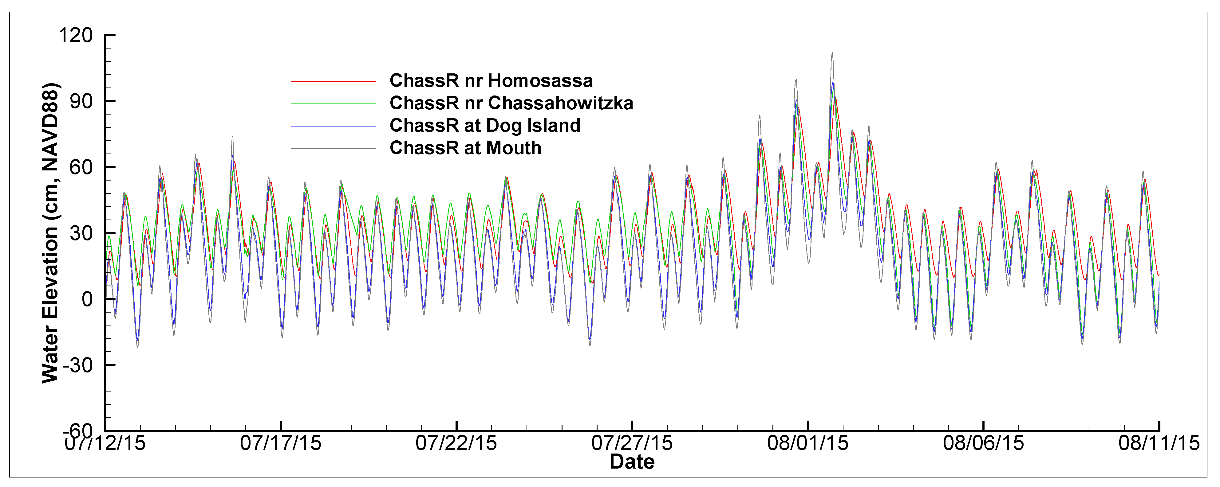
Figure 5 shows water elevations measured at the CRH, CRC, CRD, and CDM stations in the Chassahowitzka River. For a clearer presentation, the figure only includes 30 days of tides (the second half of the 60-day discharge graph is shown in Figure 4). Nevertheless, it shows the basic characteristics of tides in the estuary. Diurnal and semidiurnal tidal variabilities can be seen from the figure, with the semidiurnal being more dominant. During neap tides, the water level variation is generally in the order of 40 cm. However, during spring tides, the water level can vary 90 cm, from about −20 cm, NAVD88 to almost 70 cm, NAVD88. During the storm event in early August, the water level reached over 100 cm, NAVD88. The existence of the shoals in the upstream portion of the river reflects tidal waves and causes a damming effect at the CRH station, where low tides are generally much higher than those at the other three stations.

Alongside the tidal force, barotropic and relatively weak baroclinic forces also affect hydrodynamic and transport processes in the Chassahowitzka River estuary, though their effects are generally lower than that of the tides. Salinity and temperature data obtained from the CDT measurement at the four USGS real-time stations show that the most upstream station (CRH) retains characteristics of the SGD out of the spring vents in the headspring area, with a relatively stable temperature and a salinity lower than 2.5 psu most of the time. Water temperatures in the two downstream stations (CRD and CRM) exhibit typical estuary characteristics, with a small diurnal variability but a large seasonable variability. The mouth of the Chassahowitzka River is located near the center of the southern half of the Florida Big Bend Coast, an area roughly from the mouth of the Suwannee River near Cedar Key, Florida to the mouth of the Anclote River near Tarpon Springs, Florida. The water of the Florida Big Bend Coast is generally shallower than 2 m and has an estimated area of about 2900 km² [19]. As a relatively small coastal waterbody, the Florida Big Bend Coast receives flows from several large watersheds (e.g., the Suwannee River and Withlacoochee River) and springsheds of first magnitude spring systems (e.g., Crystal, Homosassa, Chassahowitzka, and Weeki Watchee Rivers.) As a result, salinity along the Florida Big Bend Coast is generally low [19]. At the mouth of the Chassahowitzka River (CRM), salinity can be lower than 5 psu during the wet season (mainly summer months and early fall) and the highest salinity during the dry season (April–June) barely reaches 26 psu or above. There are some salinity and temperature stratifications in the estuary, but the stratification level is generally low.

The climatology in the Chassahowitzka River region has distinct winter and summer patterns. During the winter months, frequent frontal incursions and extratropical cyclones can occur and produce large shifts in wind speed and wind direction in response to rapidly changing atmospheric pressure and thermal gradients. The summer months are generally characterized by light and variable winds originating from the northeast trade wind circulation. Due to the strong differential heating of the land and adjacent waters along the coast, sea/land breezes are typical for the Florida peninsula during summer days. During the hurricane season (generally from June to November), tropical storms can occasionally move to the area, causing intense modifications to the meteorological conditions of the region.

More details on the CDT data measured in the Chassahowitzka River as well as meteorological data such as wind, air temperature, air humidity, solar radiation, and rainfall collected in the region are reported and discussed in Chen [18].

3. Laterally Averaged Hydrodynamic Model

As a narrow riverine system, circulation patterns and salinity and temperature distributions in the Chassahowitzka River vary primarily in the vertical and longitudinal directions. This study used the laterally averaged LAMFE [11] for the simulation of hydrodynamics, salinity transport processes, and thermal dynamics in the Chassahowitzka River. This section provides a brief overview of the LAMFE model.

The model uses the hydrostatic pressure assumption and solves the following laterally averaged governing equations [20,21]:

$$\frac{\partial ub}{\partial x}+\frac{\partial wb}{\partial z}=v$$

(1)

$$\frac{\partial u}{\partial t}+u\frac{\partial u}{\partial x}+w\frac{\partial u}{\partial z}=-\frac{{\tau }_{wx}}{{\rho }_{0}b}-g\frac{\partial \eta }{\partial x}-\frac{g}{{\rho }_0}{{\displaystyle \int }}_z^{\eta }\frac{\partial \rho }{\partial x}d\zeta +\frac{1}{b}\frac{\partial }{\partial x}\left(b{A}_h\frac{\partial u}{\partial x}\right)+\frac{1}{b}\frac{\partial }{\partial z}\left(b{A}_v\frac{\partial u}{\partial z}\right)$$

(2)

$$b\frac{\partial c}{\partial t}+\frac{\partial ubc}{\partial x}+\frac{\partial wbc}{\partial z}=\frac{\partial }{\partial z}\left(b{B}_h\frac{\partial c}{\partial x}\right)+\frac{\partial }{\partial z}\left(b{B}_v\frac{\partial c}{\partial z}\right)+v{c}_t$$

(3)

where x is the horizontal coordinate in the longitudinal direction (along the river/estuary); z is the vertical coordinate; t is time; c is concentration; u and w represent velocities in x- and z-directions, respectively; v is the velocity for lateral input (direct runoff, tributary, etc.); b is the width of the estuary (a function of x and z); ρ, g, and η denote density, gravitational acceleration, and the free surface elevation, respectively; ${\tau }_{wx}$ represents frictions at side walls (=ρC_wu[u² + w²]^1/2, where C_w is a frictional coefficient for side walls); A_h and A_v are eddy viscosities in the x- and z-directions, respectively; B_h and B_v are horizontal and vertical eddy diffusivities, respectively; and c_t represents the concentration in lateral input.

The equation for the free surface is obtained by integrating Equation (1) over the water depth

$$b_{\eta }\frac{\partial \eta }{\partial t}=-\frac{\partial }{\partial x}{{\displaystyle \int }}_{h_0}^{\eta }ubdz+{{\displaystyle \int }}_{h_0}^{\eta }vdz+r{b}_{\eta }$$

(4)

where h₀ is the bottom elevation; $b_{\eta }$ is the width of the river/estuary at the free surface; and r is the net rain intensity (rainfall minus evaporation).

In the LAMFE model, a Cartesian grid system is used with a staggered arrangement of model variables: surface elevation is computed at the center of the horizontal grid, and 2D scalar variables (e.g., pressure, concentration, and density) are calculated at the cell center; velocity components u- and w-velocities are calculated at the centers of the right and top faces of the cell, respectively. The Sub-Grid Scale model of Smagorinsky [22] was used to calculate horizontal eddy viscosity (A_h) and diffusivity (B_h). The LAMFE model provides several options for estimating vertical eddy viscosity (A_v) and diffusivity (B_v), including a simplified second-order closure model and a turbulent kinetic energy (TKE) model [23] that is similar to that of [24].

The solver of the LAMFE model uses a semi-implicit scheme named the FSC method, which involves a predictor-corrector approach. In the predictor step, the model treats the pressure gradient term and the convection terms explicitly but the vertical eddy viscosity terms and bottom and sidewall frictions implicitly. An intermediate velocity field is solved before it is used in Equation (4) to compute an intermediate free surface. The final free surface is obtained by adjusting the intermediate free surface with a free-surface correction, which is solved from an equation of the FSC. The equation of FSC is derived from a velocity field obtained with the semi-implicit treatment of the hydrostatic pressure term in the momentum equation. After the final free surface is found, the final velocity field is calculated by adjusting the intermediate velocity field using the FSC. The method is unconditionally stable with respect to gravity waves, bottom and wall frictions, and the vertical eddy viscosity term. In practical applications, it generally allows the model to run with a Courant number larger than 10. Details on the FSC method and its properties can be found in Chen [11]. Although the z-coordinate is used in the model without any transformation, the model can fit the bottom variation by using a piecewise linear bottom [10]. The resulting grid cells are hybrid, and their side views include regular Cartesian grid cells and multi-face cells that are cut with a piecewise linear bottom. Details on the use of the piecewise linear bottom to fit the bed variation in LAMFE are described in Chen [10].

From Equations (1)–(4), one can see that the river width (b) is included in the governing equations. As b at a fixed cross-section varies with z, the wetting/drying phenomenon is automatically simulated in the LAMFE model. No special treatments or any assumptions are needed to handle this phenomenon. Even when the cross-section involves a wide flood plain, the conveyance of the flow by the flood plain can be correctly considered in the model, provided that accurate bathymetry/topography data for the flood plain are available.

4. Model Simulations

4.1. Model Setup

The Chassahowitzka River system was discretized with 348 grids along the river’s main stem and its 19 branches, with a horizontal spacing of the grids varying between 10 m to 370 m. Figure 6 shows cross-sections that form the 348 LAMFE grids along the main stem of the Chassahowitzka River and its branches. The water body was discretized with 15 layers between elevations −5.1 m, NAVD88 and 3.3 m, NAVD88, with the layer thickness varying from 0.3 m to 1.2 m. With this discretization, major physical characteristics of the estuary can be reasonably resolved in the LAMFE model.

Based on the availability of measured data which were used to drive the model, a 52-month period between 18 November 2012 and 28 March 2017 was chosen for model calibration and verification. The period prior to 1 January 2016 was for model calibration, while the period between 1 January 2016–28 March 2017 was for model verification. A variable time step (Δt) was used in model runs, with Δt = 75 sec being used more than 99% of the time of the 52-month simulation period.

Input data used for boundary conditions to drive the model include measured data of water level, salinity, and temperature at the downstream open boundary (the CRM station), meteorological data collected at local weather stations, and SGDs entering the estuarine system. The meteorological data were used to calculate wind shear stresses acting on the free surface and the heat exchange through the air-water interface. SGDs were added to the simulation domain at the locations marked with orange arrows shown in Figure 6.

While available data are good enough to specify boundary conditions at the downstream open boundary and at the free surface, there is not enough data to quantify all the SGDs for the estuary. The only available real-time discharge data that are continuously collected for a long period of time and can be used as boundary conditions in this study are those measured at the CRH station (Figure 1) since 8 October 2012. Measured discharge through the cross-section of this station includes both SGDs upstream of it and the tidal flow through the cross-section. The net flow, which represents all SGDs upstream of the cross-section, can be calculated by taking away the tidal flow. Since the upstream portion of the CRH station is a relatively small area, any spatial variations of tides in the area are negligible and temporal variations of tides can be assumed to be the same as those at the measurement station. As such, the tidal flow can be approximated as follows

$$q_t=-A\frac{\partial \eta }{\partial t}$$

(5)

where $q_t$ is the tidal flow, with the positive flow pointing toward downstream, $\eta$ is measured water elevation, $t$ is time, and $A$ is the surface water area upstream of the cross-section. The tidal flow was specified at the upstream cross-section of the main stem of the Chassahowitzka River, while the net flow through the cross-section was added to the bottom layer of the most upstream grid.

There are only very limited discharge data for other SGDs entering the tributaries, including those of the Crab, Baird, Potters, and Crawford Creeks (see the orange arrows in Figure 6). Available discharges measured in these tributaries were mainly short-term and collected manually within only a few hours (generally less than 6 h). These data do not contain any continuous recordings that allow for a comprehensive analysis of the tidal effect on the SGD. The best way to estimate SGDs from spring vents in these tributaries was to assume that the effects of groundwater level and tides on SGDs in the tributaries are similar to these on SGDs gauged at the CRH station. As a result, it is reasonable to assume that tributary SGDs are proportional to those at the CRH station. This assumption may not be true over a short time scale (hours) as tides may have some time lags or leads for different locations but should be proper over a time scale of daily or longer. With this assumption, one can partition the total SGD entering the river segment between the CRC and CRH stations among the Crab, Baird, and Potters Creeks. After several trials and errors during model calibration, it was found that Crab, Baird, and Potters Creek respectively contribute about 64%, 7%, and 27% of the total SGD entering this river segment. The remaining 2% is from one or more unidentified sources within this river segment. As mentioned before, the river segment between the CRC and CRH stations receives roughly 0.92 cm³/s SGD in terms of the long-term average, representing about 53% of the long-term SGD through the cross-section at CRH. Based on the limited SGDs measured for Crab, Baird, and Potters creeks and several previous studies [3] and field measurements [25,26], it was found that the ratio of SGD received for the segment between the CRC and CRH stations over the gauged net flow through the cross-section at CRH varied in a range of 0.53–1.10, with a mean of about 0.83. In the model calibration process, this mean ratio of 0.83 was used to estimate the total SGD entering the river segment. As such, SGDs for Crab, Baird, and Potters Creeks are estimated as about 53.0%, 5.8%, and 22.4% of that through the cross-section of the CRH station. For the Crawford, Creek, it was estimated to be about 22.5% of the SGD gauged at the CRH station.

Due to the lack of direct measurements of salinity in the spring vents, salinity in SGD was unknown. This piece of information is needed as the boundary condition for the LAMFE model. To obtain a reasonable estimate of salinities in all SGDs, this study used a trial-and-error approach. Based on measured salinity at the CRH station and other available salinity data measured in the Chassahowitzka River system, numerous salinity estimates were tested in model runs. After careful analyses of simulated salinity results for all salinity estimates for SGDs and some limited salinity and temperature measurements in spring vents in Kings Bay, which is another estuary receiving SGDs in the region and <20 km north of the Chassahowitzka River, it was found that the following set of salinity estimate produces the best and most reasonable model results:

$$s_{cm}=min\left(max\left(s_0/1.025,0.5\right),5.0\right)$$

(6)

$$s_{cc}=s_{br}=s_{pc}=max\left(s_{cm}+0.25, 2.0\right)$$

(7)

$$s_{cf}=0.95$$

(8)

$$s_r=max\left(s_{cm}+0.25,2.0\right)+1.0$$

(9)

where $s_0$ represents measured salinity at the CRH station; $s_{cm}$ is the estimated SGD salinity in the headwaters; $s_{cc}$, $s_{br}$, $s_{pc}$, $s_r$, and $s_{cf}$ are estimated salinities in SGDs for the Crab, Baird, Potters Creeks, and Crawford Creeks, respectively; and $s_r$ is estimated salinity for the unidentified SGD source.

Similarly, information about temperatures in spring vents is also needed as the boundary condition for the LAMFE model. Generally, SGD temperature is stable and contains a very small tidal variation. From temperature data collected in spring vents in Kings Bay [12], it was found that spring water is slightly colder in winter than in other seasons. This kind of seasonal variability existed in the temperature data measured at the CRH station and is expected to exist in temperature from all the SGDs in the Chassahowitzka River system. After a trial-and-error process, this study used a combination of measured temperature and a constant temperature value as the estimate of water temperature in all spring vents in the Chassahowitzka River system:

$$T_{SGD}=\alpha T_{cm}+\left(1-\alpha \right)T_0$$

(10)

where $T_{SGD}$ is the estimated temperature in SGD; $T_{cm}$ is the measured temperature at the CRH station; $T_0$ is a constant value of 23.5 °C; and $\alpha$ is a model parameter and was determined to be 0.7 during the model calibration process. $T_0$ is obtained by examining the available temperature data measured inside all the spring vents in the region. $T_0$ is found to be very close to the mean of these temperature data.

4.2. Model Calibration and Verification

The LAMFE model was calibrated using measured real-time data of water level, salinity, and temperature at the CRH, CRC, and CRD stations. A series of adjustments of model parameters within certain allowable ranges was made to obtain the best match of simulated water levels, salinities, and temperatures with measured data in the field. Only a few input parameters had to be tuned in the calibration process, including the bottom roughness, ambient vertical eddy viscosity, and diffusivity, in addition to the trails and errors of salinity and temperature in spring discharges.

Model runs indicate that the most sensitive model parameter to simulated water levels in the upstream portion of the Chassahowitzka River is the bottom roughness. The existence of the shoals in the upstream area not only creates a damming effect in the upstream segment of the shoals but also increases the bottom roughness in the area, which causes more bottom frictions to the flow.

The most sensitive model parameter to simulated salinities is the turbulence mixing. As pointed out in Chen [27], the vertical mixing process plays a very important role in simulating salinity distributions in narrow estuaries that are under the action of microtidal forces. This study used the TKE closure model of Chen [23] to calculate the eddy viscosity and diffusivity in the vertical direction. To this end, the vertical ambient eddy viscosity and diffusivity also need to be properly chosen. In the model simulation, the ambient eddy viscosity was set as 1.0 cm²/s, while the ambient eddy diffusivity used was 0.2 cm²/s.

For temperature simulation, the most sensitive model parameter is the light attenuation coefficient. While the water temperature in the upstream area is dominated by the SGD temperature, it is affected by the light attenuation more significantly in the middle and downstream areas, as the heat transport in the vertical direction becomes more important.

Figure 7, Figure 8, Figure 9 and Figure 10 present comparisons of model results of water level, salinity, temperature, and discharge with measured field data at the three measurement stations in the Chassahowitzka River. In these figures, red lines are model results, while dashed blue lines are measured data. For simplicity and clarity, only 60 days (19 March 2013–18 May 2013) of simulated and measured water elevations are shown in Figure 7. For the same reason, only 40 days (8 April 2013–18 May 2013) of comparisons of simulated and measured salinities, temperatures, and discharges are presented in Figure 8, Figure 9 and Figure 10, respectively. The choice of these 60-day or 40-day periods is arbitrary. Comparisons of model results with real-time field data during other time periods are similar, with some having a slightly better match and some a slightly worse match. Plots showing visual comparisons of model results with field data of water level, salinity, and temperature during other time periods can be found in Chen [18].

As can be seen in Figure 7 and Figure 10, simulated water elevations at all three USGS stations and simulated discharge at the CRC station agree very well with the measured data. Simulated water levels at the three USGS stations have the same long-term and short-term variations as measured data. The damming effect caused by the shoals in the upstream reach of the river is correctly modeled in the simulated water elevations at the CRH station, matching the same phenomenon seen in the real-time data at the station. Simulated discharge at the CRC station generally matches measured discharge very well, except for some misses of negative peaks. Simulated discharges during the neap and spring tides have almost the same variabilities.

Modeled salinity and temperature results also have good agreement with field data (Figure 8 and Figure 9), with similar long-term and short-term variations. Due to the uncertainties included in the input data that drive salinity and temperature simulations, it is expected that the match between model results and data for salinity or temperature is not as good as that for water level simulation. Nevertheless, simulated salinity and temperature results are satisfactorily well-matched with measured real-time data. More details about comparisons of model results with field are presented in the next section, where skill assessment for the model is described.

With the LAMFE model being well-calibrated and verified, it was used to study the effects of SGD on salinity habitats such as water volumes, bottom areas, and shoreline lengths for various salinity ranges in the Chassahowitzka River estuary. Effects of SGD on thermal habitats for Florida manatees and Common Snook were also studied. As a detailed description and discussion of the effects of the SGD reduction on salinity and thermal habitats are beyond the scope of this article, only some major findings are included here. More information can be found in Chen [18] and at the website https://www.swfwmd.state.fl.us/projects/mfl/documents-and-reports (accessed on 1 June 2022).

It was found that salinity volume is generally more sensitive to the SGD reduction than salinity bottom area, which is more sensitive to the SGD reduction than salinity shoreline length. The acute condition for manatees (water volume with temperature ≥ 15 °C on a temporal scale of 4 h) is more sensitive than the chronic condition for manatees (water volume with temperature ≥ 20 °C on a temporal scale of 72 h) to the SGD reduction in the Chassahowitzka River. The most sensitive Common Snook thermal habitat is ≥15 °C water volume during a single cold day. With an 8.47% reduction of the SGD, the daily ≥ 15 °C water volume could drop 15%.

5. Model Performance Metrics

The performance of the LAMFE model for the Chassahowitzka River is assessed quantitatively with several statistics, including the mean error (ME), mean absolute error (MAE), root-mean-square error (RMSE), normalized root-mean-square error (NRMSE), the coefficient of determination (R²), and a skill assessment parameter introduced by Willmott [28]. The Willmott skill assessment parameter was used by Warner et al. [29] to assess the performance of a hydrodynamic model for the Hudson River estuary. It also was used by the author to examine the performances of hydrodynamic models applied to estuarine systems, including an unstructured 3D model for Crystal River/Kings Bay [12].

The Willmott skill assessment parameter takes the following form

$$S_k=1-\frac{\sum {\left(y^M-y^D\right)}^2}{\sum {\left(\left|y^M-\overline{y^D}\right|+\left|y^D-\overline{y^D}\right|\right)}^2}$$

(11)

where $S_k$ is the skill assessment parameter (or simply the skill); $y^M$ and $y^D$ represent simulated and measured variables (water level, salinity, etc.); and $\overline{y^D}$ is the expectation of $y^D$. $S_k$ in the above equation varies between 0 and 1, with one being a perfect agreement and zero being a complete disagreement between simulated results and measured data.

Mean errors, mean absolute errors, root-mean-square errors, normalized root-mean-square errors, coefficients of determination, and skills for simulated water elevations, salinities, and temperatures are listed in

Table 2. MEs, MAEs, RMSEs, NRMSEs, R² values, and skills for simulated water levels (cm) in comparison with real-time field data measured at the CRH, CRC, and CRD stations during the calibration period, the verification period, and the entire simulation period.

Station	ME	MAE	RMSE	NRMSE	R2	Skill
	Calibration Period
CRH	−5.201	7.236	8.867	0.083	0.816	0.919
CRC	−3.840	6.648	8.524	0.051	0.924	0.973
CRD	−1.688	4.966	6.121	0.034	0.954	0.986
Overall	−3.612	6.307	7.959	0.044	0.918	0.972
	Verification Period
CRH	−2.821	6.346	7.931	0.043	0.844	0.952
CRC	−2.394	5.802	7.947	0.043	0.923	0.977
CRD	−0.958	4.590	5.807	0.030	0.958	0.989
Overall	−2.132	5.648	7.383	0.030	0.921	0.978
	Entire Simulation (Calibration & Verification) Period
CRH	−4.531	6.986	8.614	0.047	0.817	0.931
CRC	−3.442	6.416	8.369	0.046	0.923	0.974
CRD	−1.506	4.873	6.044	0.031	0.955	0.987
Overall	−3.214	6.13	7.808	0.031	0.918	0.973

,

Table 3. MEs, MAEs, RMSEs, NRMSEs, R² values, and skills for simulated salinities (psu) in comparison with real-time field data measured at the CRH, CRC, and CRD stations during the calibration period, the verification period, and the entire simulation period.

Salinity (psu)	ME	MAE	RMSE	NRMSE	R2	Skill
	Calibration Period
CRH	0.011	0.285	0.412	0.087	0.833	0.929
CRC	0.314	1.168	1.581	0.081	0.654	0.893
CRD (Top)	−0.320	1.203	1.537	0.068	0.792	0.930
CRD (Bottom)	0.015	1.239	1.581	0.071	0.766	0.929
Overall	0.007	0.967	1.367	0.057	0.889	0.970
	Verification Period
CRH	0.042	0.330	0.509	0.033	0.735	0.890
CRC	0.062	1.468	1.988	0.106	0.620	0.883
CRD (Top)	−0.534	1.383	1.778	0.086	0.757	0.907
CRD (Bottom)	−0.220	1.401	1.780	0.099	0.730	0.907
Overall	−0.160	1.138	1.617	0.077	0.887	0.967
	Entire Simulation (Calibration & Verification) Period
CRH	0.021	0.299	0.443	0.029	0.801	0.918
CRC	0.239	1.257	1.712	0.088	0.651	0.894
CRD (Top)	−0.385	1.257	1.614	0.068	0.79	0.927
CRD (Bottom)	−0.058	1.289	1.645	0.074	0.767	0.927
Overall	−0.044	1.019	1.447	0.060	0.889	0.969

,

Table 4. MEs, MAEs, RMSEs, NRMSEs, R² values, and skills for simulated temperatures (°C) in comparison with real-time field data measured at the CRH, CRC, and CRD stations during the calibration period, the verification period, and the entire simulation period.

Station	ME	MAE	RMSE	NRMSE	R2	Skill
	Calibration Period
CRH	0.157	0.252	0.321	0.055	0.925	0.965
CRC	−0.464	1.022	1.388	0.068	0.935	0.972
CRD (Top)	0.053	0.555	0.806	0.032	0.978	0.994
CRD (Bottom)	0.022	0.571	0.821	0.034	0.977	0.994
Overall	−0.059	0.600	0.917	0.037	0.959	0.988
	Verification Period
CRH	0.160	0.270	0.354	0.056	0.887	0.957
CRC	−0.357	0.965	1.264	0.060	0.950	0.979
CRD (Top)	0.144	0.511	0.718	0.025	0.984	0.995
CRD (Bottom)	0.157	0.522	0.717	0.031	0.984	0.995
Overall	0.028	0.564	0.826	0.029	0.968	0.991
	Entire Simulation (Calibration & Verification) Period
CRH	0.158	0.257	0.331	0.052	0.913	0.962
CRC	−0.434	1.006	1.355	0.063	0.939	0.974
CRD (Top)	0.079	0.542	0.782	0.027	0.98	0.994
CRD (Bottom)	0.061	0.557	0.792	0.032	0.979	0.994
Overall	−0.035	0.59	0.892	0.031	0.962	0.989

and

Table 5. MEs, MAEs, RMSEs, NRMSEs, R² values, and skills simulated discharges (m³/s) in comparison with real-time field data measured at the CRC station during the calibration period, the verification period, and the entire simulation period.

ME	MAE	RMSE	NRMSE	R2	Skill
Calibration Period
−0.002	0.017	0.026	0.037	0.959	0.988
Verification Period
0.001	0.016	0.023	0.029	0.968	0.991
Entire Simulation (Calibration & Verification) Period
−0.001	0.017	0.025	0.031	0.962	0.989

, respectively, during the calibration period (18 November 2012–31 December 2015), the verification period (1 January 2016–28 March 2017), and the entire simulation period (18 November 2012–28 March 2017). As can be seen from Table 2, the mean error between simulated and measured water elevations ranges between −5.20 cm and −1.69 cm among the three USGS stations in the Chassahowitzka River during the calibration period, between −2.82 cm and −0.96 cm during the verification period, and between −4.53 cm and −1.51 cm during the entire period. The MAE between simulated and measured water elevations is between 4.97 cm and 7.24 cm among the three USGS stations during the calibration period, between 4.59 cm and 6.35 cm during the verification period, and between 4.87 cm and 6.99 cm during the entire period. The relatively large MAE at the CRH was most likely caused by errors in the bathymetry representation of the shoals found in the upstream portion of the Chassahowitzka River estuary. The RMSE between simulated and measured water levels varies in the ranges of 6.12 cm–8.88 cm for the calibration period, 5.81 cm–7.95 cm for the verification period, and 6.04 cm–8.61 cm for the entire period. Accordingly, normalized RMSEs are in the ranges of 0.034–0.083, 0.030–0.043, and 0.031–0.047, respectively for the calibration period, the verification period, and the entire period, respectively. The R² value and skill for simulated water elevations are in the ranges of 0.82–0.95 and 0.92–0.99, respectively for the calibration period. They are in the ranges of 0.84–0.96 and 0.95–0.99, respectively for the verification period. For the entire period, the R² value and skill for water level simulation in the Chassahowitzka River are in the range of 0.82–0.96 and 0.93–0.99 respectively. Overall, the ME, MAE, RMSE, NRMSE, R², and skill for simulated water elevations are respectively −3.21 cm, 6.13 cm, 7.81 cm, 0.031, 0.92, and 0.97 among the three USGS stations for the entire period.

From Table 3, it can be seen that simulated salinities at the three USGS stations have a mean error between −0.32 psu and 0.31 psu and a mean absolute error between 0.29 psu and 1.24 psu for the calibration period. During the verification period, the ME and MAE of simulated salinities range between −0.53 psu and 0.06 psu and between 0.33 psu and 1.47 psu, respectively, while during the entire period, the ME and MAE ranges are from −0.39 psu to 0.24 psu and from 0.30 psu to 1.29 psu, respectively. RMSE and NRMSE between simulated and measured salinities are respectively in the ranges of 0.41 psu–1.58 psu and 0.068–0.087 for the calibration period, 0.51 psu–1.99 psu and 0.033–0.106 for the verification period, and 0.44 psu–1.71 psu and 0.029–0.088 for the entire period. R² values of simulated salinities at the three USGS stations vary between 0.64 and 0.83, between 0.62 and 0.76, and between 0.65 and 0.80, respectively for the calibration, verification, and entire periods. Skills for simulated salinities at the three stations range between 0.89 and 0.93 for the calibration period, between 0.88 and 0.91 for the verification period, and between 0.89 and 0.93 for the entire period. Overall, ME, MAE, RMSE, NRMSE, R², and skill for simulated salinities are −0.04 psu, 1.02 psu, 1.45 psu, and 0.060, 0.89, and 0.97, respectively among the three USGS stations.

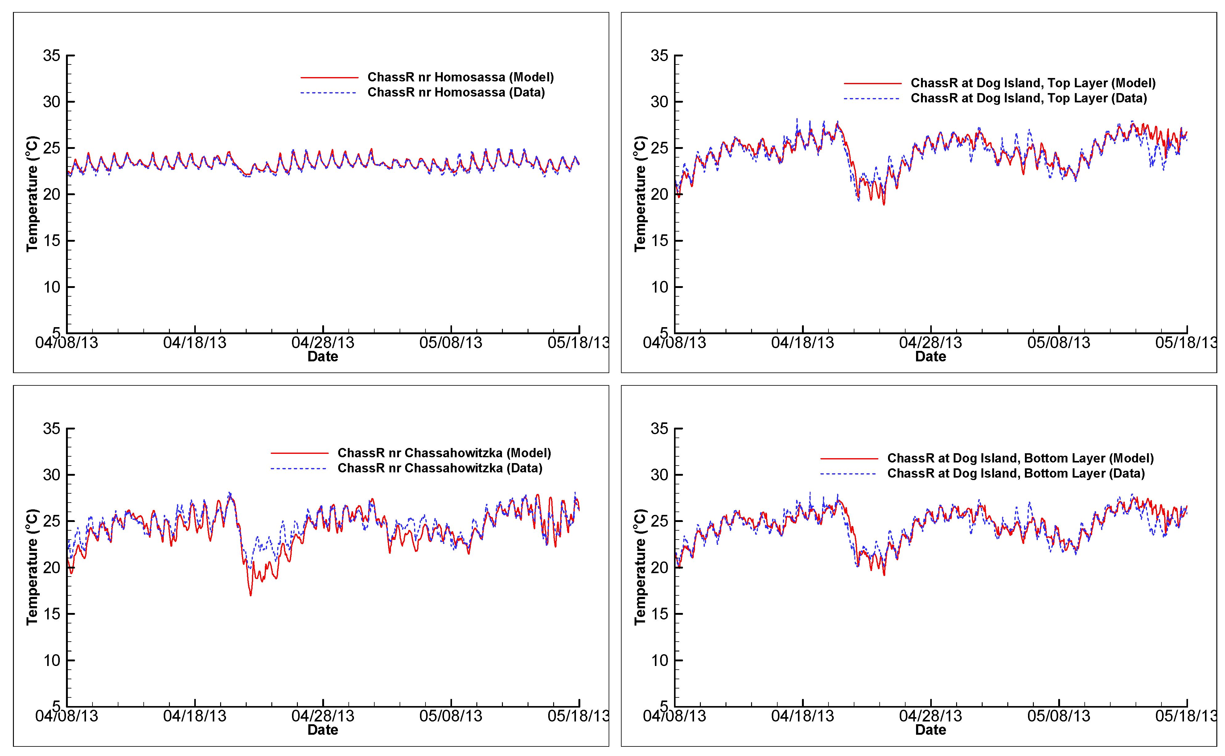
Table 4 shows that simulated temperatures have a mean error between −0.46 °C and 0.16 °C and a mean absolute error between 0.25 °C and 1.02 °C for the calibration period at the three USGS stations. During the verification period, the ME and MAE of simulated temperatures range between –0.36 °C and 0.16 °C and between 0.27 °C and 0.97 °C, respectively, while during the entire period, the ME and MAE ranges are from −0.43 °C to 0.16 °C and from 0.26 °C to 1.01 °C, respectively. RMSE and NRMSE between simulated and measured temperatures are respectively in the ranges of 0.32–1.38 °C and 0.032–0.068 for the calibration period, 0.35–1.26 °C and 0.025–0.060 for the verification period, and 0.33–1.36 °C and 0.027–0.063 for the entire period. R² values of simulated temperatures at the three USGS stations vary between 0.93 and 0.98, between 0.89 and 0.98, and between 0.91 and 0.98, respectively for the calibration, verification, and entire periods. Skills for simulated temperatures at the three stations range between 0.97 and 0.99 for the calibration period, between 0.957 and 0.995 for the verification period, and between 0.96 and 0.99 for the entire period. Overall, the ME, MAE, RMSE, NRMSE, R², and skill for simulated temperatures are −0.04 °C, 0.59 °C, 0.89 °C, and 0.031, 0.96, and 0.99, respectively among the three USGS stations.

Simulated discharge at the CRC station has a mean error of −0.002 m³/s, a mean absolute error of 0.02 m³/s, a root-mean-square error of 0.03 m³/s, a normalized RMSE of 0.037, an R² value of 0.96, and a skill of 0.99 during the calibration period. These statistics are 0.001 m³/s, 0.02 m³/s, 0.02 m³/s, 0.029, 0.97, and 0.99, respectively during the verification period. During the entire simulation period, the ME, MAE, RMSE, NRMSE, R², and the skill are −0.001 m³/s, 0.02 m³/s, 0.02 m³/s, 0.031, 0.96, and 0.99, respectively.

6. Conclusions

The laterally averaged hydrodynamic model LAMFE was applied to the Chassahowitzka River, a spring-fed estuary on the Gulf Coast of Florida, USA. The river is shallow and narrow, with a mean depth of 0.9 m and a width of 30 m or less in some upstream areas as well as its tributaries and distributaries. The downstream portion of the Chassahowitzka River has many braided channels, which are interconnected and flow through some coastal marsh complexes. The estuarine system is generally well or partially mixed and receives submarine groundwater discharges in the headspring area and in several tributaries.

In the model application, 348 longitudinal grids and 15 vertical layers were used to discretize the simulation domain of the Chassahowitzka River, with the grid length varying between 10 m to 370 m and the layer thickness varying between 0.3 m to 1.2 m. The model was calibrated and verified against measured real-time data of water level, salinity, and temperature in the Chassahowitzka River during a 52-month period between 18 November 2012 and 28 March 2017.

One of the difficulties in applying the LAMFE model to the Chassahowitzka River estuary is the need for the estimation of SGDs entering the tributaries, including the Crab, Potters, Baird, and Crawford Creeks. With the assumption that SGDs in the entire Chassahowitzka River system are driven by similar forces, SGDs entering these tributaries were estimated with a trial-and-error approach in the calibration process. Salinities and temperatures in the SGDs were also estimated using a trial-and-error approach.

Model calibration and verification are successfully conducted. Both visual comparisons and the statistical analyses of the differences between measured and simulated water levels, salinities, temperatures, and cross-sectional fluxes have shown that the LAMFE performs well in simulating hydrodynamics, salinity transport processes, and thermal dynamics in the Chassahowitzka River estuary. For example, Willmott skills for water elevation, salinity, and temperature simulations are 0.96, 0.91, and 0.98, respectively, while R² values for water elevation, salinity, and temperature simulations are 0.9, 0.74, and 0.96, respectively. Overall mean errors for water level, salinity, and temperature simulations are −3.20 cm, −0.08 psu, and −0.02 °C, respectively. Overall mean absolute errors for water level, salinity, and temperature simulations are 6.11 cm, 1.06 psu, and 0.57 °C, respectively.

For a relatively small area, tides at different locations are correlated, while the potentiometric surface is almost the same. Since the driving forces for the SGDs are mainly tides and the groundwater level, it can be assumed that SGDs out of all the spring vents in the Chassahowitzka River system are driven by the same or very similar forces. As a result, SGDs from different spring vents should be linearly correlated and have similar temporal variations, especially when a time scale of daily or longer is concerned. With this assumption, SGDs entering the Crab, Baird, Potters, and Crawford Creeks were estimated to be 53.0%, 5.8%, 22.4%, and 22.5%, respectively of that through the cross-section of the CRH station during the model calibration process. The good agreement of model results with field data suggests that the method used for the SGD estimation in the study is correct and offers a good reference for such an estimation in similar physical settings. Good comparisons of simulated and measured salinities and temperatures also suggest that estimates for salinity and temperature out of the spring vents are reasonable and can provide some useful information for other studies related to water quality and ecology of a spring system in the region.

As the submarine groundwater discharge to the Chassahowitzka River is a very important factor affecting the health of the estuary, it is recommended that more effort should be made in the future to measure rates of the SGD and other properties such as temperature and specific conductance for all of the identified spring vents. Although a perfect dataset of the SGD for the Chassahowitzka River is unfeasible due to some insurmountable difficulties in the data collection, new SGD measurements will certainly improve the SGD estimation and salinity and temperature estimations for the SGD and thus help future modeling efforts. A new bathymetry survey also needs to be conducted using the state-of-the-art technologies such as the integrated lidar-imagery sensor system CZMIL (Coastal Zone Mapping and Imaging Lidar) to obtain more details of the bathymetric variations in the river, so that an improved refinement of model grids in future simulations can be meaningfully done and some localized phenomenon can be accurately simulated.