
The Gradient-Boosting Method for Tackling High Computing Demand in Underwater Acoustic Propagation Modeling


Abstract
:1. Introduction
- to temporarily disable, for series of timesteps, the most costly modules (in terms of computing resources) of an ABM simulator;
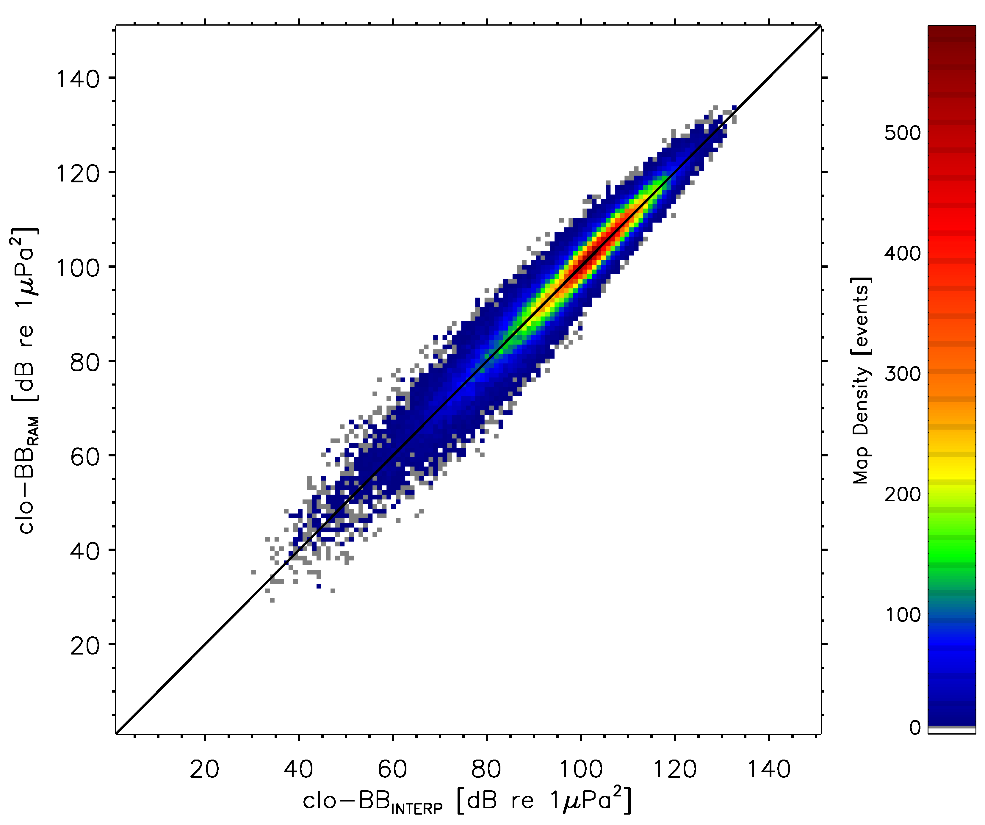
- to assess the performances of machine-learning methods to quickly interpolate, within reasonable uncertainties, missing values (that resulted from the said modules’ impairment) using fast-computed analytical approximations.
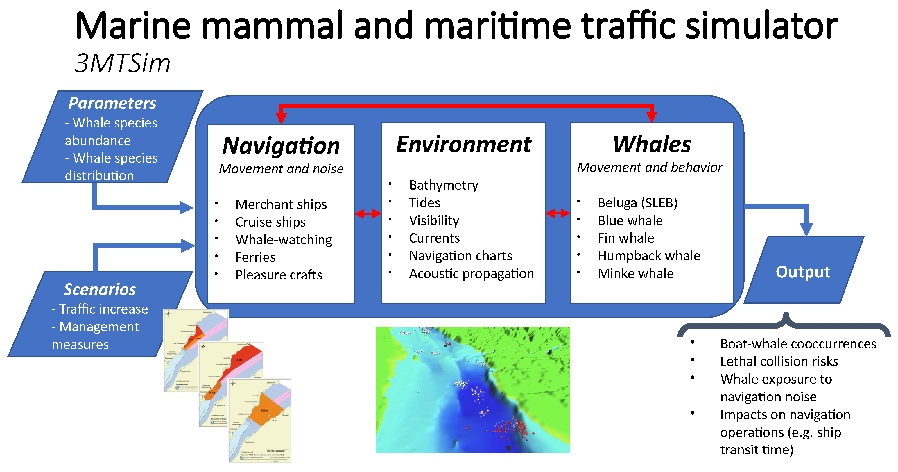
2. Marine Mammal and Maritime Traffic Simulator (3MTSim)
- Environment: this module was made of static (e.g., seabed composition) and dynamic processes (e.g., tides), which are known to influence whales, vessels and acoustic propagation.
- Vessels: the current version of the simulator included three broad categories of vessels, namely ocean-going commercial ships, cruise ships and whale-watching vessels. Ferry and pleasure craft submodules were in the development phase. Only ocean-going commercial ships and cruise ships were included in the current study and the simulated traffic was based on 2017 vessel movements obtained from AIS data (Table 1).
- Whales: five species were included in 3MTSim, namely beluga, blue, fin, humpback and minke whales. Only beluga whales were considered in this study and the datasets used to build the data-driven movement model are presented in Table 1.
- Acoustic: 3MTSim included a model of large ships’ monopole source levels (MSL) [20] and TL algorithms to cover the broad range of frequencies relevant to the beluga, i.e., see Collins [1]’s RAM for f ≲ 1000 Hz and Porter and Liu [2]’s Bellhop for f ≳ 1000 Hz. The current study focused on low frequencies as they allow for isolating changes in RL with shipping—the focal traffic component in the study—from those of smaller watercraft. Moreover, high absorption and instrumentation challenges have led to very limited development of medium to high frequency models of ships’ MSL [22].
3. The Gradient-Boosting Method (GBM)
4. Acoustic Methods
5. Data Processing
- the clo-BB prediction, available at each timestep for each ship-to-animal encounter;
- a crude approximation of the clo-BB prediction, referred to as BB, and provided by the linear interpolation of the two closest, non-missing clo-BB values preserved, i.e., those with timestep numbers that were divisible by 10 (e.g., 1400, 1410, 1420, …, 2880, 2890, 2900, …, 5020, 5030, 5040);
- a 20-element 1-D vector representing the bathymetric profile along the line of sight connecting the ship and the animal. Giving that our bathymetric data had a resolution of 100 m pixel (see Table 1), any separation above 2000 m between a ship and a beluga implied a spatial degradation of the bathymetric information used by 3MTSim. We therefore expected that the uncertainty on the GBM output should increase with increasing ship-to-animal separation.
6. Validation
7. Conclusions
Author Contributions
Funding
Institutional Review Board Statement
Informed Consent Statement
Data Availability Statement
Acknowledgments
Conflicts of Interest
Abbreviations
| 3MTSim | Marine Mammal and Maritime Traffic Simulator; |
| ABM | agent-b model; |
| AIS | automatic identification system; |
| BB | broadband; |
| EST | Eastern Standard Time; |
| GBM | gradient-boosting method; |
| GREMM | Groupe de Recherche et d’Éducation sur les Mammifères Marins; |
| GT | ground truth; |
| HRA | high-residency area; |
| MSLs | monopole source levels; |
| OGSL | Observatoire Global du Saint-Laurent; |
| RL | received levels; |
| SIM | Système d’Information Maritime; |
| SLE | St. Lawrence Estuary; |
| TL | transmission loss; |
| VHF | very-high frequency; |
| XGBoost | eXtreme Gradient Boosting algorithm. |
Appendix A
- At a given timestep, 3MTSim established if a direct line of sight existed between a ship and an animal (see Section 2 for the definition for line of sight).
- If so, for each central frequency in Table 2’s middle column, the ship’s MSLs were calculated using its static and dynamic properties as described by Wittekind [20].
- (a)
- These properties were as follows:
- i
- The cavitation inception speed (), which was fixed at 10 knots;
- ii
- The block coefficient (), which is the ratio of the ship’s underwater volume to the volume of a rectangular block having the same overall length (ℓ), breadth (b) and depth/draught (d); calculation of the block coefficient as a function of the ship’s length (ℓ) and speed through water (v) was provided by (Barrass [28] Chapter 1);
- iii
- The ship’s displacement () in tons was provided by the mass of water contained in a × ℓ × b × d volume;
- iv
- A single (n = 1) resiliently mounted (E = 0) engine of mass m = 200 tons was arbitrarily attributed to all ships.
- (b)
- MSLs were assumed to be constant inside a given 1/3-octave band and, therefore, were split and equally re-distributed for each integer frequency in that said band (i.e., in order that the integration across the band’s lower and upper limits gave the initial 1/3-octave MSL prediction; see Table 2).
The result for Step 2 was a 1112-element 1-D vector, in units of dB Hz re 1 Pa, providing the ship’s MSLs for each integer frequency between 11 and 1122 Hz. - TL along the line of sight connecting the ship to the animal was computed for each central frequency in Table 2’s middle column. This was performed twice using the following two distinct models.
- (a)
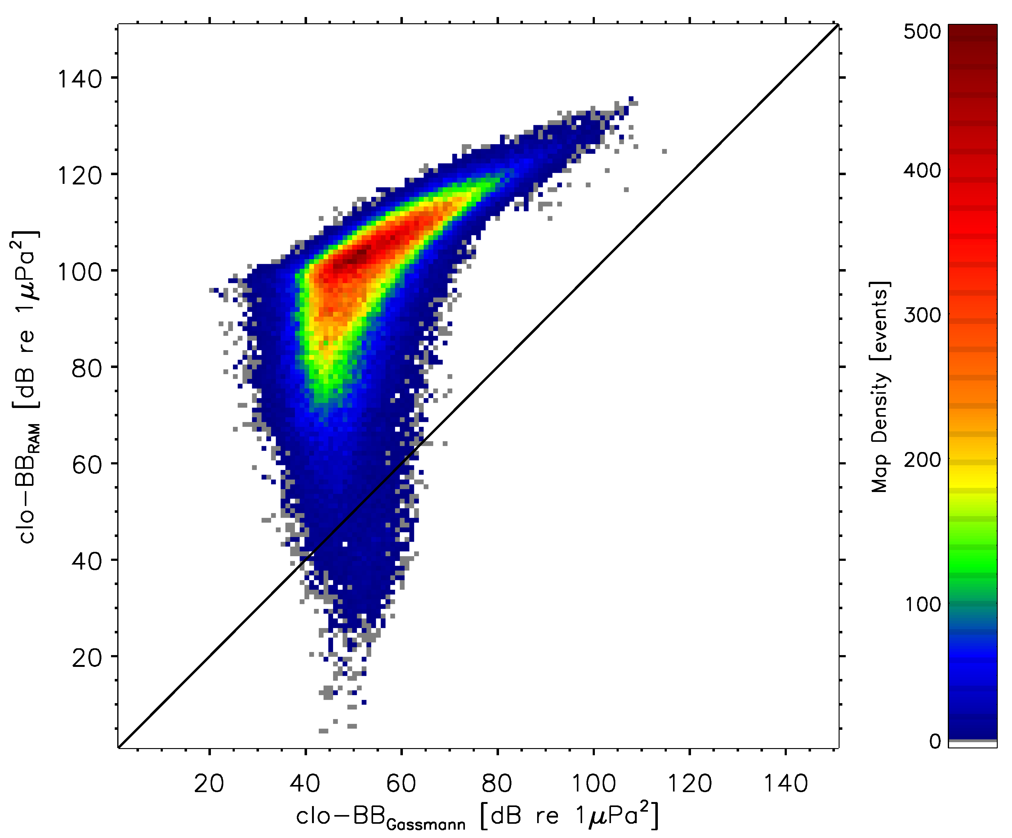
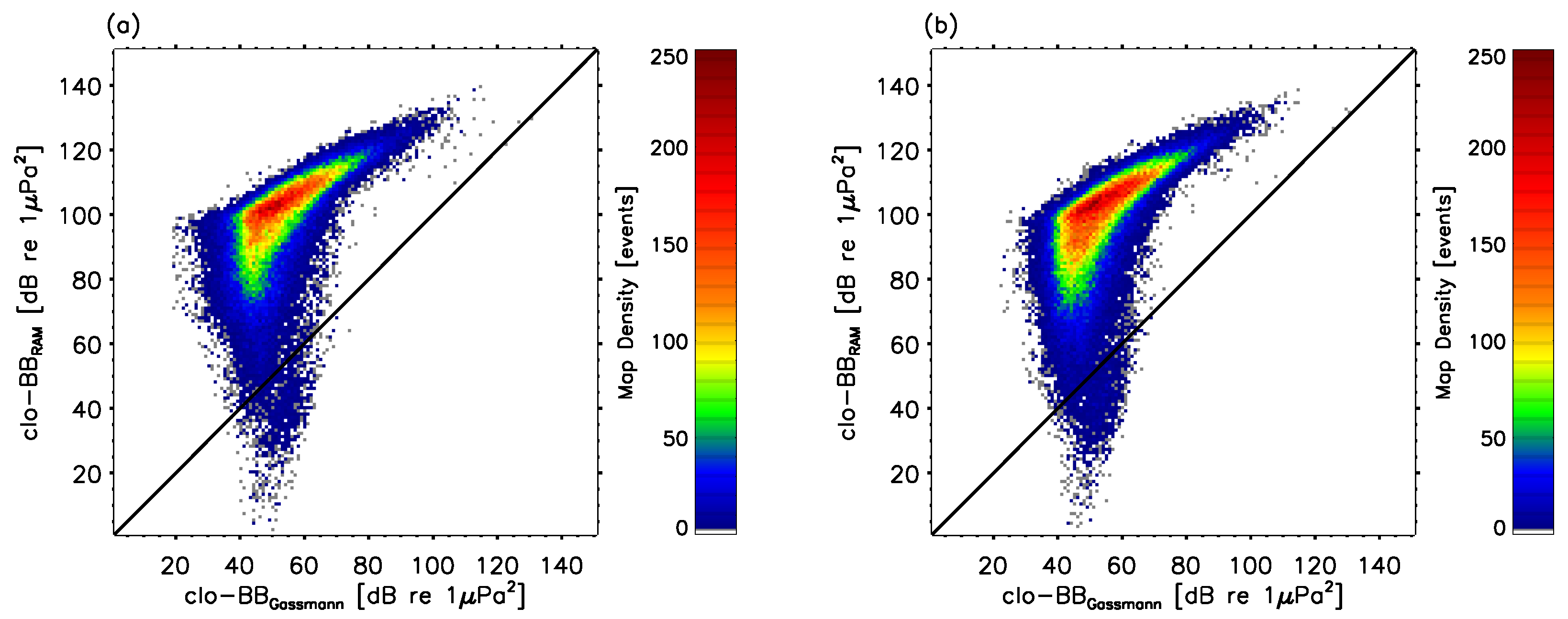
- The split-step Padé approximation of the parabolic equation method [1]. The RAM model was time-consuming but was numerically reliable and highly range-dependent. Properties in bathymetry, sediments type and sound speed gradients were implemented in the 3MTSim platform (see Table 1). The RAM model provided TL in units of dB Hz re 1 Pa.
- (b)
- The analytical solution provided by Gassmann et al. [26] was given as:where r is the distance, in meters, separating the source from the receiver, f is the sound frequency in Hertz, is the source depth (i.e., 70% of the ship’s draught d according to ISO 17208-2 [29]) in meters, is the receiver’s depth in meters and is the water’s mean sound speed, in m s along the transect connecting the source and the receiver.Totally negligible in terms of computing time, Equation (A1) (hereafter referred as the Gassmann model) corrected for sound attenuation attributed to surface reflections (i.e., Lloyd’s mirror effects) but is range-independent and does not consider variations of the geomorphological terrain and physico-chemical properties along lines of sight connecting sources and receivers. The Gassmann model also provided TL in units of dB Hz re 1 Pa.
TL was assumed to be constant inside a given 1/3-octave band and, therefore, predictions were assumed equal for each integer frequency in that said band. The results for Step 3 were two 1112-element 1-D vectors, in units of dB Hz re 1 Pa, providing TL across the ship-to-animal transect for each integer frequency between 11 and 1122 Hz, one 1112-element 1-D vector for each of the two TL models discussed above. - Noise levels radiated at the source and received at the animal’s position were linked by the passive SONAR equation:where (,) and (,) are respectively the ship’s and animal’s positions and TL(,→,) is the TL sustained by the sound wave from (,) to (,).From Equation (A2), subtraction of a TL vector (see Step 3) from the MSL vector (see Step 2) yielded a 1112-element 1-D vector, in units of dB Hz re 1 Pa, of the instantaneous sound pressure RL at the position of the animal for each integer frequency between 11 and 1122 Hz, as predicted by the TL model used. For the purpose of this work and sake of simplicity, sound absorption attributed to magnesium sulfate and boric acid in seawater (see François and Garrison [30,31]) was ignored in the computation of RL.
- The RL calculation (see Step 4) was repeated for all k ships with direct lines of sight with the animal during the said timestep. The individual 1112-element RL contributions were then summed, frequency-by-frequency, as non-coherent sources according to the following equation:Once Equation (A3) was carried out on all integer frequencies between 11 and 1122 Hz, RL corresponded to a 1112-element 1-D vector, in units of dB Hz re 1 Pa, of the instantaneous sound pressure RL predicted at the position of the animal and attributed to all k ships with direct lines of sight at this timestep.
- Integration over the frequency domain of the RL vector (see Step 5) provided the BB measurement, in units of dB re 1 Pa, between 11 and 1122 Hz of all noise contributors with direct lines of sight to the position of the animal:At each timestep, for each animal exposed to at least one ship, two BB predictions were computed; one obtained from the RAM TL model and the other from the analytic TL approximation of Gassmann et al. [26] (see Step 3).

| (a) Whales’ Output .txt File. |
| Beluga ID number |
| Random seed |
| Timestep |
| X of the whale |
| Y of the whale |
| Depth of the whale |
| BB received by the whale |
| BB received by the whale |
| TL.b01 from the closest ship only |
| ⋯ to ⋯ |
| TL.b20 from the closest ship only |
| TL.b01 from the closest ship only |
| ⋯ to ⋯ |
| TL.b20 from the closest ship only |
| (b) Ships’ Output .txt File. |
| Beluga ID number |
| Random seed |
| Timestep |
| Number of ships with direct line-of-sight |
| X of the closest ship |
| Y of the closest ship |
| Distance to the closest ship |
| Length of the closest ship |
| Width of the closest ship |
| Draught of the closest ship |
| Speed through water of the closest ship |
| X of the second closest ship |
| ⋯ to ⋯ |
| Speed through water of the second closest ship |
| X of the third closest ship |
| ⋯ to ⋯ |
| Speed through water of the third closest ship |
| X of the fourth closest ship |
| ⋯ to ⋯ |
| Speed through water of the fourth closest ship |
| X of the fifth closest ship |
| ⋯ to ⋯ |
| Speed through water of the fifth closest ship |
Appendix B
| Tick | ID | e-UTM | n-UTM | Depth | e-UTM | n-UTM | Speed | Distance | clo-BB | clo-BB |
|---|---|---|---|---|---|---|---|---|---|---|
| (m) | (m) | (m) | (m) | (m) | (knots) | (m) | (dB re 1 Pa) | (dB re 1 Pa) | ||
| 7220 | 77 | 497,624 | 5,361,030 | 1.0 | 493,200 | 5,360,600 | 16.11 | 4100 | 107.97 | 63.98 |
| 7221 | 77 | 497,947 | 5,360,968 | 1.0 | 494,100 | 5,361,300 | 16.19 | 3700 | 108.33 | 65.78 |
| 7222 | 77 | 497,991 | 5,360,993 | 1.0 | 495,000 | 5,361,900 | 15.94 | 3100 | 113.82 | 68.78 |
| 7223 | 77 | 498,524 | 5,361,345 | 1.0 | 495,900 | 5,362,500 | 16.38 | 2800 | 111.52 | 70.68 |
| 7224 | 77 | 498,815 | 5,361,989 | 1.0 | 496,800 | 5,363,100 | 16.04 | 2400 | 113.56 | 73.26 |
| 7225 | 77 | 499,011 | 5,362,451 | 1.0 | 497,700 | 5,363,700 | 16.10 | 2000 | 116.01 | 76.44 |
| 7226 | 77 | 499,536 | 5,363,255 | 1.0 | 498,500 | 5,364,400 | 16.17 | 1800 | 117.80 | 78.29 |
| 7227 | 77 | 499,656 | 5,364,058 | 1.0 | 499,400 | 5,365,000 | 16.02 | 1500 | 119.46 | 81.41 |
| 7228 | 77 | 500,132 | 5,364,392 | 1.0 | 500,300 | 5,365,600 | 16.10 | 1500 | 119.44 | 81.44 |
| 7229 | 77 | 500,754 | 5,364,353 | 1.0 | 501,200 | 5,366,200 | 16.30 | 2100 | 115.69 | 75.65 |
| 7230 | 77 | 501,482 | 5,364,384 | 1.0 | 502,100 | 5,366,800 | 16.08 | 2700 | 112.26 | 71.22 |
| 7231 | 77 | 501,904 | 5,364,473 | 1.0 | 503,000 | 5,367,400 | 16.09 | 3400 | 115.15 | 67.22 |
| 7232 | 77 | 503,203 | 5,364,544 | 1.0 | 503,900 | 5,368,000 | 16.09 | 3700 | 107.98 | 65.75 |
| 7233 | 77 | 503,548 | 5,364,437 | 1.0 | 504,800 | 5,368,600 | 16.19 | 4400 | 107.87 | 62.77 |
| 7234 | 77 | 504,280 | 5,364,252 | 1.0 | 505,700 | 5,369,200 | 16.21 | 5200 | 101.09 | 59.88 |
| 7235 | 77 | 504,656 | 5,364,348 | 1.0 | 506,600 | 5,369,800 | 16.26 | 5900 | 102.12 | 57.70 |
| 7236 | 77 | 505,210 | 5,364,303 | 1.0 | 507,500 | 5,370,400 | 16.25 | 6700 | 97.75 | 55.48 |
| 7237 | 77 | 505,798 | 5,364,046 | 4.0 | 508,500 | 5,371,000 | 16.95 | 7400 | 92.65 | 53.94 |
| 7238 | 77 | 505,024 | 5,363,184 | 8.0 | 509,400 | 5,371,600 | 16.16 | 8800 | 98.21 | 66.28 |
| 7239 | 77 | 504,457 | 5,362,150 | 8.0 | 510,300 | 5,372,200 | 15.38 | 11,400 | 96.14 | 64.05 |
| 7240 | 77 | 503,876 | 5,361,745 | 4.0 | 511,200 | 5,372,800 | 15.34 | 13,100 | 90.82 | 59.12 |
| Tick | ID | clo-BB | BB | ⋯ | clo-BB | Deviation | ||
|---|---|---|---|---|---|---|---|---|
| (dB re 1 Pa) | (dB re 1 Pa) | (m) | (m) | (m) | (dB re 1 Pa) | (dB re 1 Pa) | ||
| 7220 | 77 | 63.98 | 107.97 | 236 | ⋯ | 166 | 107.97 | 0.00 |
| 7221 | 77 | 65.78 | 108.40 | 237 | ⋯ | 160 | 111.20 | 2.87 |
| 7222 | 77 | 68.78 | 108.83 | 239 | ⋯ | 160 | 113.28 | 0.54 |
| 7223 | 77 | 70.68 | 109.26 | 237 | ⋯ | 157 | 114.47 | 2.95 |
| 7224 | 77 | 73.26 | 109.69 | 230 | ⋯ | 164 | 114.93 | 1.37 |
| 7225 | 77 | 76.44 | 110.12 | 224 | ⋯ | 172 | 116.87 | 0.86 |
| 7226 | 77 | 78.29 | 110.54 | 229 | ⋯ | 180 | 117.44 | 0.36 |
| 7227 | 77 | 81.41 | 110.97 | 229 | ⋯ | 200 | 118.06 | 1.40 |
| 7228 | 77 | 81.44 | 111.40 | 228 | ⋯ | 200 | 118.85 | 0.59 |
| 7229 | 77 | 75.65 | 111.83 | 228 | ⋯ | 118 | 117.14 | 1.45 |
| 7230 | 77 | 71.22 | 112.26 | 227 | ⋯ | 167 | 112.26 | 0.00 |
| 7231 | 77 | 67.22 | 110.12 | 225 | ⋯ | 137 | 112.68 | 2.47 |
| 7232 | 77 | 65.75 | 107.97 | 221 | ⋯ | 92 | 109.75 | 1.77 |
| 7233 | 77 | 62.77 | 105.83 | 207 | ⋯ | 80 | 108.13 | 0.26 |
| 7234 | 77 | 59.88 | 103.68 | 197 | ⋯ | 73 | 103.64 | 2.55 |
| 7235 | 77 | 57.70 | 101.54 | 196 | ⋯ | 67 | 101.46 | 0.66 |
| 7236 | 77 | 55.48 | 99.40 | 198 | ⋯ | 54 | 99.47 | 1.72 |
| 7237 | 77 | 53.94 | 97.25 | 200 | ⋯ | 47 | 94.28 | 1.63 |
| 7238 | 77 | 66.28 | 95.11 | 200 | ⋯ | 44 | 102.78 | 4.57 |
| 7239 | 77 | 64.05 | 92.96 | 188 | ⋯ | 38 | 98.92 | 2.78 |
| 7240 | 77 | 59.12 | 90.82 | 196 | ⋯ | 35 | 90.82 | 0.00 |
References
- Collins, M.D. A Split-Step Padé Solution for the Parabolic Equation Method. J. Acoust. Soc. Am. 1993, 93, 1736–1742. [Google Scholar] [CrossRef]
- Porter, M.B.; Liu, Y.C. Finite-Element Ray Tracing. Theor. Comput. Acoust. 1994, 2, 947–956. [Google Scholar]
- Mortensen, L.O.; Chudzinska, M.E.; Slabbekoorn, H.; Thomsen, F. Agent-based models to investigate sound impact on marine animals: Bridging the gap between effects on individual behaviour and population level consequences. Oikos 2021, 130, 1074–1086. [Google Scholar] [CrossRef]
- Helbing, D. Agent-based modeling. In Social Self-Organization; Springer: Berlin/Heidelberg, Germany, 2012; pp. 25–70. [Google Scholar]
- Castle, C.J.E.; Crooks, A.T. Principles and Concepts of Agent-Based Modelling for Developing Geospatial Simulations; Technical Report; University College London: London, UK, 2006. [Google Scholar]
- Couclelis, H. Modeling frameworks, paradigms, and approaches. In Geographic Information Systems and Environmental Modeling; Prentice Hall: Hoboken, NJ, USA, 2002; pp. 36–50. [Google Scholar]
- Axtell, R. Why agents?: On the varied motivations for agent computing in the social sciences. In Center on Social and Economic Dynamics; Academia: Cambridge, MA, USA, 2000; pp. 1–24. [Google Scholar]
- Chion, C.; Bonnell, T.R.; Lagrois, D.; Michaud, R.; Lesage, V.; Dupuch, A.; McQuinn, I.H.; Turgeon, S. Agent-based modelling reveals a disproportionate exposure of females and calves to a local increase in shipping and associated noise in an endangered beluga population. Mar. Pollut. Bull. 2021, 173, 112977. [Google Scholar] [CrossRef]
- Trigg, L.E.; Chen, F.; Shapiro, G.I.; Ingram, S.N.; Embling, C.B. An adaptive grid to improve the efficiency and accuracy of modelling underwater noise from shipping. Mar. Pollut. Bull. 2018, 131, 589–601. [Google Scholar] [CrossRef] [PubMed] [Green Version]
- Chion, C.; Lagrois, D.; Dupras, J.; Turgeon, S.; McQuinn, I.H.; Michaud, R.; Ménard, N.; Parrott, L. Underwater Acoustic Impacts of Shipping Management Measures: Results from a Social-Ecological Model of Boat and Whale Movements in the St. Lawrence River Estuary (Canada). Ecol. Model. 2017, 354, 72–87. [Google Scholar] [CrossRef]
- Parrott, L.; Chion, C.; Martins, C.C.A.; Lamontagne, P.; Turgeon, S.; Landry, J.A.; Zhens, B.; Marceau, D.J.; Michaud, R.; Cantin, G.; et al. A Decision Support System to Assist the Sustainable Management of Navigation Activities in the St. Lawrence River Estuary, Canada. Environ. Model. Softw. 2011, 26, 1403–1418. [Google Scholar] [CrossRef]
- Aulanier, F.; Simard, Y.; Roy, N.; Gervaise, C.; Bandet, M. Spatial-Temporal Exposure of Blue Whale Habitats to Shipping Noise in St. Lawrence System; Fisheries and Oceans Canada, Ecosystems and Oceans Science: Ottawa, ON, Canada, 2016.
- Aulanier, F.; Simard, Y.; Roy, N.; Bandet, M.; Gervaise, C. Groundtruthed Probabilistic Shipping Noise Modeling and Mapping: Application to Blue Whale Habitat in the Gulf of St. Lawrence. Proc. Meet. Acoust. 2016, 27, 070006. [Google Scholar]
- Chion, C.; Parrott, L.; Landry, J.A. Collisions et Cooccurrences entre Navires Marchands et Baleines dans l’Estuaire du Saint-Laurent; Technical Report; Fisheries and Oceans Canada: Ottawa, ON, Canada, 2012.
- Chion, C.; Cantin, G.; Dionne, S.; Dubeau, B.; Lamontagne, P.; Landry, J.A.; Marceau, D.; Martins, C.C.A.; Ménard, N.; Michaud, R.; et al. Spatiotemporal Modelling for Policy Analysis: Application to Sustainable Management of Whale-Watching Activities. Mar. Policy 2013, 38, 151–162. [Google Scholar] [CrossRef]
- Chion, C. An Agent-Based Model for the Sustainable Management of Navigation Activities in the Saint-Lawrence Estuary. Ph.D. Thesis, École de Technologie Supérieure, Montréal, QC, Canada, 2011. [Google Scholar]
- Chion, C.; Lamontagne, P.; Turgeon, S.; Parrott, L.; Landry, J.A.; Marceau, D.J.; Martins, C.C.A.; Michaud, R.; Ménard, N.; Cantin, G.; et al. Eliciting Cognitive Processes Underlying Patterns of Human-Wildlife Interactions for Agent-Based Modelling. Ecol. Model. 2011, 222, 2213–2226. [Google Scholar] [CrossRef]
- Jensen, F.B.; Kuperman, W.A.; Porter, M.B.; Schmidt, H. Computational Ocean Acoustics; Springer Science & Business Media: New York, NY, USA, 2011. [Google Scholar]
- Loring, D.H.; Nota, D.J.G. Morphology and Sediments of the Gulf of St. Lawrence; Fisheries and Marine Service: Ottawa, ON, Canada, 1973.
- Wittekind, D.K. A Simple Model for the Underwater Noise Source Level of Ships. J. Ship Prod. Des. 2014, 30, 7–14. [Google Scholar] [CrossRef]
- McQuinn, I.H.; Lesage, V.; Carrier, D.; Larrivée, G.; Samson, Y.; Chartrand, S.; Michaud, R.; Theriault, J. A Threatened Beluga (Delphinapterus Leucas) Population in the Traffic Lane: Vessel-Generated Noise Characteristics of the Saguenay–St. Lawrence Marine Park, Canada. J. Acoust. Soc. Am. 2011, 130, 3661–3673. [Google Scholar] [CrossRef] [PubMed]
- Hermannsen, L.; Beedholm, K.; Tougaard, J.; Madsen, P.T. High Frequency Components of Ship Noise in Shallow Water with a Discussion of Implications for Harbor Porpoises (Phocoena Phocoena). J. Acoust. Soc. Am. 2014, 136, 1640–1653. [Google Scholar] [CrossRef] [PubMed] [Green Version]
- Awbrey, F.T.; Thomas, J.A.; Kastelein, R.A. Low-frequency underwater hearing sensitivity in belugas, Delphinapterus leucas. J. Acoust. Soc. Am. 1988, 84, 2273–2275. [Google Scholar] [CrossRef]
- Friedman, J.H. Greedy Function Approximation: A Gradient Boosting Machine. Ann. Stat. 2001, 29, 1189–1232. [Google Scholar] [CrossRef]
- Chen, T.; Guestrin, C. Xgboost: A scalable tree boosting system. In Proceedings of the 22nd ACM Sigkdd International Conference on Knowledge Discovery and Data Mining, San Francisco, CA, USA, 13–17 August 2016; pp. 785–794. [Google Scholar]
- Gassmann, M.; Wiggins, S.M.; Hildebrand, J.A. Deep-Water Measurements of Container Ship Radiated Noise Signatures and Directionality. J. Acoust. Soc. Am. 2017, 142, 1563–1574. [Google Scholar] [CrossRef] [PubMed] [Green Version]
- Sponagle, N. Variability of Ship Noise Measurements; Technical Report; Defense Research Establishment Atlantic: Halifax, NS, Canada, 1988. [Google Scholar]
- Barrass, B. Ship Design and Performance for Masters and Mates; Elsevier: Oxford, UK, 2004. [Google Scholar]
- ISO 17208-2; Underwater Acoustics—Quantities and Procedures for Description and Measurements of Underwater Sound from Ships—Part 2: Determination of Source Levels from Deep Water Measurements. Technical Report; International Standardization Organization: Geneva, Switzerland, 2019.
- François, R.E.; Garrison, G.R. Sound absorption based on ocean measurements: Part I: Pure water and magnesium sulfate contributions. J. Acoust. Soc. Am. 1982, 72, 896–907. [Google Scholar] [CrossRef]
- François, R.E.; Garrison, G.R. Sound absorption based on ocean measurements. Part II: Boric acid contribution and equation for total absorption. J. Acoust. Soc. Am. 1982, 72, 1879–1890. [Google Scholar] [CrossRef]

| Dataset | Reference | Time Frame | Description | Module |
|---|---|---|---|---|
| Beluga photo ID | GREMM | 1989–2007 (June–October) | Community and spatial structure | Beluga population |
| Beluga photo ID | GREMM | 1989–2007 (June–October) | Community and spatial structure | Beluga population |
| Beluga VHF telemetry tracking and diving patterns | Fisheries and Oceans Canada and GREMM | 2001–2005 | 3D-movement patterns | Beluga population |
| Tracking of beluga herds | GREMM | 1989–2017 (June–October) | Communities’ territorial appropriation | Beluga population |
| Beluga spatial distribution from aerial surveys | Fisheries and Oceans Canada | 1990–2009 (August) | Population summer spatial distribution and high-density areas | Beluga population |
| AIS data | Canadian Coast Guard | 2011–2018 | Description of the marine traffic in the beluga habitat | Navigation |
| SIM data | Innovation Maritime | 2018–2019 | Quantitative information on the merchant fleet | Navigation |
| Bathymetry | Canadian Hydrographic Service | N.A. | 2D chart providing depth values across the simulator’s computational area (resolution = 100 m) | Navigation & Acoustic |
| Seabed geoacoustic properties | [18,19] | N.A. | Geoacoustic properties retrieved from the sediments’ nature | Acoustic |
| Water column geoacoustic properties | OGSL | 2004–2018 (summer) | (1) Temperature and salinity profiles as a function of depth in areas of interest (resolution = 1 m) | Acoustic |
| (2) Conversion in speed-of-sound profiles as a function of depth | ||||
| (3) Polynomial fitting of the speed-of-sound profiles | ||||
| MSL signatures of merchant ships | [20] | N.A. | Frequency-dependent model providing the amplitude of the sound emitted by a source as a function of the source’s static (e.g., length, width, draught) and dynamic (speed) properties | Acoustic |
| Noise levels in the summer habitat of the beluga | [21] | 2004–2005 | Noise levels measured at a depth of 15 m in different areas of interest | Acoustic |
| Band Name | Lower Band Limit | Central Frequency | Upper Band Limit |
|---|---|---|---|
| (Hz) | (Hz) | (Hz) | |
| b01 | 11 | 12 | 13 |
| b02 | 14 | 16 | 17 |
| b03 | 18 | 20 | 21 |
| b04 | 22 | 25 | 27 |
| b05 | 28 | 32 | 35 |
| b06 | 36 | 40 | 44 |
| b07 | 45 | 50 | 55 |
| b08 | 56 | 63 | 70 |
| b09 | 71 | 80 | 88 |
| b10 | 89 | 100 | 111 |
| b11 | 112 | 125 | 140 |
| b12 | 141 | 160 | 177 |
| b13 | 178 | 200 | 223 |
| b14 | 224 | 250 | 281 |
| b15 | 282 | 315 | 354 |
| b16 | 355 | 400 | 446 |
| b17 | 447 | 500 | 561 |
| b18 | 562 | 630 | 707 |
| b19 | 708 | 800 | 890 |
| b20 | 891 | 1000 | 1122 |
| Seed | Start Date | Local Time | Computing Time | Pairs | Average Deviation |
|---|---|---|---|---|---|
| (hours) | (dB re 1 Pa) | ||||
| GT | 4 Feb 2021 | 17:55 | 39.37 | 214,438 | 3.23 ± 3.76(1) |
| 20 | 9 Feb 2021 | 03:40 | 36.75 | 173,492 | 3.11 ± 3.72(1) |
| 30 | 10 Feb 2021 | 17:05 | 36.25 | 172,175 | 3.24 ± 3.89(1) |
| 40 | 12 Feb 2021 | 12:30 | 40.08 | 201,356 | 3.24 ± 3.84(1) |
| 50 | 14 Feb 2021 | 12:40 | 41.02 | 198,940 | 3.13 ± 3.71(1) |
| 60 | 16 Feb 2021 | 13:05 | 34.90 | 164,220 | 3.12 ± 3.76(1) |
Publisher’s Note: MDPI stays neutral with regard to jurisdictional claims in published maps and institutional affiliations. |
© 2022 by the authors. Licensee MDPI, Basel, Switzerland. This article is an open access article distributed under the terms and conditions of the Creative Commons Attribution (CC BY) license (https://creativecommons.org/licenses/by/4.0/).
Share and Cite
Lagrois, D.; Bonnell, T.R.; Shukla, A.; Chion, C. The Gradient-Boosting Method for Tackling High Computing Demand in Underwater Acoustic Propagation Modeling. J. Mar. Sci. Eng. 2022, 10, 899. https://doi.org/10.3390/jmse10070899
Lagrois D, Bonnell TR, Shukla A, Chion C. The Gradient-Boosting Method for Tackling High Computing Demand in Underwater Acoustic Propagation Modeling. Journal of Marine Science and Engineering. 2022; 10(7):899. https://doi.org/10.3390/jmse10070899
Chicago/Turabian StyleLagrois, Dominic, Tyler R. Bonnell, Ankita Shukla, and Clément Chion. 2022. "The Gradient-Boosting Method for Tackling High Computing Demand in Underwater Acoustic Propagation Modeling" Journal of Marine Science and Engineering 10, no. 7: 899. https://doi.org/10.3390/jmse10070899
APA StyleLagrois, D., Bonnell, T. R., Shukla, A., & Chion, C. (2022). The Gradient-Boosting Method for Tackling High Computing Demand in Underwater Acoustic Propagation Modeling. Journal of Marine Science and Engineering, 10(7), 899. https://doi.org/10.3390/jmse10070899