Numerical Study of Topographic Effects on Wind-Driven Coastal Upwelling on the Scotian Shelf

Abstract

Wind-driven coastal upwelling can cause a sudden drop in sea surface temperatures (SSTs) of up to more than 8 °C on the inner Scotian Shelf (ScS) in the summer months. Three major coastal upwelling events on the ScS in the summer of 2012 are analyzed using in-situ SST observations and satellite remote sensing SST data. A spatial correlation analysis of satellite SST data shows an asymmetric distribution in the along-shore direction with smaller correlation coefficients in the downstream area than in the upstream area over the inner ScS during upwelling events. A regression analysis indicates that the wind impulse plays a major role in generating the SST cooling during the initial response stage of upwelling events. A nested-grid ocean circulation model (DalCoast-CSS) is used to examine the effect of irregular coastline and rugged bathymetry on the spatial and temporal variability of wind-driven upwelling over the inner ScS. The model has four submodels downscaling from the eastern Canadian Shelf to the central ScS. The model external forcing includes tides, winds, river discharges, and net heat flux at the sea surface. A comparison of model results with the satellite SST data reveals a satisfactory performance of the model in reproducing the development of coastal upwelling on the ScS. Model results demonstrate that the irregular coastline and rugged bathymetry play important roles in influencing the temporal and spatial evolution of the upwelling plume over the inner ScS. The irregular coastline (e.g., cape) is responsible for the relatively warm SSTs in two downstream inlets (i.e., St. Margarets Bay and Mahone Bay) and adjacent coastal waters. The rugged bathymetry (e.g., submerged bank) influences the spatial extent of filaments through the advection process.

1. Introduction

Coastal upwelling is an important oceanographic process that sustains many productive fisheries and marine ecosystems around the globe [1]. It is a prominent year-long phenomenon at tropical-subtropical latitudes near the eastern boundaries of both the Atlantic and Pacific basins. It is also one of the well-recognized seasonal phenomena in many other locations (e.g., Somalia, Yemen, Oman, southwest India, southern Australia, southeastern China, and the east and west coasts of Canada [1,2,3,4]).

Coastal upwelling occurs on the Scotian Shelf, eastern Canada (ScS, Figure 1) when the region is experiencing southwesterly winds blowing parallel to the south shore of Nova Scotia. The surface water flows offshore, according to the classic Ekman theory developed in 1905 [5], and is replaced by cool and nutrient-rich water, which rises up into the coastal area from below, resulting in the wind-driven upwelling phenomena.

Coastal upwelling on the ScS has been the subject of several studies in the past. The first report of coastal upwelling on the ScS was made by Hachey in 1937 [6], and showed that strong southwesterly winds are highly correlated with lower-than-normal sea surface temperature (SST) conditions off the coast of Nova Scotia. Satellite images of SST demonstrated the development of a band of cool surface waters over the inner ScS during a month-long period of upwelling-favorable winds in the summer of 1984 [4]. Donohue, in 2001 [7], simulated the upwelling event in 1984 by using the Princeton Ocean Model (POM) forced by idealized spatially uniform winds and suggested that realistic bathymetry is required to reproduce the observed cold water band along the coast. More recently, Laurent, in 2011 [8], examined the biological response to the upwelling in Lunenburg Bay, which is a coastal embayment on the coast of Nova Scotia. Laurent found that the observed chlorophyll concentration in the Bay was 1.1 ± 0.6 mg m⁻³ during mixed upwelling and downwelling events in summer, which is small compared to the typical value (>5 mg m⁻³) in the well-studied eastern boundary upwelling systems. Laurent attributed this limited response of phytoplankton variability in the Bay to the rapid wind-driven flushing and the low nitrate concentration in the ScS water.

The above and other studies suggested that both winds and bathymetry play crucial roles on the coastal upwelling on the ScS. Several important questions remain to be investigated, such as what is the temporal and spatial variability of coastal upwelling over the inner ScS under realistic wind forcing, and what is the major effect of bathymetric irregularities on the wind-driven coastal upwelling over the study region. In this study, we address these questions based on the observations made by various instruments and numerical results produced by a nested-grid circulation model (DalCoast-CSS). A process study is conducted by using DalCoast-CSS to examine the role of irregular coastline and rugged bathymetry on the evolution of the coastal upwelling plume.

This paper is structured as follows. In Section 2, the observations and the nested-grid circulation modelling system used in this study are described. In Section 3, the observed upwelling on the ScS is analyzed. In Section 4, the model results during upwelling events are compared with observations. A process study is conducted to investigate the role of small-scale irregularities in the coastline and bathymetry on the development of upwelling. In Section 5, a summary and conclusions are given.

2. Materials and Methods

2.1. Observations

The observational data to be used in this study include: (1) hourly time series of in-situ SSTs and winds measured by a buoy in Halifax Harbour (HHb), (2) SSTs from MODIS (Moderate Resolution Imaging Spectroradiometer) remote sensing data, and (3) temperature and salinity along a cross-shelf transect measured by an autonomous underwater glider. A comprehensive data set exists for the year 2012. Thus, we selected 2012 as the study period to quantify the wind-driven coastal upwelling on the ScS.

Based on the time series of hourly SSTs observed at location HHb in Halifax Harbour (Figure 2a), we examine the seasonal, intraseasonal, and synoptic variabilities of SSTs over the inner ScS in 2012. The sinusoidal seasonal cycle of SSTs shown in Figure 2a is extracted from the time series of in-situ observations by using the least-squares fitting technique. The observed SSTs at location HHb have a large seasonal cycle (Figure 2a), which is about 2 °C in March and about 22 °C in August. This large seasonal variability in the SST on the ScS is consistent with previous studies [9]. Figure 2b shows the daily mean SST anomalies calculated by subtracting the seasonal cycle from the hourly observations of SSTs. The SST anomalies (up to 8 °C) have large fluctuations in 2012, particularly in late July, late August, early September and mid-October, which are related to coastal upwelling events.

The in-situ SSTs observed at location HHb are used to assess the quality of the satellite remote sensing data of SSTs in this section and the performance of a nested-grid ocean circulation model in Section 4. It should be noted that the depth of the water temperature sensor mounted in this buoy is ∼0.67 m below the calm water line. While the MODIS SST represents the skin SST, which is a temperature measured by a radiometer at depth within a thin layer (∼500 μm) at the water side of the air-sea interface [10]. In the summer months of 2012, the satellite remote sensing SST data are in a good agreement with the buoy measurements with the absolute differences of less than 0.5 °C. In winter months of 2012, most of the remote sensing data of SSTs are 1–2 °C colder than the in-situ observations at HHb. The exact reason for the relatively large differences between the in-situ and remote sensing SST data in winter is unknown since the ocean waters in the top few meters are expected to be well mixed vertically in winter.

Autonomous underwater gliders have been routinely deployed to observe the oceanic conditions on the Scotian Shelf since 2011 by the glider team at Dalhousie University (https://ceotr.ocean.dal.ca/gliders (accessed on 22 March 2022)). Specifically, the Teledyne Webb Research Slocum glider is used in the observation program, which is able to sample the water column by changing its buoyancy using a ballast pump. Wings on the glider convert that vertical displacement into horizontal motion, resulting in a saw-tooth pattern. The horizontal and vertical resolutions of the glider observations are not uniform and depended on the angle of attach of the glider, the average speed of the glider (~0.3 m s⁻¹), the depth of the water column, and the speed of the glider relative to the surrounding water. The glider observation has an average vertical resolution of about 0.3 m and a horizontal resolution of ~850 m [11]. Pressure, temperature, conductivity are recorded by the SeaBird glider payload CTD (Conductivity, Temperature, and Depth). The quality-controlled glider CTD observations used in this study are directly downloaded from the Dalhousie glider team website.

2.2. Nested-Grid Circulation Model

A nested-grid ocean circulation model known as DalCoast-CSS is used in this study to simulate the three-dimensional (3D) hydrography and circulation during major upwelling events in the summer of 2012 (Figure 2). The model consists of four submodels, with progressively smaller model domains and finer horizontal resolutions zooming from the northwest Atlantic into the central ScS (Figure 1). A detailed description of the model was presented by Shan et al. in 2016 [12].

The two outermost submodels, L1 and L2, are based on the Princeton Ocean Model (POM, [13]). Submodel L1 is a 2D barotropic storm surge model covering the eastern Canadian shelf from the Labrador Shelf to the Gulf of Maine (GoM) with a horizontal resolution of 1/12°. Submodel L2 is a 3D baroclinic model covering the Gulf of St. Lawrence (GSL), the ScS, and the GoM with a horizontal resolution of 1/16° and 40 σ-layers in the vertical. Submodels L3 and L4 are also 3D and baroclinic with a horizontal resolution of ~2 km and ~500 m, respectively. Submodels L3 and L4 are based on the free-surface version of CANDIE [14], which is a 3D primitive-equation ocean circulation model that uses the A-grid, z-levels in the vertical and a fourth-order advection scheme. There are 47 z-levels in the vertical in L3 and L4, with relatively fine vertical resolutions of 3 m in the first layer, and 4 m between the depth of 3 m and 103 m, and 8 m in the deep water. The one arc-minute interval gridded bathymetry data from GEBCO (General Bathymetric Chart of the Oceans, www.gebco.net) is used for the model bathymetry.

The nested-grid modelling system is driven by atmospheric forcing, heat fluxes, freshwater input, and lateral open boundary conditions. The atmospheric forcing includes sea level pressure and surface wind fields taken from the 3-hourly NARR (North American Regional Reanalysis, [15]) products with a horizontal resolution of ~32 km. The net heat flux at the sea surface required to drive submodels L2 to L5 is based on $Q_{net}=Q_I+Q_B+Q_L+Q_S$, where $Q_I$ is the absorption of solar radiation flux, $Q_B$ is the net upward flux of long-wave radiation from the ocean, $Q_L$ is the latent heat flux carried by evaporated water, and $Q_S$ is the sensible heat flux due to conduction [16]. The NARR reanalysis fields of the air temperature, relative humidity, cloud cover, air pressure, and wind speed are used to compute the net heat fluxes interactively in conjunction with the model sea surface temperature. Freshwater inputs from major rivers in the region are implemented in submodel L2 using idealized channels cut into the model’s coastline. A simple numerical scheme based on the salt and volume conservation is used in the model to specify salinity and surface elevation at the head of each idealized channel [17].

The lateral open boundary conditions used in submodel L2 include the specification of surface elevations and depth-averaged currents at the open boundaries. The surface elevations include: (1) the wind-driven surface elevation calculated by submodel L1, (2) the hourly tidal sea surface elevation calculated by using harmonic constants extracted from the TPXO tidal model for the eastern continental shelf of North America for eight major tidal constituents (M₂, S₂, N₂, K₂, K₁, O₁, P₁ and Q₁) [18]. The depth-averaged currents include: (1) the wind-driven current from submode L1, (2) the tidal currents from TPXO, (3) the climatological daily-mean baroclinic currents (temporally interpolated from five-day means) produced by a coarse-resolution circulation model for the northwest Atlantic Ocean [19]. An inverse distance-weighted interpolation is used to map the σ-layer results in submodel L2 onto the z-level points of the lateral open boundary in submodel L3. Since submodels L3 and L4 have a common vertical configuration, only horizontal interpolations are performed along the open boundaries of submodel L4.

Model bias and drift of water temperature and salinity are common problems in coastal models [20]. Many factors can contribute to bias and drift including inadequate model resolutions, poor parameterizations of subgrid-scale processes, and inaccurate surface and lateral boundary conditions. Previous studies over the Scotian Shelf and adjacent northwest Atlantic have shown that the spectral nudging [20] and semi-prognostic method [21] are effective simple data assimilation methods to suppress drift and bias in modelled climatology while still allowing realistic evolution of tides, surges, and coastal upwelling.

To suppress the model bias and drift of water temperature and salinity, the temperature and salinity in submodels L2 and L3 are spectrally nudged toward the seasonal-mean climatologies at depths greater than 40 m using the spectral nudging method [20]. The temperature and salinity in the top 40 m in these two submodels evolve freely under the influence of external forcing. In addition, the semi-prognostic method [21] is used in L2 to further reduce the seasonal drift in the simulated circulation. The key concept of this method is that the simulated density in the hydrostatic equation is expressed as a linear combination of the simulated density and the climatological density, which is equivalent to adding a correction term to the horizontal pressure gradient terms in the momentum equation [21].

DalCoast-CSS is initialized from the January mean hydrographic climatology and integrated from a state of rest for two years, from January 2011 to the end of 2012. Shan et al. [12] reported that the simulated tidal and non-tidal sea levels produced by DalCoast-CSS are in good agreement with tide gauge observations, and the simulated monthly-mean sea surface temperature and salinity are in fair agreement with satellite remote sensing observations. Shan et al. [12] also documented that the simulated synoptic variability of the Nova Scotia Current (NSC) transport is in good agreement with current-meter observations. In this study, we focus on the hydrodynamics and associated variability on the inner ScS during the upwelling events in 2012.

3. Observations of Coastal Upwelling on the ScS

Several major upwelling events are identified over the inner ScS in the summer months of 2012 based on the hourly time series of in-situ SSTs at HHb (Figure 2) and the spatial patterns of MODIS SSTs over the central ScS (Figure 3). The first major coastal upwelling event occurred on 12 July with SST cooling of about 5 °C near the coast (Figure 2b). The second major upwelling event occurred about 10 days later on 22 July (Figure 2b and Figure 3a) with a similar SST cooling over coastal waters as the first one. After the second major event in July, the SSTs at HHb gradually increased from about 16 °C to 22 °C on 21 August due mainly to the positive net heat flux from the atmosphere to the ocean. At the end of August and beginning of September, another major upwelling event occurred with an about 8 °C cooling in SST (Figure 2b and Figure 3c).

The observed SSTs inferred from the satellite data show typical spatial patterns of upwelling plumes (Figure 3a,c) on 22 July and 1 September, respectively for the second and third upwelling events, which feature a relatively cold water band (<16 °C) along the coast and filaments extending offshore. The satellite images of SSTs shown in Figure 3a,c also indicate noticeable variability of observed SSTs in the along-shore direction over shallow waters near the coast.

Chlorophyll concentrations are considered an important index of phytoplankton productivity [22]. Figure 3b,d demonstrate distributions of surface chlorophyll concentrations in these two days. In these two upwelling events, chlorophyll plumes with elevated concentrations near the coast were observed (marked by the 18.5 °C isotherm in Figure 3b,d). These upwelling plumes with high chlorophyll concentrations and low SSTs indicate that the upwelled cool and nutrient-rich water supported the phytoplankton growth.

To characterize the spatial variability of SST over the inner ScS, a spatial correlation analysis of the MODIS SSTs from 2002 to 2014 over this region is conducted. The correlation coefficients between the time series of satellite remote sensing SSTs at location HHb and other locations in the study region are calculated for the summer months (July, August and September) and winter months (January, February and March). Distributions of correlation coefficients in summer and winter shown in Figure 4 demonstrate that the SSTs at location HHb are more correlated in the along-shore direction than in the cross-shore direction. In the along-shore direction, the decorrelation distance is shorter in the downstream direction (southwestward in terms of coastal trapped wave propagations) than in the upstream direction (northeastward) in summer. The asymmetric distribution of correlation coefficients in the downstream and upstream also occurs but is less pronounced in winter than in summer. The asymmetry in the temperature fields should have a considerable impact on the larval transport, settlement, and abundance in the downstream coastal bays (e.g., St. Margarets Bay, [23]). Previous studies on upwelling events off the California coast (e.g., [24]) and the Iberian Peninsula (e.g., [25]) suggested that upwelling filaments are connected to the appearance of capes and submarine ridges. Thus, we speculate that the SST asymmetry, particularly in summer, is related to the presence of bathymetric irregularities over coastal waters (e.g., Cape Sambro and Sambro Ledges marked in Figure 4a). A detailed process study on the effect of bathymetric irregularities will be presented in Section 4 to address the important questions about the asymmetry in the hydrodynamic response in the study region.

Persistent along-shore winds are considered to be responsible for the large coastal SST variations during upwelling/downwelling events on the ScS [4]. The wind conditions at location HHb over the inner ScS are presented in Figure 5 in terms of: (1) magnitude and direction of wind stress, and (2) along-shore and cross-shore components of wind stress. Wind stress vectors are calculated from wind velocities measured at location HHb using the bulk formula of Large and Pond [26]. The directions of wind stress (Figure 5a) in July, August, and September 2012 are roughly northeastward. The time-mean wind stress over these three months is ~0.04 Pa. Given the general orientation of the south shore of Nova Scotia, the wind stress vectors are projected to the along-shore (65°T) and cross-shore (155°T) components (Figure 5b). The values of along-shore wind stress in these three months are mostly positive (upwelling-favorable) with a mean of about 0.02 Pa, indicating that winds are favorable for generating coastal upwelling during this three-month period.

To further quantify the relationship between the winds and upwelling events, we follow Cushman-Roisin and Beckers [27] and use the wind impulse at a given time $I\left(t\right)$ defined as the integration of the along-shore wind stress during the recent past period: $I\left(t\right)={\int }_{t-T}^t{\tau }_a\left(t^{\prime }\right) d{t}^{\prime }$ where ${\tau }_a$ is the along-shore wind stress and $T$ is the duration set to be 5 days in this study. Figure 5c shows a comparison between wind impulse and the SST anomaly during the period from 1 July to 1 October 2012. The negative SST anomaly peaks are coincident well with positive wind impulse anomaly peaks. The response of SST to the wind impulse can be generally separated into an initial response period ($P_i$) and a subsequent relaxation period ($P_s$). In the initial response period (shaded periods in Figure 5c), the wind impulse is the dominant process controlling the rapid cooling of SST with a correlation coefficient of −0.86 (red line and solid circles in Figure 6). The linear regression between the wind impulse anomaly and SST anomaly during $P_i$ has a slope of about -2.17. In the subsequent relaxation period ($P_s)$ and periods other than the initial response period, the variations of SST are not strongly correlated with the wind impulse (open circles in Figure 6). It should be noted that SSTs over the inner ScS are also affected by other physical processes, such as the surface heat fluxes, horizontal advection, and vertical mixing. In the next section, DalCoast-CSS is used to study the temporal and spatial variability of SSTs and circulation, and examine the effect of bathymetric irregularities over coastal waters on the wind-driven upwelling on the central ScS.

4. Results

4.1. Comparison of Model Results with Observations

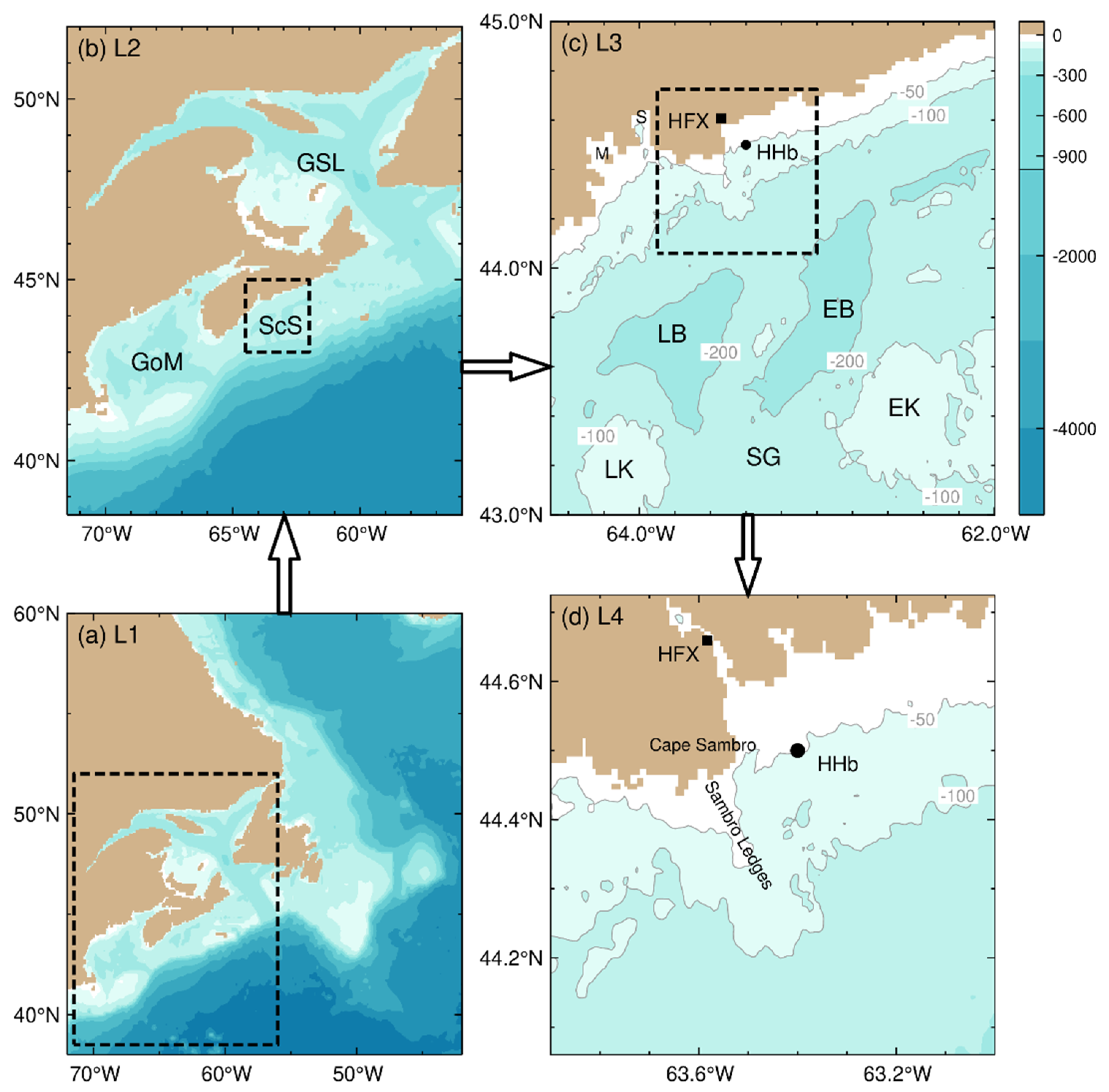
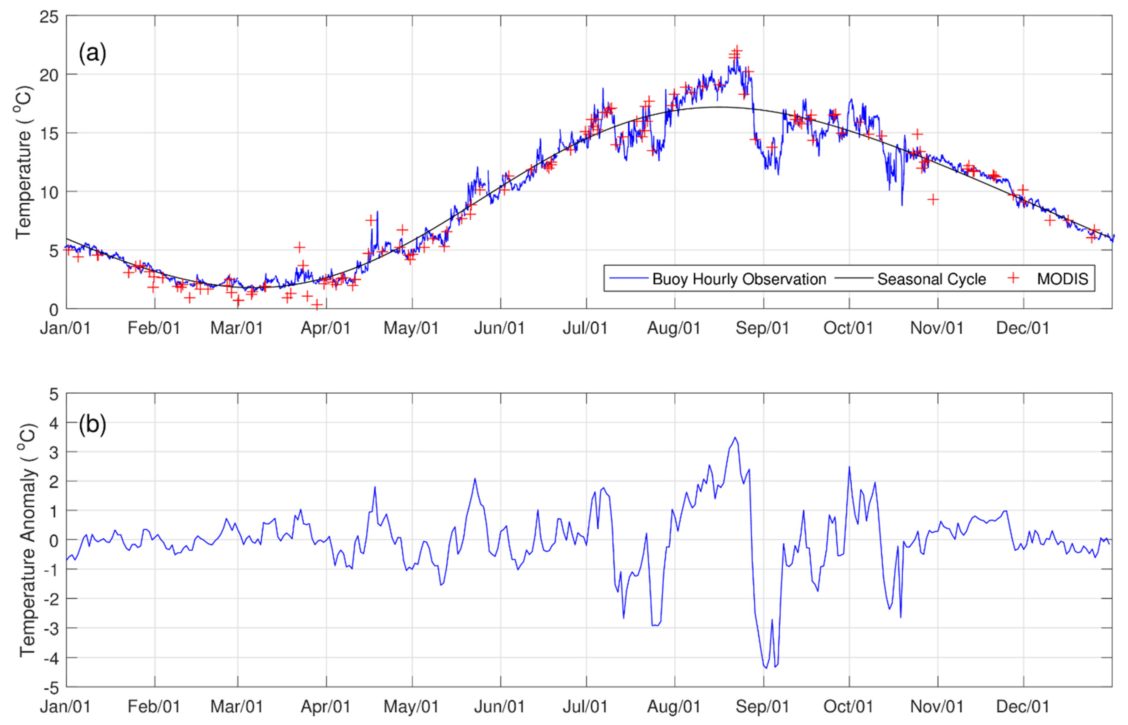
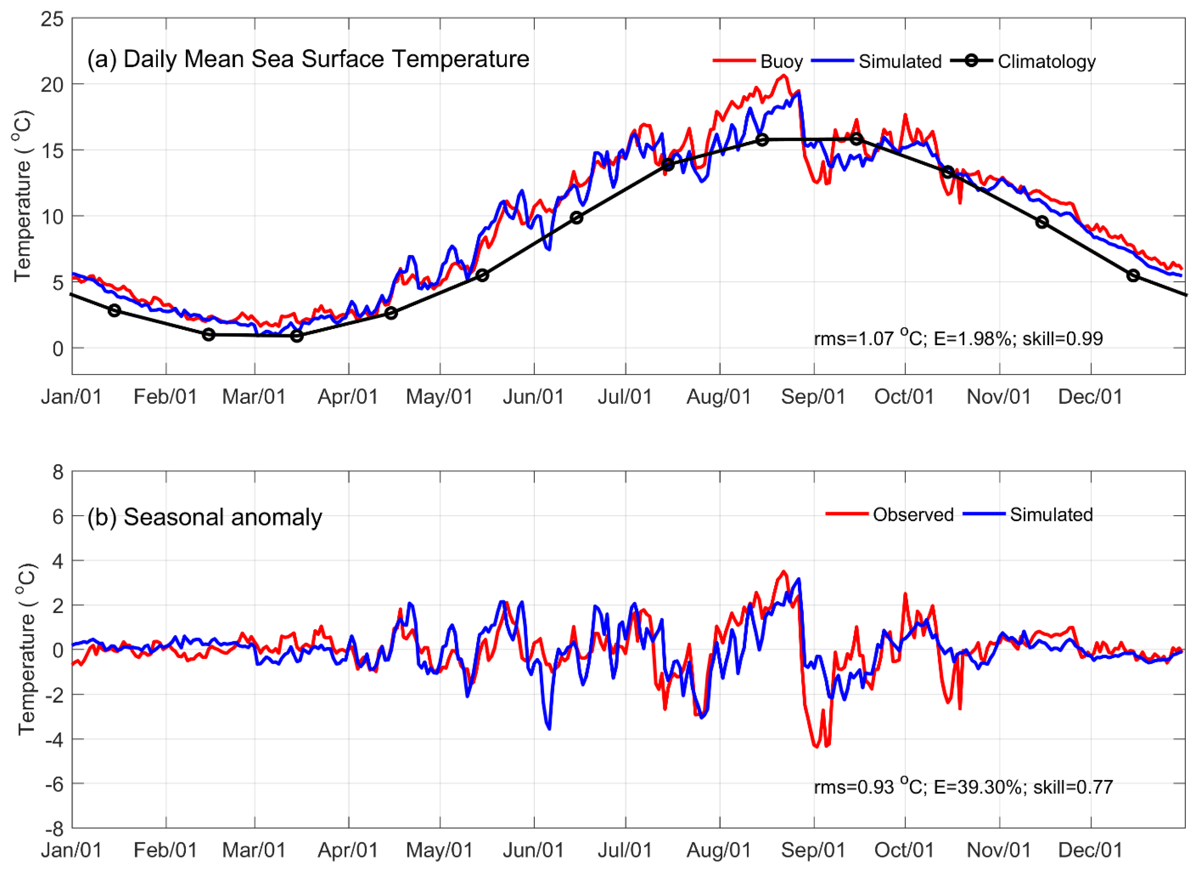
The simulated SSTs produced by submodel L3 of DalCoast-CSS are first compared with the in-situ observations made at location HHb outside Halifax Harbour (marked in Figure 1d). Figure 7a demonstrates that submodel L3 reproduces reasonably well the observed seasonal cycle of the SSTs at HHb, with the lowest value of simulated SSTs being about 2.0 °C at the beginning of March and the highest value being about 20.0 °C near the end of August in 2012 (Figure 7a). The lowest and highest values of SSTs at HHb produced by submodel L3 agree well with the in-situ observations. Figure 7a also presents the monthly mean SST climatology (black curve) at HHb calculated from hourly SST observations at this site for the 14-year period (2000–2013). The seasonal cycles of simulated and observed SSTs at HHb in 2012 are similar to each other, and both of them are warmer than the 14-year SST climatology.

To provide a quantitative measure of the model performance, we compute the following statistical measures [28]: the root-mean-square (rms) error defined as

$$rms=\sqrt{\frac{1}{N}{\sum }_{i=1}^N{\left(M-O\right)}^2}$$

(1)

the relative average error defined as

$$E=100\%\frac{{\sum }_{i=1}^N{\left(M-O\right)}^2}{{\sum }_{i=1}^N\left({\left(M-\overline{O}\right)}^2+{\left(O-\overline{O}\right)}^2\right)}$$

(2)

and the model skill parameter defined as

$$Skill=1-\frac{{\sum }_{i=1}^N{\left(M-O\right)}^2}{{\sum }_{i=1}^N{\left(\left|M-\overline{O}\right|+\left|O-\overline{O}\right|\right)}^2}$$

(3)

where $O$ and $M$ denote the observed and modelled variables respectively, $\overline{O}$ denotes the time mean of observed variable, and $N$ denotes the number of observations. For the skill parameter, perfect agreement between the model results and observations yields a skill of one, whereas complete disagreement yields a skill of zero. The values of $rms$ and $E$ are relatively small for the daily mean time series of SSTs, and the skill parameter is close to 1 (Figure 7a), indicating that submodel L3 performs well in simulating the daily mean observed SSTs at HHb.

Submodel L3 is also able to reproduce very well the high-frequency (weather-band) variability of observed SSTs, particularly during the wind-driven upwelling events, with the $rms$ = 0.93 °C, E = 39.3%, and the skill parameter equals 0.77 (Figure 7b). Both the observed and simulated SST anomalies at HHb have relatively small anomalies in winter, early spring and late fall seasons, and relatively large in late spring, summer, and early fall seasons in 2012 (Figure 7b). In particular, submodel L3 reproduces very well the observed SST anomalies during the upwelling events in July. The model also performs reasonably well in capturing the onset of the upwelling at the end of August. Submodel L3, however, underestimates the magnitude of the cooling of this upwelling event.

It should be noted that the four submodels of DalCoast-CSS are prognostic without data assimilation of real-time observations. The small rms errors for both the daily mean time series and seasonal anomalies of simulated SSTs indicate that the net heat flux calculation, vertical mixing parameterization, coastal currents, and advection of different water masses around HHb are satisfactory and adequate in the nested-grid modelling system.

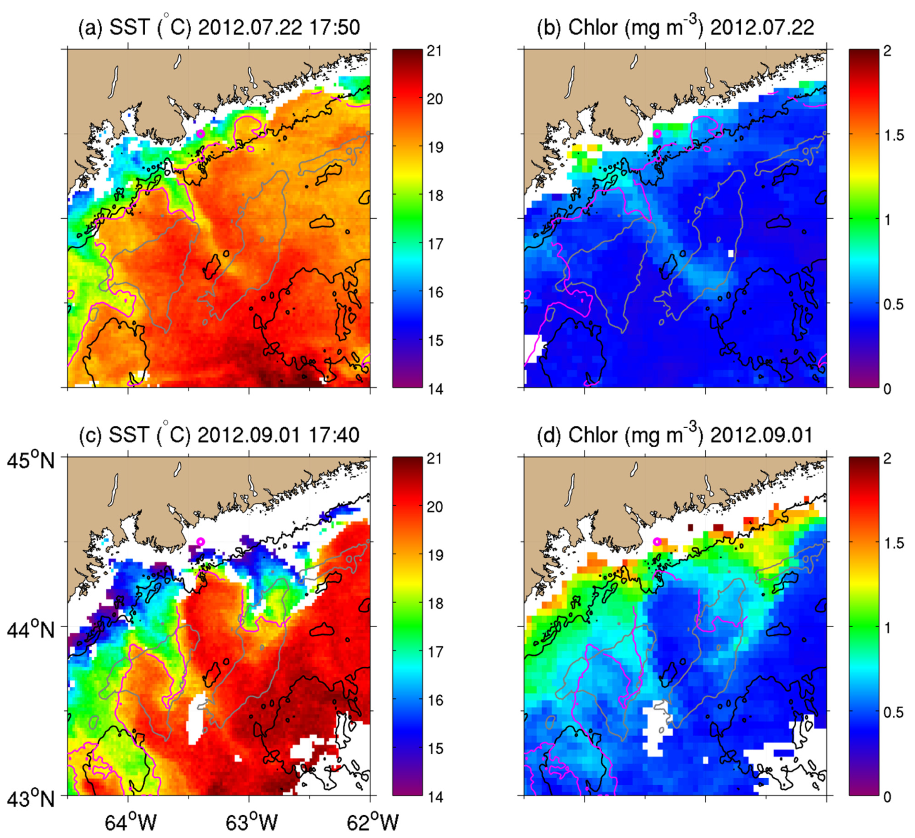
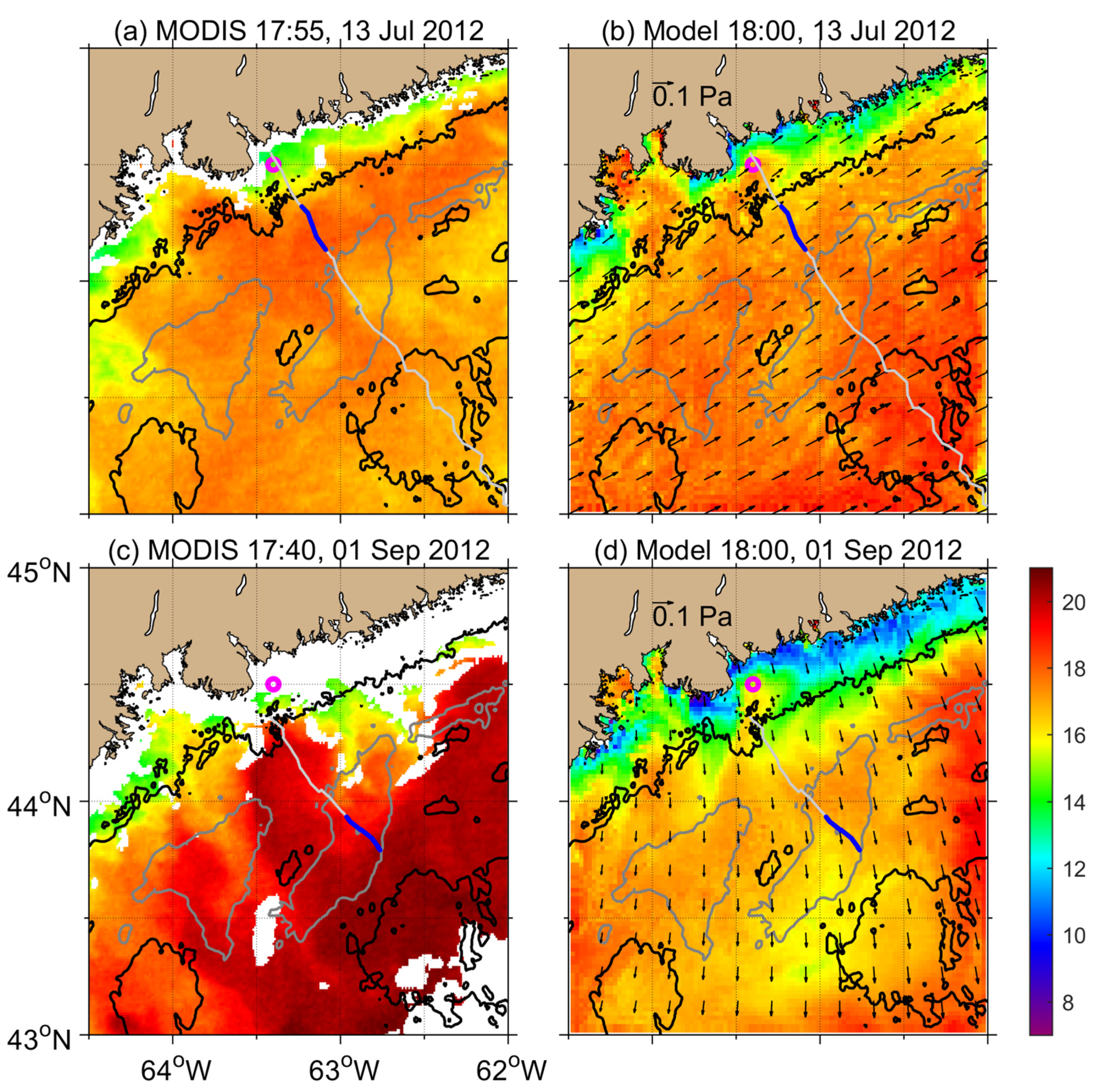
We next examine the performance of submodel L3 of DalCoast-CSS in reproducing the observed spatial variations of SSTs. Figure 8 presents a comparison of simulated SSTs with MODIS SST data over the central ScS at two specific times with relatively cloud-free conditions associated with the first and third major upwelling events in summer 2012. At 18:00 on 13 July 2012, the general horizontal patterns of the simulated coastal upwelling plume near the coast of Nova Scotia agree very well with satellite remote sensing SST data. The model also reproduces the along-shore variability of observed SSTs, particularly relatively warm SSTs in St. Margarets Bay, Mahone Bay, and adjacent coastal waters (Figure 8a,b). In the offshore deep waters of the central ScS, the simulated SSTs agree with the satellite SST data, which are relatively uniform and warm (>15 °C). As mentioned above, the circulation model is not data assimilative of real-time observations; thus, it is beyond the ability of the current version of the circulation model with the present spatial resolution to reproduce the cold water plume exactly at the observed locations. Therefore, the fact that the similar large-scale features in both the model results and remote sensing data indicates again the satisfactory model performance of submodel L3 of DalCoast-CSS.

Figure 8d demonstrates that at 18:00 on 1 September 2012, submodel L3 generates a broad band of cold waters over coastal waters of the central ScS due to persistent upwelling-favorable winds in late August. At this time, the MODIS satellite SST data are not available over most of the coastal waters of the central ScS. Nevertheless, some limited SST data available over coastal waters at this time confirm the broad band of cold waters near the coast associated with intensive coastal upwelling induced by winds (Figure 8c). In the deep offshore waters of the central ScS, the simulated SSTs at this time are relatively uniform, but cooler than the satellite SSTs. It should be noted that Submodel L3 performs less well in simulating the observed filaments. Only small filaments are developed along the 100 m isobath in the model, in comparison with observed filaments extending ~100 km offshore (Figure 8c,d). As stated above, it is a great challenge for a circulation model with the present spatial resolution to reproduce well the nonlinear instability of the observed cold upwelling plume. The other plausible reason is that the vertical and horizontal mixing in the model may be too large, which erodes the upwelling front and prevent the further growth of filaments.

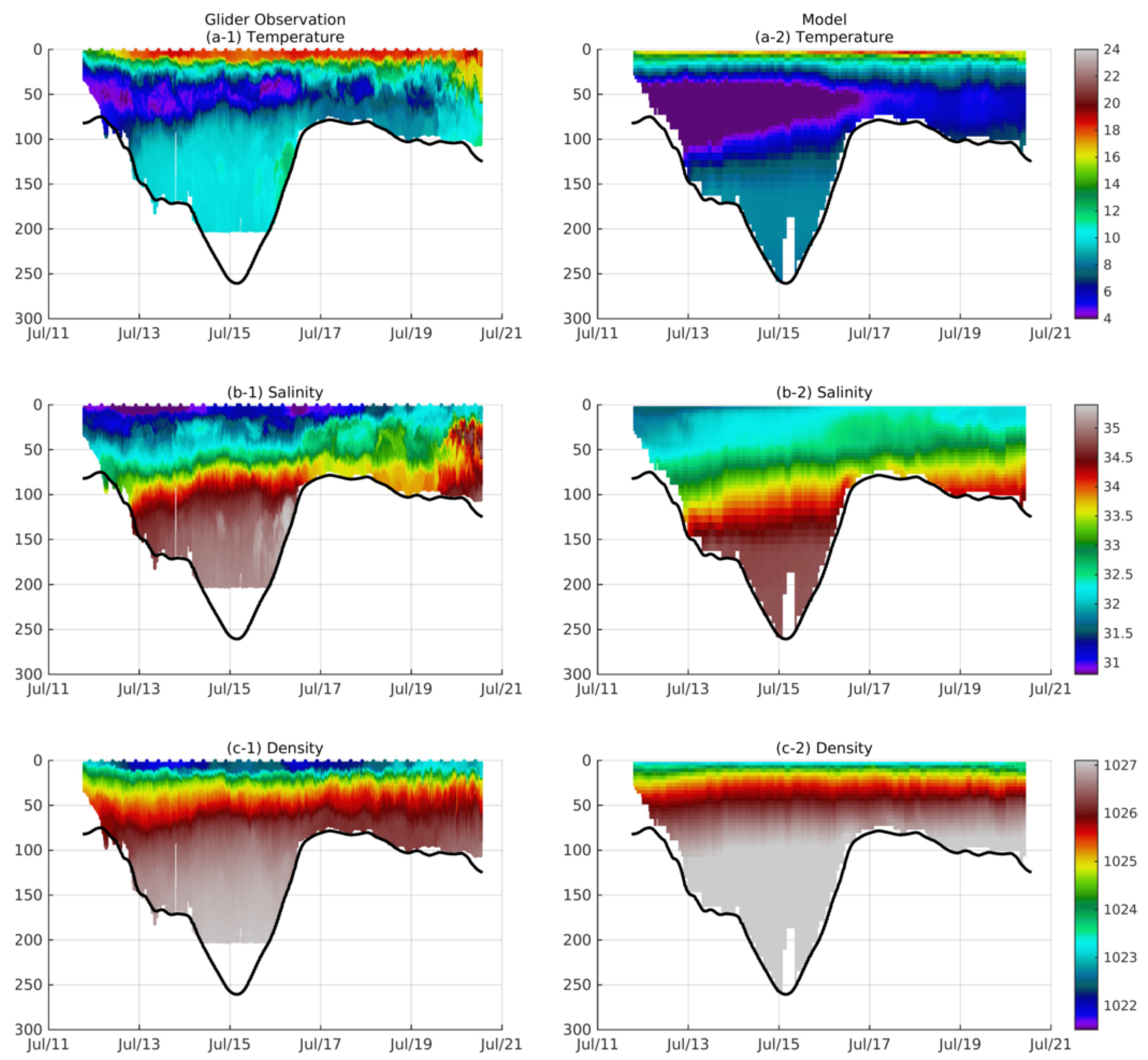
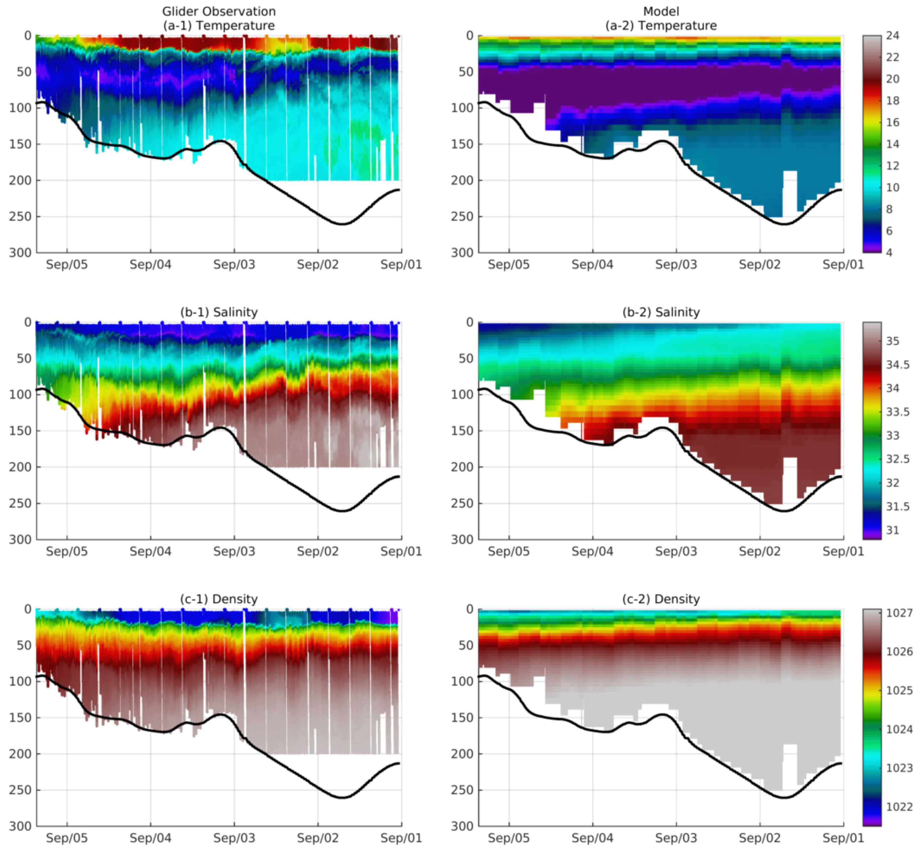
To demonstrate the model performance in simulating vertical stratification, we compare vertical distributions of the simulated hydrography by submodel L3 along two cross-shelf transects with in-situ observations made by a glider on 13 July and 1 September, respectively, during the first and third major coastal upwelling events in summer 2012 (Figure 9 and Figure 10). The glider track is shown in Figure 8. A comparison of vertical distributions of simulated and observed temperatures shown in Figure 9 and Figure 10 demonstrates that DalCoast-CSS reproduces reasonably well the observed three-layer structure in the vertical with a cold intermediate layer (CIL) occurring at depths between about 25 and 100 m in summer months. The formation of the CIL is mainly due to winter convection, wind-driven mixing in the previous winter and advection of upstream cold high-latitude water by the Nova Scotia Current [29]. It should be noted that the simulated warm surface layer is too thin and the CIL is too thick in the model in comparison with the glider observations. The thick CIL in the model could be related to the insufficient warm Slope Water intrusion at the shelf break in the model, which is likely due to the climatological open boundary conditions of temperature, salinity and currents specified in submodel L2. The thick CIL in turn reduces the thickness of the warm surface layer in the model through vertical mixing. The other possible reason is that the model resolution is too coarse to resolve the glider observed small-scale and high-frequency vertical variability along the thermocline.

A comparison of simulated and observed salinity distributions shown in Figure 9 and Figure 10 demonstrates that submodel L3 also reproduces reasonably well the relatively low salinity water associated with the Nova Scotia Current in the top 100 m and the relatively high salinity (>34.5) water in the deep layer (>100 m) of the Emerald Basin. However, the submodel L3 overestimates the salinity in the top 50 m, which could be explained by (1) the lack of freshwater input from small local rivers along the coast of Nova Scotia, and (2) the simple treatment of precipitation and evaporation processes at the sea surface in DalCoast-CSS. Figure 9 demonstrates that the simulated isopycnals tilt upward towards the coast (Figure 9(c-2)), which is similar to the observations (Figure 9(c-1)) during the major upwelling events in July. The upward tilted isopycnals are a direct result of the secondary circulation associated with coastal upwelling, which brings deeper denser water masses up to shallower areas.

4.2. Model Results during Upwelling/Downwelling Events

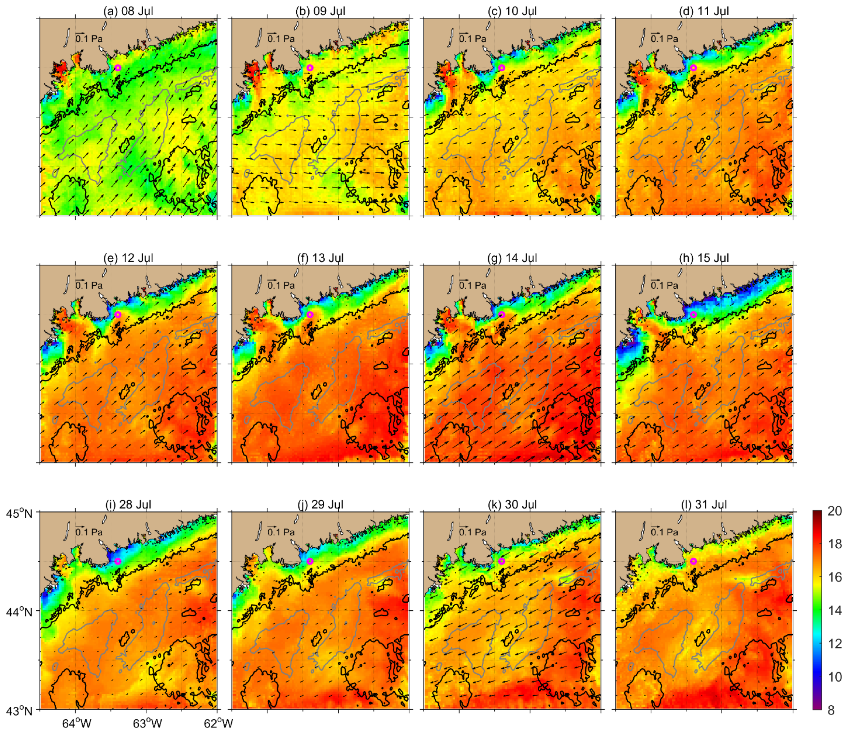
Figure 11 presents distributions of instantaneous SSTs produced by submodel L3 of DalCoast-CSS at 12 different times during the major upwelling/downwelling events in July 2012. For the first coastal upwelling event from 8 to 11 July 2012 (top panels of Figure 11), the along-shore winds during this period are upwelling-favorable (black arrows, Figure 11a). The SSTs produced by submodel L3 are relatively uniform and about 14 °C over the middle and outer ScS (beyond the 100-m isobath along the coastline), except for 16 °C over some isolated areas. The simulated SSTs during this 4-day period increase from about 15 °C to 18 °C due to the positive net heat flux at the sea surface from the atmosphere to the ocean. On 8 July, the SSTs near the coast (from coastline to the 100 m isobath) are relatively uniform and about 15 °C, which is similar to the SSTs on the Shelf. On 9 July, relatively low SSTs occur over two coastal areas: one is to the west of Halifax Harbour and the other to the west of Mahone Bay. In the next two days (10 and 11 July), the simulated SSTs over these two coastal areas further decrease to less than 10 °C. In addition, relatively low SSTs also occur over the coastal area to the northeast of Halifax Harbour in these two days (Figure 11c,d). 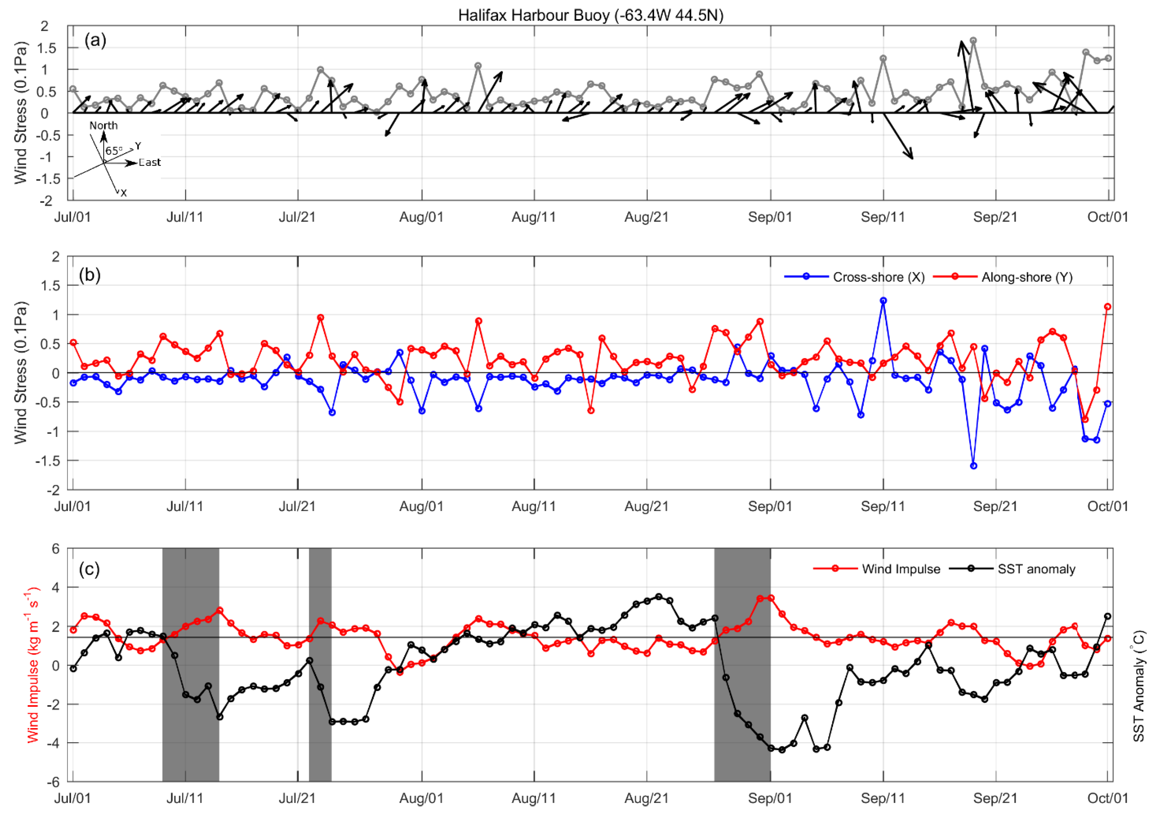From 12 to 15 July (middle panels of Figure 11), the wind forcing is mainly southwesterly (upwelling-favorable) and the wind impulse is peaked on 14 July (Figure 5c), leading to continuous development of coastal upwelling and significant offshore expansions of the low SST waters from coastal areas. It should be noted that the coastal upwelling plumes are not evident in St. Margarets Bay and Mahone Bay, indicating that the spatially varying development of coastal upwelling plume in the along-shore direction due to effects of local topography and coastline [30], even though the wind forcing is spatially uniform during this period (Figure 11e–h).

The bottom panels of Figure 11 present the simulated SSTs and wind vectors during a downwelling event from 28 to 31 July. Significant upwelling cold water plume occurs on 28 and 29 July over the inner ScS, except for slightly warmer SSTs in St. Margarets Bay and Mahone Bay and adjacent coastal waters (Figure 11i,j). On 30 July, the surface wind forcing used in DalCoast-CSS is mainly northeasterly (downwelling-favorable). The low SST areas near the coast are decreased under downwelling-favorable winds (Figure 11k) and the SSTs near the coast are relatively uniform on 31 July except for coastal waters (Figure 11l).

The general patterns of wind-driven coastal upwelling and downwelling near the coast of Nova Scotia shown in Figure 11 are qualitatively consistent with previous studies (e.g., [4]). In addition, the model is also able to capture the along-shore variations of the simulated SSTs using the relatively spatially uniform reanalysis wind over the central ScS, with warmer waters in St. Margarets Bay and Mahone Bay, which will be examined in the following section.

4.3. Process Study: Role of Irregular Coastline and Rugged Bathymetry

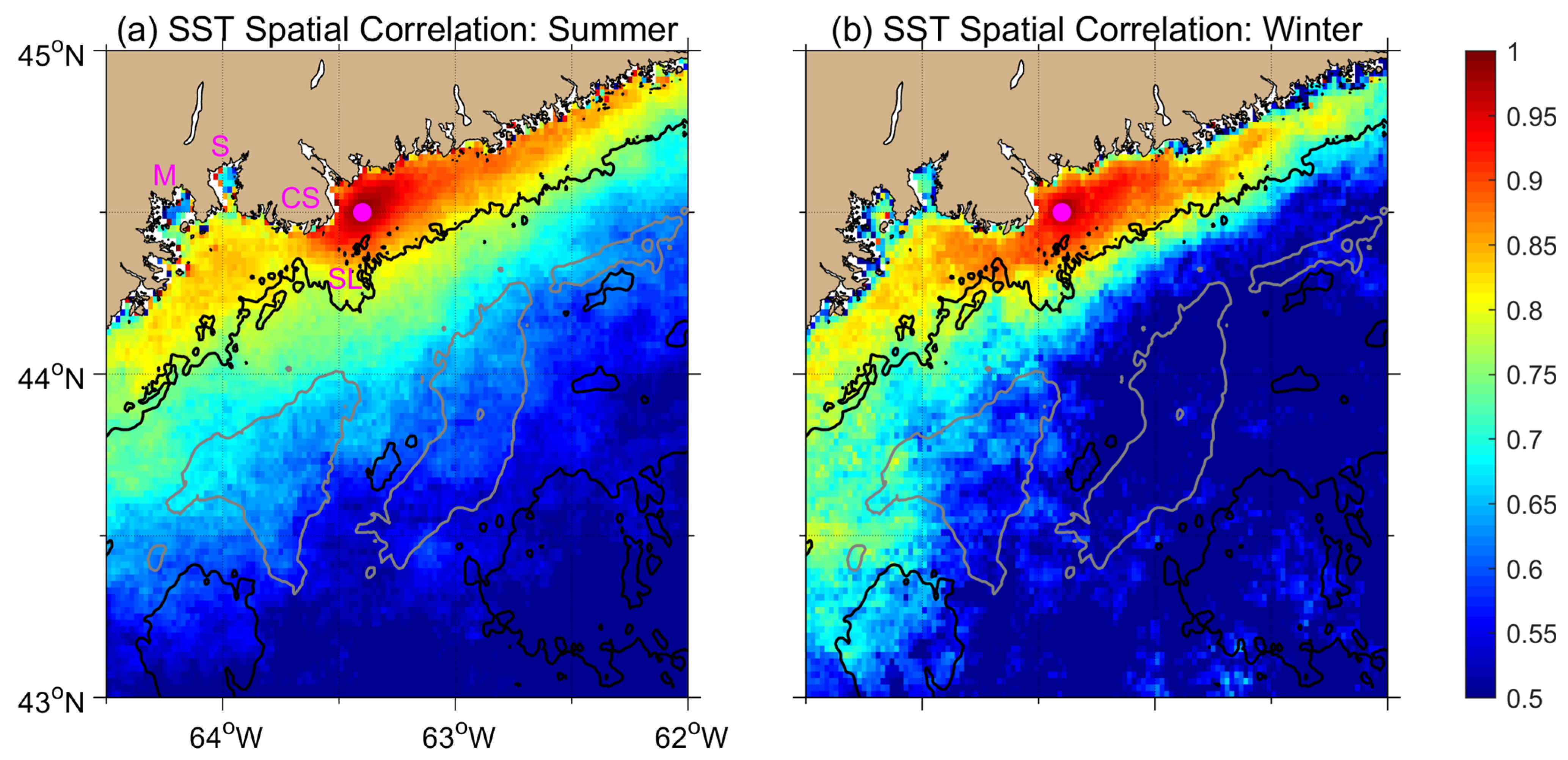
Model results and satellite SST observations discussed above demonstrate well that the wind-driven coastal upwelling over coastal waters of the central ScS has significant along-shore variability. In a theoretical study on the effects of topographic variations on coastal upwelling, Song and Chao [30] demonstrated that significant along-shore variation of upwelling fronts is caused by the combined effect of local topography and stratification. The correlation analysis of observed SSTs in summer presented in Section 3 (Figure 4) statistically shows a decorrelation of SSTs in St. Margarets Bay and Mahone Bay from the SSTs in the upstream. The simulated SST fields during a major coastal upwelling event in July 2012 (Figure 11) indicate that the surface waters in St. Margarets Bay and Mahone Bay are warmer than the adjacent coastal waters, which are consistent with the asymmetric pattern determined from the observational analysis.

There are significant bathymetric irregularities (i.e., Cape Sambro and Sambro Ledges) to the northeast (upstream) of St. Margarets Bay and Mahone Bay. To investigate the role of the irregular coastline and rugged bathymetry on the wind-driven coastal-upwelling over coastal waters of the central ScS, three additional numerical experiments are conducted using various specifications of coastline and nearshore bathymetry in submodel L3 of DalCoast-CSS:

• Experiment using constant wind forcing (UPwind): The DalCoast-CSS in this experiment is driven by the suite of forcing functions discussed in Section 2.2, including tides, river discharges, atmospheric forcing, and open boundary forcing, except that typical upwelling-favorable wind stress (0.05 Pa and 65°T) is specified in submodel L2 and L3.
• Experiment using straight coastline (UPline): Same as UPwind, except that the realistic irregular coastline in submodel L3 is replaced by a straight one.
• Experiment using smoothed topography (UPtopo): Same as UPwind, except that the realistic rugged bathymetry near the coast (e.g., Sambro Ledges, a submerged bank associated with Cape Sambro) in submodel L3 is replaced by a smoothed topography, in which the isobaths from 50 to 100 m adjacent to the coast are parallel to each other and have an angle of 65°T.

In these three additional experiments (i.e., UPwind, UPline and UPtopo), submodels L2 and L3 are initialized from the 3D circulation and hydrography fields produced by the realistic hindcast run on 30 June 2012. It should be noted that in UPtopo, topography smoothing in submodel L3 created a few model grids beyond the realistic maximum depth, and the temperature and salinity of those new grids are initialized by the near-bottom temperature and salinity from the realistic hindcast. Both L2 and L3 are integrated for one month. 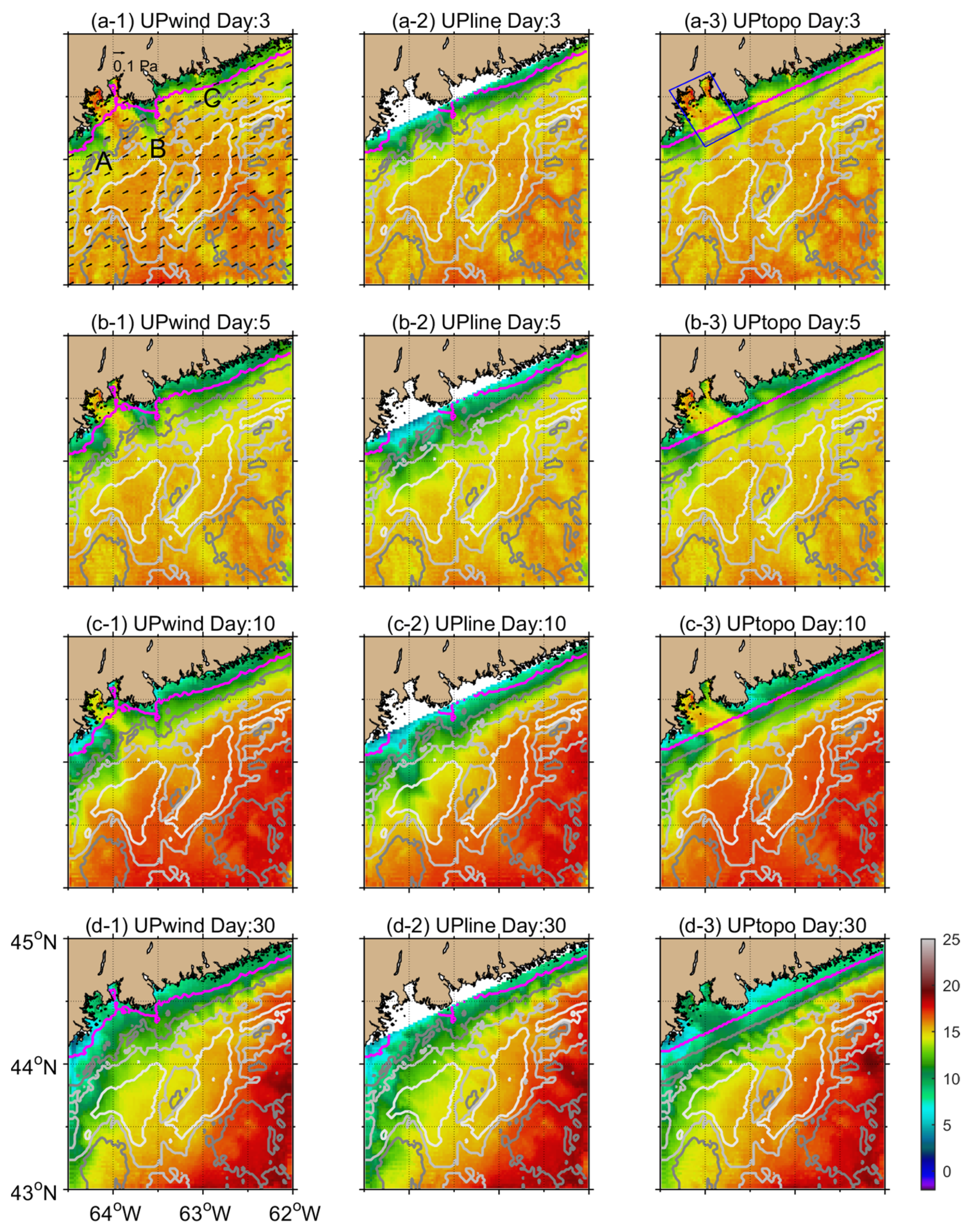The model results of SST and circulation fields at 3, 5, 10, and 30 days after 1 July 2012 in the three numerical experiments (Figure 12, Figure 13 and Figure 14) are examined to determine the effects of irregular coastline and rugged bathymetry on the coastal upwelling and associated spatial variability on the central ScS.

Model results in UPwind demonstrate that a coastal upwelling plume develops under the constant upwelling-favorable wind condition (left panels of Figure 12). After 3 days from the onset of the uniform wind forcing (Figure 12(a-1)), three filaments with relatively low SST waters are developed near the coast in the model, with one located to the west of Mahone Bay (Filament A, Figure 12(a-1)), one off the Cape Sambro (Filament B), and one at about 80 km to the northeast of Cape Sambro (Filament C). These three filaments extend about 50 km offshore on day 3. The SSTs to the northeast and southwest of Filament B are relatively warm and about 15 °C in this case. On day 5 (Figure 12(b-1)), the three filaments in UPwind are further extended offshore. On day 10 (Figure 12(c-1)), Filament A in UPwind is further extended offshore, and Filaments B and C are merged into a cold water band near the coast, and St. Margarets Bay is covered by relatively cold surface waters associated with the upwelling plume. The SST in Mahone Bay on day 10 is warmer than the SST inside the upwelling plume but colder than the SST on the Shelf. The SSTs over the middle and outer shelf increase from about 15 °C to 18 °C, mainly due to the positive surface heat flux from the overlying atmosphere to the ocean. On day 30 in UPwind (Figure 12(d-1)), Filament A is extended to LaHave Bank, and Mahone Bay is completely covered by relatively cold surface water associated with the upwelling plume. Backward breaking waves associated with the instability at the plume front [31] are evident along the 100 m isobath to the northeast of Sambro Ledges (Figure 12(d-1)). It should be noted that the steady along-shore wind for 30 days is an idealized extreme case and the associated widely-spread low SST water band over the inner ScS in Figure 12(d-1) is not very common on the ScS.

The coastal upwelling plume along a straight coastline produced by submodel L3 in UPline (middle panels of Figure 12) has several distinct features in comparison with the plume in UPwind. On day 3, three filaments are also evident along the straight coastline in UPline (Figure 12(a-2)). In comparison with the filaments in UPwind, the filaments in UPline extend further offshore. The filament close to Cape Sambro (Filament B) in UPline is located further southwest compared to the one in UPwind. On day 5 (Figure 12(b-2)), the filaments in UPline extend further offshore, and Filament B moves closer to Filament A, which is located to the west of Mahone Bay. On day 10, Filament B is merged with Filament A to form a larger filament (Figure 12(c-2)). Another filament is developed off Cape Sambro on day 10 (Figure 12(c-2)). On day 30, the upwelling plume is very similar to the plume in UPwind. Backward breaking waves associated with the instability at the plume front are also developed along the 100 m isobath to the northeast of Sambro Ledges (Figure 12(d-2)). The southwestward propagation of the filament from Cape Sambro in the straight coastline is not evident based on model results of UPwind, which indicates that the cape has a scattering effect for the along-shore wave propagation of the filaments.

The coastal upwelling plume in UPtopo, in which Sambro Ledges are removed, has similar features near the coast but distinct features in the offshore deep waters in comparison with the plume in UPwind. On day 3, 5, and 10, the coastal upwelling plume from the coast to the 50 m isobath in UPtopo is very similar to the plume in UPwind, indicating that the presence of Sambro Ledges has a minor effect on the initial development of the filaments near the coast. On day 10, the cold upwelling plume is evident along the coast except for the areas outside St. Margarets Bay and Mahone Bay. At day 30, backward breaking waves associated with the instability at the plume front are developed along the 150 m isobath from northeast to southwest in UPtopo (Figure 12(d-3)), while the instability waves are disrupted by the presence of Sambro Ledges in UPwind (Figure 12(d-1)).

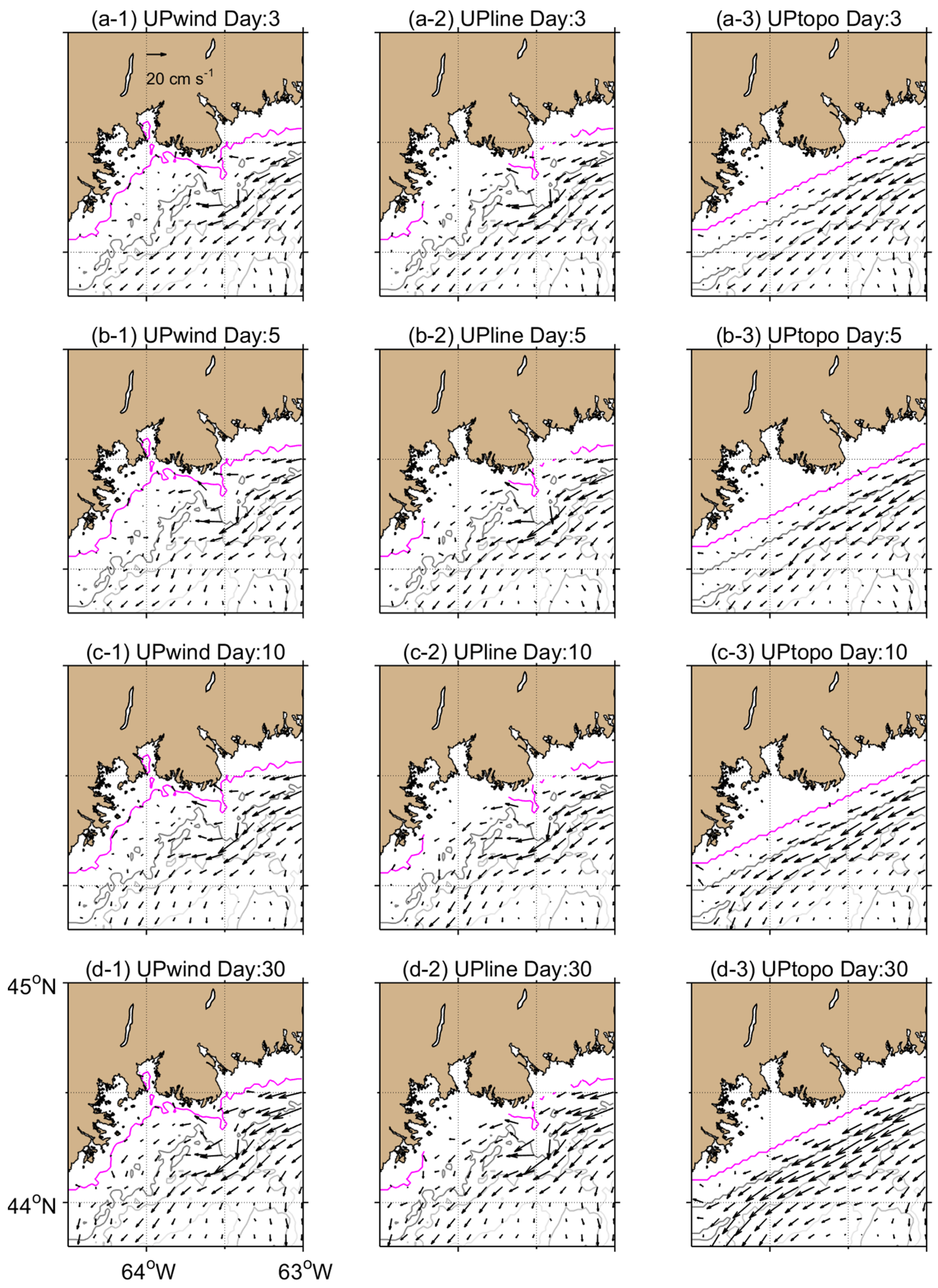
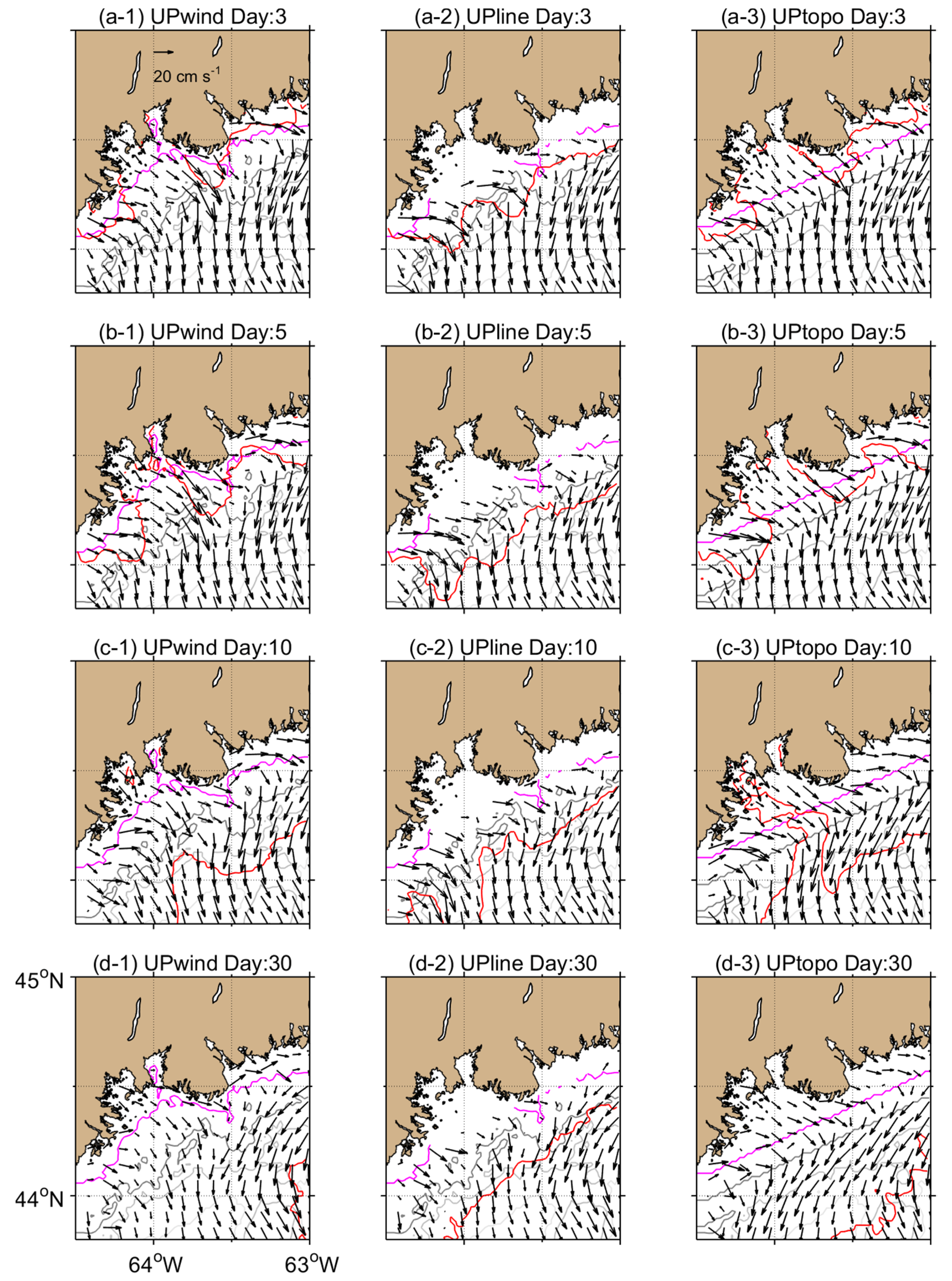
In addition to the SST fields, the circulation fields adjacent to Sambro Ledges at two depths (near-surface and ∼50 m) in three additional experiments are also examined (Figure 13 and Figure 14). For the near-surface circulation on day 3 in UPwind two regimes are evident from the coast to the middle shelf of the central ScS. The first regime is the coastal region with the local water depths less than 50 m. In this region, the near-surface currents are eastward or southeastward mainly due to the upwelling-favorable wind forcing. The second regime is the offshore region beyond the 50 m isobath. Over this region, the currents are significantly modified by the southwestward buoyancy-driven Nova Scotia Current. In UPwind on day 3 and 5, a relatively strong offshore current associated with the edge of the upwelling plume (12 °C isotherm in Figure 13(a-1),(b-1)) occurs in the lee of Sambro Ledges. On day 10 and 30, the currents in the lee of Sambro Ledges are reduced as the edge of the upwelling plume moves further offshore. In UPline, the relatively strong offshore currents in the lee of Sambro Ledges are not evident during the 30-day period. In UPtopo, the Nova Scotia Current on day 10 and 30 penetrates further to the southwest due to the absence of Sambro Ledges. For the circulation at 50 m (Figure 14), the influence of Sambro Ledges is more evident compared to the near-surface circulation fields (Figure 13). In these three additional experiments, the main subsurface circulation feature is the Nova Scotia Current, which flows southwestward following the 150 m isobath along the coast. In UPwind and UPline, offshore and onshore flows are evident to the northeast and southwest of Sambro Ledges due to local topographic steering. In UPtopo, however, the Nova Scotia Current is not deflected since Sambro Ledges are removed, and the currents to the southwest (downstream) of Sambro Ledges are relatively stronger in UPtopo than the currents in UPwind.

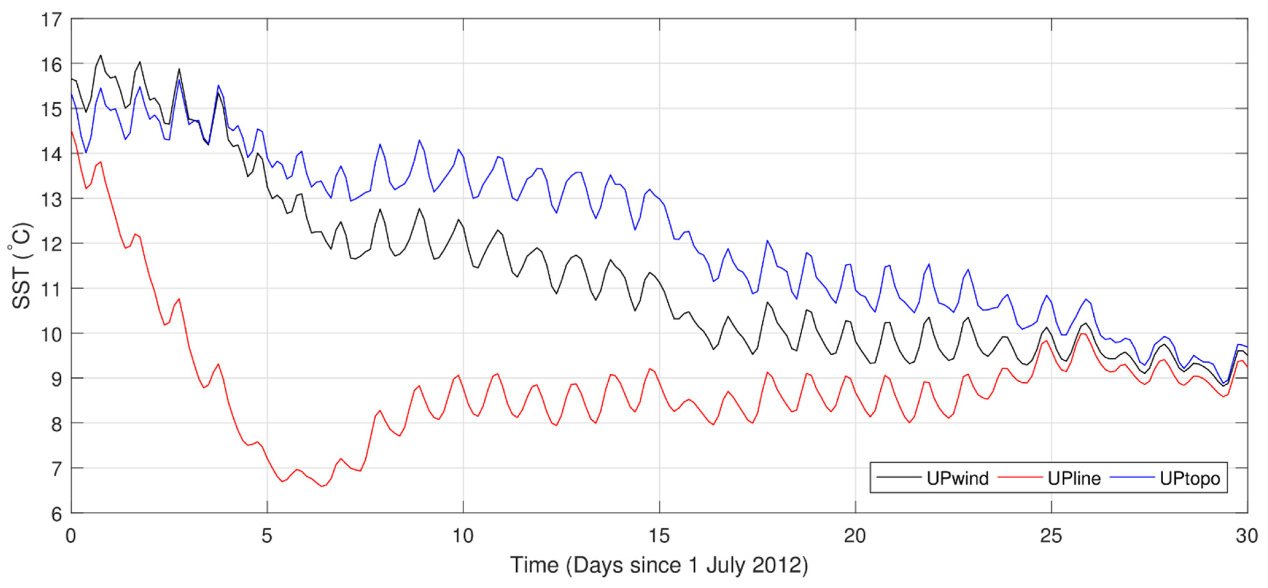
We next examine the temporal variability of area-averaged SSTs over St. Margarets Bay, Mahone Bay, and adjacent coastal waters (Figure 15) in the three additional numerical experiments. The diurnal surface heating is evident in these three experiments. The sub-diurnal SST responses can be categorized into two periods: (1) the initial response period (first 4 days) and (2) the continued response period (after 4 days). It should be noted that the time-scale of the initial response (∼4 days) in these three experiments is comparable to the initial response period of a typical realistic upwelling-favorable wind event (gray vertical bars in Figure 5c). In UPwind, initially the area-averaged SSTs oscillate around 15.5 °C. After day 4, the area-averaged SSTs decrease with time to ∼9.5 °C on day 30. In UPline, the area-averaged SSTs are significantly different from the SSTs in UPwind during the 30-day period. The sub-diurnal SSTs in UPline feature a rapid linear drop from 14.5 °C to ∼7 °C during the first 5 days and a gradual increase to about ∼9.5 °C during the following 25 days. In UPtopo, the area-averaged SSTs are only significantly different from the SSTs in UPwind during the continued response period. The temperature difference between UPtopo and UPwind increases from nearly 0 at day 4 to a maximum of ~2 °C on day 15, and then decreases to ~0.2 °C on day 30. The effect of irregular coastline and rugged bathymetry on the time-dependent response of SSTs during upwelling events can be summarized as follows. First, the differences (similarities) of SSTs in UPwind and UPline (UPtopo) in the initial response period support the idea that the irregular coastline is the main controlling factor for the observed relatively warm SSTs in St. Margarets Bay and Mahone Bay during the initial response period. Secondly, the similarities and differences of SSTs in UPwind and UPtopo in the initial and continued response periods, respectively, suggest that the small-scale rugged bathymetry has less effect on the SST variation in the initial response period, but plays an important role in the SST variations in the continued response period. Lastly, the results from the three experiments also suggest that the influence of irregular coastline and rugged bathymetry on the SSTs in the two Bays is reduced towards the end of the month, at which time the upwelling plume has been fully-developed.

5. Summary and Conclusions

The temporal and spatial variability of coastal upwelling during three major upwelling events in summer 2012 over the central Scotian Shelf (ScS) was examined based on in-situ and remote sensing observations and model results produced by a nested-grid ocean circulation model (DalCoast-CSS). The analysis of satellite remote sensing observations of sea surface temperatures (SSTs) demonstrated large spatial and temporal variabilities in the SSTs during upwelling events with relatively cold water bands along the coast and filaments extending offshore. A spatial correlation analysis of the observed SSTs showed an asymmetry due to a coastal irregularity (i.e., Cape Sambro) with smaller correlation coefficients in the downstream area during upwelling seasons. A regression analysis indicated that the wind impulse plays a major role in controlling the SST variations during the initial response period of the upwelling events.

The SST variations associated with the upwelling plume were further studied by using a nested-grid circulation model driven by a suite of external forcing and with realistic coastline and topography (control run, CR). Submodel L3 of DalCoast-CSS in CR is able to reproduce reasonably well the temporal and spatial variability of observed SSTs, particularly during the wind-driven upwelling events in July 2012. Although, the model captures the onset of the upwelling at the end of August, it underestimates the magnitude of the cooling of this upwelling event. Many factors could contribute to the model bias. Taking the surface boundary condition as an example, the energy and momentum fluxes in the ocean model do not fully account for the impact of oceanic waves at the air-sea interface [32]. Typically the atmosphere circulation model, ocean surface wave model, and ocean circulation model are run independently of each other. Thus, the ocean surface wave influence on the wind-driven coastal upwelling has rarely been investigated. A recent study suggested that the inclusion of wave effects could further improve the model performance in simulating the coastal upwelling along the Swedish coast [33]. A next step in terms of DalCoast-CSS model development is to examine the wave effects on the wind-driven coastal upwelling on the Scotian Shelf by using a fully coupled atmosphere-wave-ocean modelling system.

The roles of irregular coastline and rugged bathymetry in coastal upwelling were investigated based on model results from three additional numerical experiments, which differ from the CR only in the specification of coastline and nearshore bathymetry and wind forcing. It was demonstrated that irregular coastline (e.g., cape) is responsible for the relatively warm SST in St. Margarets Bay and Mahone Bay, which are located in the downstream direction of Cape Sambro, and small-scale rugged bathymetry (e.g., submerged bank) steers the circulation in its adjacent area and downstream, thus influences the spatial extend of filaments through advection process.

In addition to the effect on the temperature and circulation fields, the small-scale bathymetric irregularities can indirectly influence the coastal dynamics and ecosystem [34]. The distinct time-dependent SST response to upwelling-favorable winds in St. Margarets Bay and Mahone Bay should be taken into account when interpreting larval transport, settlement, and abundance of temperature-sensitive species in the Bays; and comparing the ecosystem in the Bays with adjacent coastal areas [23].

The important new findings and modelling approach used in the present study of coastal upwelling on the Scotian Shelf are expected to be applicable to other coastal regions worldwide, because the general upwelling patterns and dynamic principles [5] are common to all coastal regions where wind-driven upwelling occurs [1]. The major influence of small-scale bathymetric irregularities discussed in this study suggests that high-resolution circulation and ecosystem models sufficiently resolving the coastline and nearshore bathymetry are needed to properly capture the evolution of the coastal upwelling plume and associated nutrient and larval transport.

References

1. Kämpf, J.; Chapman, P. Upwelling Systems of the World; Springer: Berlin/Heidelberg, Germany, 2016. [Google Scholar]
2. Hu, J.; San Liang, X.; Lin, H. Coastal Upwelling off the China Coasts. In Coastal Environment, Disaster, and Infrastructure-A Case Study of China’s Coastline; IntechOpen: London, UK, 2018; pp. 3–25. [Google Scholar]
3. Moore-Maley, B.; Allen, S.E. Wind-Driven Upwelling and Surface Nutrient Delivery in a Semi-Enclosed Coastal Sea. Ocean Sci. 2022, 18, 143–167. [Google Scholar] [CrossRef]
4. Petrie, B.; Topliss, B.J.; Wright, D.G. Coastal Upwelling and Eddy Development off Nova Scotia. J. Geophys. Res. Ocean. 1987, 92, 12979–12991. [Google Scholar] [CrossRef]
5. Ekman, V.W. On the Influence of the Earth’s Rotation on Ocean-Currents; Almqvist & Wiksells Boktryckeri AB: Uppsala, Sweden, 1905. [Google Scholar]
6. Hachey, W. Ekman’s Theory Applied to Water Replacements on the Scotian Shelf. Proc. Nova Scotian Inst. Sci. 1937, 19, 1934–1938. [Google Scholar]
7. Donohue, S.M. A Numerical Model of an Upwelling Event off the Coast of Nova Scotia. Master’s Thesis, Royal Military College of Canada, Kingston, ON, Canada, 2001. [Google Scholar]
8. Laurent, A. Examining the Influence of Meteorological Events on Plankton Dynamics in a Coastal Ecosystem (Lunenburg Bay, Canada). Ph.D. Thesis, Dalhousie University, Halifax, NS, Canada, 2011. [Google Scholar]
9. Thompson, K.; Loucks, R.; Trites, R. Sea Surface Temperature Variability in the Shelf-Slope Region of the Northwest Atlantic. Atmos. Ocean 1988, 26, 282–299. [Google Scholar] [CrossRef] [Green Version]
10. Donlon, C.; Minnett, P.; Gentemann, C.; Nightingale, T.; Barton, I.; Ward, B.; Murray, M. Toward Improved Validation of Satellite Sea Surface Skin Temperature Measurements for Climate Research. J. Clim. 2002, 15, 353–369. [Google Scholar] [CrossRef] [Green Version]
11. Dever, M.; Hebert, D.; Greenan, B.J.W.; Sheng, J.; Smith, P.C. Hydrography and Coastal Circulation along the Halifax Line and the Connections with the Gulf of St. Lawrence. Atmos. Ocean 2016, 54, 199–217. [Google Scholar] [CrossRef]
12. Shan, S.; Sheng, J.; Ohashi, K.; Dever, M. Assessing the Performance of a Multi-Nested Ocean Circulation Model Using Satellite Remote Sensing and in-situ Observations. Satell. Oceanogr. Meteorol. 2016, 1, 39–59. [Google Scholar] [CrossRef]
13. Mellor, G.L. Users Guide for a Three Dimensional, Primitive Equation, Numerical Ocean Model; Atmospheric and Oceanic Sciences Program, Princeton University: Princeton, NJ, USA, 2004. [Google Scholar]
14. Sheng, J.; Wright, D.G.; Greatbatch, R.J.; Dietrich, D.E. CANDIE: A New Version of the DieCAST Ocean Circulation Model. J. Atmos. Ocean. Technol. 1998, 15, 1414–1432. [Google Scholar] [CrossRef]
15. Mesinger, F.; DiMego, G.; Kalnay, E.; Mitchell, K.; Shafran, P.C.; Ebisuzaki, W.; Jović, D.; Woollen, J.; Rogers, E.; Berbery, E.H.; et al. North American Regional Reanalysis. Bull. Am. Meteorol. Soc. 2006, 87, 343–360. [Google Scholar] [CrossRef] [Green Version]
16. Gill, A.E. Atmosphere-Ocean Dynamics; Academic Press: Cambridge, MA, USA, 1982; Volume 30. [Google Scholar]
17. Ohashi, K.; Sheng, J. Influence of St. Lawrence River Discharge on the Circulation and Hydrography in Canadian Atlantic Waters. Cont. Shelf Res. 2013, 58, 32–49. [Google Scholar] [CrossRef]
18. Egbert, G.D.; Erofeeva, S.Y. Efficient Inverse Modeling of Barotropic Ocean Tides. J. Atmos. Ocean. Technol. 2002, 19, 183–204. [Google Scholar] [CrossRef] [Green Version]
19. Urrego-Blanco, J.; Sheng, J. Interannual Variability of the Circulation over the Eastern Canadian Shelf. Atmos. Ocean 2012, 50, 277–300. [Google Scholar] [CrossRef] [Green Version]
20. Thompson, K.R.; Ohashi, K.; Sheng, J.; Bobanovic, J.; Ou, J. Suppressing Bias and Drift of Coastal Circulation Models through the Assimilation of Seasonal Climatologies of Temperature and Salinity. Cont. Shelf Res. 2007, 27, 1303–1316. [Google Scholar] [CrossRef]
21. Sheng, J.; Greatbatch, R.J.; Wright, D.G. Improving the Utility of Ocean Circulation Models through Adjustment of the Momentum Balance. J. Geophys. Res. Ocean. 2001, 106, 16711–16728. [Google Scholar] [CrossRef]
22. Huot, Y.; Babin, M.; Bruyant, F.; Grob, C.; Twardowski, M.; Claustre, H. Does Chlorophyll a Provide the Best Index of Phytoplankton Biomass for Primary Productivity Studies? Biogeosci. Discuss. 2007, 4, 707–745. [Google Scholar]
23. Saunders, M.; Metaxas, A. Temperature Explains Settlement Patterns of the Introduced Bryozoan Membranipora Membranacea in Nova Scotia, Canada. Mar. Ecol. Prog. Ser. 2007, 344, 95–106. [Google Scholar] [CrossRef] [Green Version]
24. Haidvogel, D.B.; Beckmann, A.; Hedström, K.S. Dynamical Simulations of Filament Formation and Evolution in the Coastal Transition Zone. J. Geophys. Res. Ocean. 1991, 96, 15017–15040. [Google Scholar] [CrossRef]
25. Røed, L.P.; Shi, X.B. A Numerical Study of the Dynamics and Energetics of Cool Filaments, Jets, and Eddies off the Iberian Peninsula. J. Geophys. Res. Ocean. 1999, 104, 29817–29841. [Google Scholar] [CrossRef]
26. Large, W.; Pond, S. Open Ocean Momentum Flux Measurements in Moderate to Strong Winds. J. Phys. Oceanogr. 1981, 11, 324–336. [Google Scholar] [CrossRef] [Green Version]
27. Cushman-Roisin, B.; Beckers, J.-M. Introduction to Geophysical Fluid Dynamics: Physical and Numerical Aspects; Academic Press: Cambridge, MA, USA, 2011. [Google Scholar]
28. Zhong, L.; Li, M. Tidal Energy Fluxes and Dissipation in the Chesapeake Bay. Cont. Shelf Res. 2006, 26, 752–770. [Google Scholar] [CrossRef]
29. Umoh, J.U.; Thompson, K.R. Surface Heat Flux, Horizontal Advection, and the Seasonal Evolution of Water Temperature on the Scotian Shelf. J. Geophys. Res. Ocean. 1994, 99, 20403–20416. [Google Scholar] [CrossRef]
30. Song, Y.T.; Chao, Y. A Theoretical Study of Topographic Effects on Coastal Upwelling and Cross-Shore Exchange. Ocean. Model. 2004, 6, 151–176. [Google Scholar] [CrossRef]
31. Griffiths, R.; Linden, P. The Stability of Buoyancy-Driven Coastal Currents. Dyn. Atmos. Ocean. 1981, 5, 281–306. [Google Scholar] [CrossRef]
32. Janssen, P.A. Wave-Induced Stress and the Drag of Air Flow over Sea Waves. J. Phys. Oceanogr. 1989, 19, 745–754. [Google Scholar] [CrossRef] [Green Version]
33. Wu, L.; Staneva, J.; Breivik, Ø.; Rutgersson, A.; Nurser, A.G.; Clementi, E.; Madec, G. Wave Effects on Coastal Upwelling and Water Level. Ocean Model. 2019, 140, 101405. [Google Scholar] [CrossRef]
34. Largier, J.L. Upwelling Bays: How Coastal Upwelling Controls Circulation, Habitat, and Productivity in Bays. Annu. Rev. Mar. Sci. 2020, 12, 415–447. [Google Scholar] [CrossRef]
Figure 1. Major bathymetric features of the Scotian Shelf and adjacent northwest Atlantic Ocean (a–d). In (c,d), the black solid circle indicates the position of a buoy in Halifax Harbour (HHb). Land is masked by the tan color. The 50 m, 100 m, and 200 m isobaths are shown by the gray contours. Unit in color bar is m. The Gulf of Maine (GoM), Scotian Shelf (ScS), Gulf of St. Lawrence (GSL) are labelled in (b). LaHave Basin (LB), LaHave Bank (LK), Emerald Basin (EB), Emerald Bank (EK) and Scotian Gulf (SG) are labelled in (c). The four panels represent the four submodels of the nested-grid ocean circulation model used in this study. The following geographical names are used in the discussion of coastal upwelling and labelled in (c,d): Mahone Bay (M), St.Margarets Bay (S), Halifax Harbour (HFX), Cape Sambro and Sambro Ledges.
Jmse 10 00497 g001
Figure 2. (a) Hourly time series of in-situ SSTs (blue) in 2012 and the fitted seasonal cycle (black) at location HHb outside Halifax Harbour. MODIS SSTs at location HHb are plotted as red “+”. (b) Time series of daily mean SST anomalies calculated by subtracting the seasonal cycle from the observed hourly SSTs in 2012.
Jmse 10 00497 g002
Figure 3. Satellite remote sensing data of sea surface temperature (SST) and chlorophyll concentration over the central Scotian Shelf and adjacent deep ocean waters on (a,b) 22 July and (c,d) 1 September, 2012. In (a,c), unit in color bar is °C. In (b,d), unit in color bar is mg m-3. SSTs were extracted from the Ocean Color Website (http://oceancolor.gsfc.nasa.gov (accessed on 22 March 2022)). Chlorophyll concentrations were extracted from the dataset provided by the Ocean Color Climate Change Initiative project (http://www.oceancolour.org (accessed on 22 March 2022)). The position marked by “◦” indicates the location of the Halifax Harbour buoy (HHb). The 18.5 °C isotherm is shown by magenta contours. The 100 m and 200 m isobaths are marked by the black and gray contours, respectively. White areas indicate missing remote sensing data due to cloud coverage and land contamination.
Jmse 10 00497 g003
Figure 4. Distributions of spatial correlation coefficients of MODIS SSTs over the central Scotian Shelf in relation to the SST at location HHb in (a) summer and (b) winter. MODIS SSTs from 2002 to 2014 were used in the calculation. The position marked by “◦” indicates the location of HHb. The 100 m and 200 m isobaths are marked by the black and gray contours, respectively. The small-scale bathymetric features of Cape Sambro (CS) and Sambro Ledges (SL) are labelled in (a). Mahone Bay (M) and St. Margarets Bay (S) are also marked in (a).
Jmse 10 00497 g004
Figure 5. (a) Daily mean wind stress (black arrows) and the magnitude of wind stress (gray line), (b) along-shore (65°T, red line) and cross-shore (blue line) components of wind stress, and (c) wind impulse (kg m−1 s−1, red line) and SST anomaly (°C, black line) in July, August and September 2012 at location HHb. In (c), the gray vertical bars indicate the initial response periods of three major upwelling events. The time-mean wind impulse in July, August, and September 2012 is ~1.4 kg m−1 s−1 as shown by the horizontal black line in (c).
Jmse 10 00497 g005
Figure 6. Scatterplot between wind impulse anomaly and SST anomaly in July, August, and September 2012 at location HHb. The wind impulse anomaly is calculated by subtracting the time-mean wind impulse from the daily wind impulse. The time-mean wind impulse is ~1.4 kg m−1 s−1 as shown by the horizontal black line in Figure 5c. The values during the initial response periods (gray vertical bars in Figure 5c) are shown in red solid circles. The correlation coefficient (R) is equal to −0.86 for the solid circles. The linear regression lines are shown.
Jmse 10 00497 g006
Figure 7. Daily mean time series of (a) observed (red) and simulated (blue) SSTs and (b) seasonal SST anomalies at location HHb in 2012. The simulated results are produced by submodel L3. The monthly-mean climatology derived from the 14-year (2000–2013) hourly observations is also shown in (a). The seasonal SST anomalies are calculated by subtracting the corresponding seasonal cycle from daily SSTs in (b).
Jmse 10 00497 g007
Figure 8. (a,c) Observed and (b,d) simulated instantaneous SSTs over the central Scotian Shelf on 13 July and 1 September 2012. Unit in color bar is °C. The instantaneous wind stress vectors used in the model are plotted as black arrows (b,d). In each panel, the light gray line indicates the glider track. The blue portion on the glider track highlights the path during the corresponding day. The position marked by “◦” indicates the location of HHb. The 100 m and 200 m isobaths are shown by the black and dark gray contours, respectively. White areas in (a) and (c) represent missing remote sensing data due to cloud coverage and land contamination.
Jmse 10 00497 g008
Figure 9. Vertical distributions of (a-1,a-2) temperature (°C), (b-1,b-2) salinity (unitless), and (c-1,c-2) potential density (kg m−3) along a cross-shelf transect from (a-1,b-1,c-1) glider observations and (a-2,b-2,c-2 ) results produced by submodel L3 in July 2012. The glider tracks are shown in Figure 8.
Jmse 10 00497 g009
Figure 10. Same as Figure 9, but for September 2012.
Jmse 10 00497 g010
Figure 11. Distributions of simulated SSTs over the central Scotian Shelf at 00:00 on selected days in July 2012 (a-l). Unit in color bar is °C. The instantaneous reanalysis wind stress vectors used to drive the nested-grid model are plotted as black arrows. The position marked by “◦” indicates the location of HHb. The 100 m and 200 m isobaths are marked by the black and gray contours, respectively.
Jmse 10 00497 g011
Figure 12. Horizontal distributions of SSTs in three additional numerical experiments by using constant wind (Upwind, a-,b-,c-,d-1), straight coastline (UPline a-,b-,c-,d-2), and smoothed topography (UPtopo a-,b-,c-,d-3). Unit in color bar is °C. The model results on day 3, 5, 10, and 30 are shown. The constant wind stress vectors used in the model are plotted in (a-1, black arrows). A, B and C in (a-1) indicate three filaments. The 50 m isobath is marked by the magenta contours. The 100, 150 and 200 m isobaths are marked by colored contours from dark to light gray. The area marked by the blue box in (a-3) is used to examine the temporal variability of area-averaged SSTs over St. Margarets Bay, Mahone Bay, and adjacent coastal waters in the following discussion.
Jmse 10 00497 g012
Figure 13. Near-surface (1.5 m) currents in three additional numerical experiments by using constant wind stress (UPwind a-,b-,c-,d-1), straight coastline (UPline a-,b-,c-,d-2), and smoothed topography (UPtopo a-,b-,c-,d-3). The daily-mean currents on day 3, 5, 10, and 30 are shown. The upwelling plume is indicated by the 12 and 15 °C isotherms (red contours) in (a,b) and (c,d), respectively. The 50 m isobath is marked by the magenta contours. The 100, 150, and 200 m isobaths are marked by colored contours from dark to light gray.
Jmse 10 00497 g013
Figure 14. Same as Figure 13, but for currents at the depth of ~50 m.
Jmse 10 00497 g014
Figure 15. Time series of an area-averaged SST in St. Margarets Bay, Mahone Bay and adjacent coastal waters in three additional numerical experiments by using constant wind stress (UPwind), straight coastline (UPline), and smoothed topography (UPtopo). The averaging area is marked by the blue box in Figure 12(a-3).
Jmse 10 00497 g015
Publisher’s Note: MDPI stays neutral with regard to jurisdictional claims in published maps and institutional affiliations.