1. Introduction
Automatic image recognition algorithms can greatly help marine detection, observation, and classification tasks. Typically, these activities entail long-term observations of specific underwater fauna or plant species, and require huge efforts in terms of human personnel, equipment, and ship support. In this respect, statistical image recognition algorithms (especially based on deep learning) may be a key asset to relieve constant human presence in underwater observations [
1].
Deep learning is a branch of machine learning that employs deep neural networks (i.e., models having several concatenated neuron layers) for pattern recognition and prediction tasks, such as classification and regression. Deep learning has found many successful fields of application, including automated driving [
2], medicine [
3,
4,
5,
6], energy consumption optimization [
7], smart agriculture [
8], translation among languages [
9] as well as between speech and text [
10], speech synthesis [
11], and object detection [
12], among many others. We refer the interested reader to the detailed reviews of the deep learning field in [
13,
14].
In this paper, we describe our experience with the design and optimization of simplified deep learning models for the identification of fish species appearing in images from submerged cameras. We carried out this work in the context of the Symbiosis project,
1 which developed automatic tools to detect, localize, capture on camera, and classify pelagic fish in the Mediterranean Sea and in the Red Sea.
1.1. Context: The Symbiosis Project
The Symbiosis platform is a set of acoustic and optical subsystems installed along a partially articulated steel pole structure, and designed to be lowered beneath the sea surface as part of a mooring [
15]. With reference to
Figure 1, the system employs sonar signal processing to detect fish approaching the platform. As one or more specimens enter the field of view of the underwater cameras, the cameras activate to capture images. After segmenting these images to extract detected fish specimens, each resulting segment is automatically classified. Real-time statistics and aggregated results are both stored locally and sent to an external observation station.
Because the Symbiosis platform operates in real time, a number of system design constraints apply. Underwater cameras mounted on the platform have a range of about 10 m. Considering that the movement speed of pelagic fish (including some of the species of specific interest in Symbiosis) can be significantly fast, the complexity of the inference task must be minimal, so that the task completes in reasonable time. Secondly, fish specimens appear with different sizes and at different locations on a captured image, depending on their distance from the camera and on the angle at which they approach it. Hence, we need to preprocess all images to segment areas of interest, crop them and scale them to fit the required input of our classification models. Such preprocessing takes place on the same embedded computer that runs the classification models, and restricts the size of any deep neural network models deployed on the platform. Energy conservation issues are also extremely relevant in this scenario: the underwater platform should ideally run unattended for the longest possible time span. For these reasons, our experience showed that it is not convenient to run very deep neural network models with many layers and weights.
In the next subsections, we first review relevant related work, and then proceed to explain the main ideas, challenges, and contributions of our work.
1.2. Related Work on Deep Learning for Underwater Image Recognition
The research on image recognition applied to the underwater world has been tapping on the similar techniques as those employed for image recognition in other contexts. In particular, convolutional neural layers are a key part of deep learning models for image recognition and classification. The convolutional layer is especially significant for image processing and classification tasks. Drawing inspiration from the human visual cortex, convolutional layers exploit several invariances (e.g., to local deformation or translation), in order efficiently extract and aggregate features in the data. Moreover, a convolutional layer drastically reduces the number of parameters in a deep neural model, especially compared to multi-layer perceptrons or, in general, fully-connected layers [
16].
Iqbal et al. [
17] propose a deep neural network model for fish classification that employs progressively smaller convolutional layers with a decreasing stride, followed by two large fully-connected layers. They observe that adding dropout layers increases the performance of their classification model.
Along the same line, Cui et al. [
18] propose a deep neural network model based on a sequence of convolutional layers and fully connected layers. Convolutional layers use local features to reduce complexity. The network is trained to recognize fish shapes, and mark them with a bounding box in video frames. As the model should run on embedded computers within autonomous underwater vehicles (AUVs), the authors investigate the effect of data augmentation in the training phase and network simplification.
Deep learning models are also included in some smartphone applications in this domain, e.g., to help identify fish catch and inform about regulations in the catching area [
19,
20].
Yang et al. [
1] review deep learning approaches in the field of aquaculture. Among the advantages of deep learning with respect to expert systems with manually-engineered features, the authors emphasize the capability to automatically extract relevant image features. Moreover, they identify three future trends, namely (i) detailed fish classification, including fish diseases and misbehaviors, (ii) dataset availability, and (iii) advanced models combining deep learning with handcrafted features, and accounting for spatio-temporal sequences.
Classical machine learning algorithms are employed in [
21] to detect fish. In order to overcome the limitations of stereo visual systems, the authors propose a two-phase processing scheme. First, they reduce the dimensionality of the dataset via, e.g., principal component analysis (PCA), which results in a more distilled correspondence between pixel-level characteristics and fish shapes. After identifying the shape of a fish, the scheme typically proceeds by segmenting the head of the fish and by recognizing the remaining body objects with pixel or sub-pixel accuracy.
Other efforts rely even stronger on convolutional neural processing. For example, the authors of [
22] propose Fast R-CNN (for Regions with CNN), a CNN-based algorithm for fish identification in images. The algorithm proceeds by first generating candidate image segments, that are later combined into larger regions using a greedy algorithm. These segments are finally processed to propose final candidate image regions that likely contain fish specimens. The authors report a mean average precision (mAP) of 81.4% using a dataset of 24k fish images from twelve species.
An end-to-end convolutional network is one of the two methods proposed in [
23] to differentiate fish. The method is compared against a scheme built around the Histogram of Oriented Gradients (HoG) technique that extracts object features and inputs them to a classifier, such as a support vector machine (SVM).
The automatic recognition of fish and underwater fauna in general helps underwater research in several ways. For instance, the Fish4Knowledge project [
24] focuses on preprocessing underwater camera images, in order to extract information of value to biologists and oceanographers. This helps reduce the otherwise very sizeable data that always-on underwater cameras would produce. Automatic image recognition in Fish4Knowledge is one way to automatically interpret images and store only significant data to be queried later, e.g., to infer the behavior of a given fish species in the environment being monitored.
The relatively more recent Fishial.ai project [
25] also targets the automatic fish detection and classification using deep neural networks, with the ultimate objective to assist environmental conservation efforts. At its current stage, the project is calling for contributions from anyone who can upload tagged fish images, in any environment, both under and above the water.
Earlier works such as [
26] employ denoising schemes and the mean shift algorithm to clean an image and split it into subregions. Multiple subregions are then combined into objects using statistical methods.
1.3. Summary of Our Main Ideas
For the reasons explained in
Section 1.1 and given the state of the art described in
Section 1.2, we focus our effort on the engineering and evaluation of small deep learning models, that preferably incorporate fewer than 20,000 parameters, or up to three orders of magnitude less than state-of-the-art deep learning models for image classification. This significantly reduces the complexity of the models, but at the same time it entails a number of challenges. First, the representation capacity of small models is limited. Second, any dataset collection issues resulting in a low-image quality or unbalanced dataset may compound and lead to poor classification performance. Therefore, different kinds of small models need to be tested, in order to single out the best neural architecture that still offers a workable accuracy while keeping complexity at bay.
Besides the neural architecture, one significant degree of freedom for the classification system design relates to the source of fish images, which often come from video frames. By being able to track a fish specimen across subsequent frames, we can associate multiple segments to the same individual, and can implement a voting procedure to remedy otherwise error-prone one-shot classification outcomes. In practice, we ultimately increase the amount of information presented to the classifier by preparing multiple images that we believe depict the same subject, such that we can increase the likelihood that the classifier makes a correct prediction.
In this study, we target six species of pelagic fish (see
Section 4.1). Our objectives are (i) to differentiate between images containing fish from these six species and images showing different species (
binary classification); and (ii) to tell which among the six target Symbiosis species a captured image represents (
multi-class classification). We train all classifiers offline, and rather focus on reducing their size and complexity, as such systems typically need to run unattended in the wild for the longest possible time.
1.4. Challenges Related to Datasets
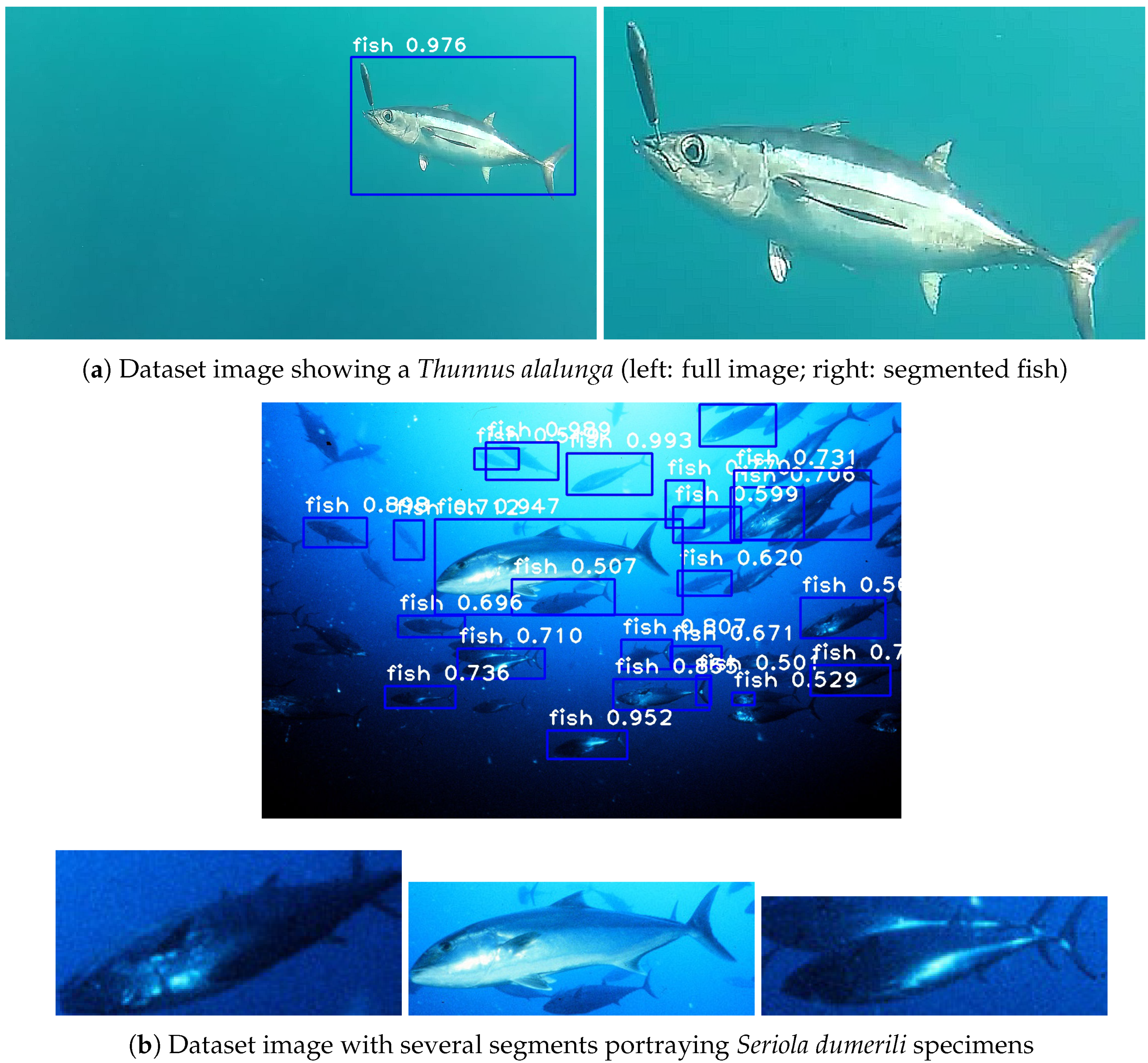
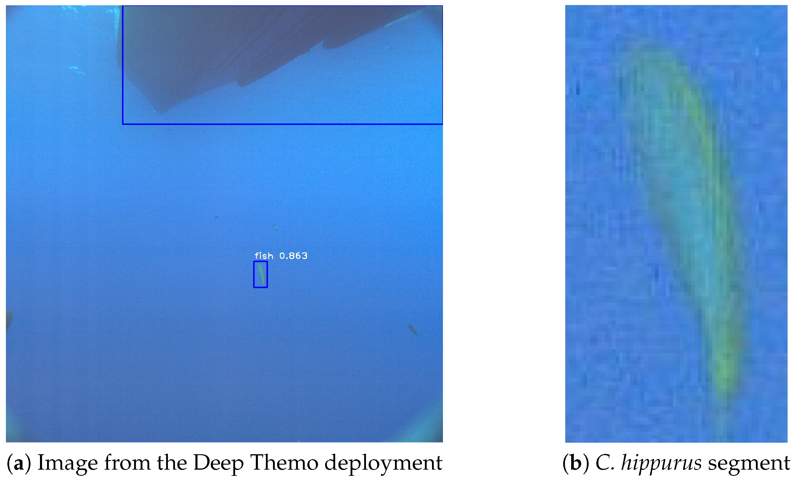
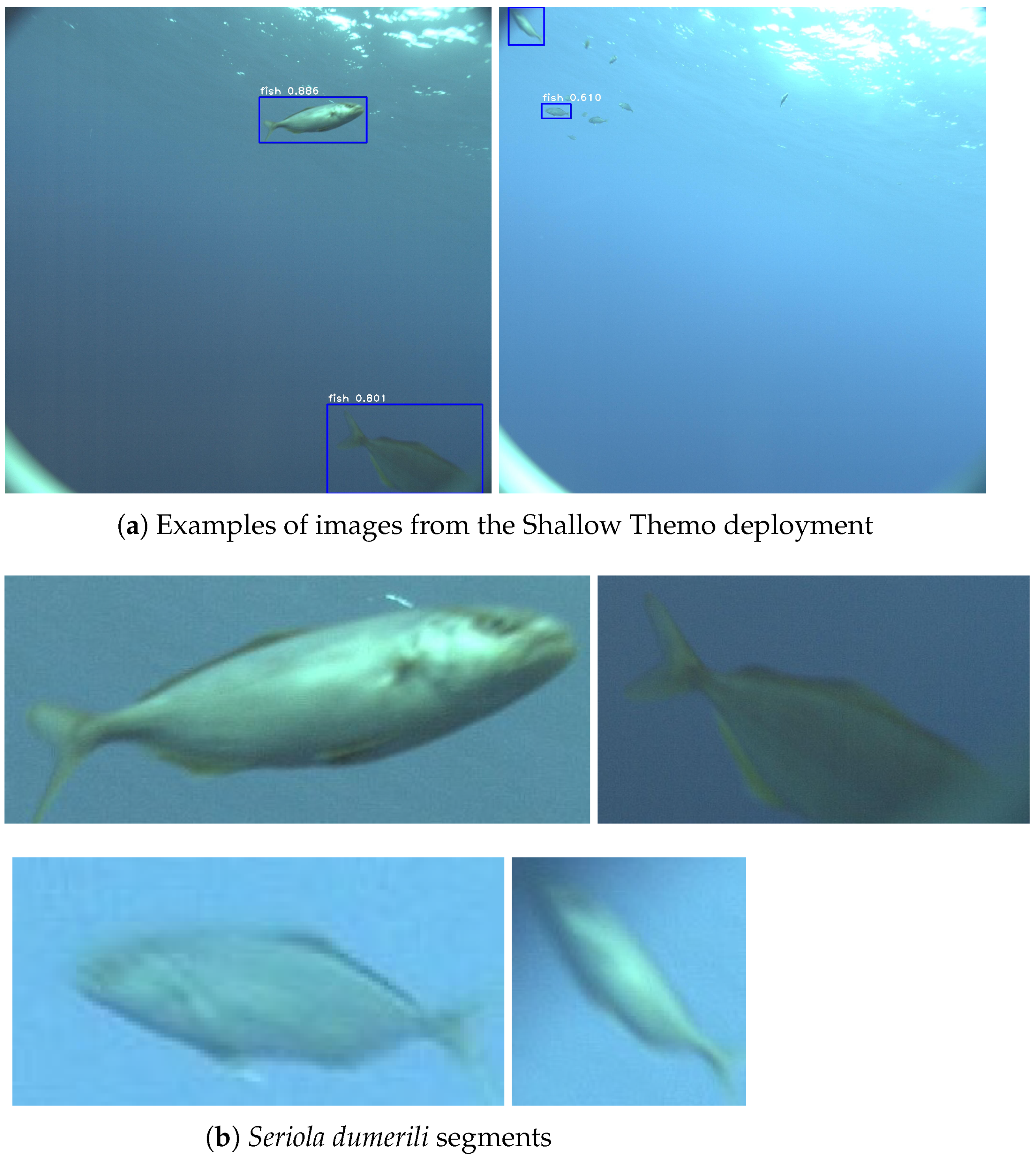
A considerable challenge, in our work, is to produce relevant datasets containing images of Symbiosis’s target pelagic fish species. While many fish image and video repositories exist, most scenes are captured outside the water, and portray additional subjects (e.g., a person fishing) or non-natural backgrounds (e.g., the floor of a sailing ship or fishing boat). We chose to avoid such scenes, as they do not conform to the operational environment of the Symbiosis platform. Hence, we decided to use only observation photos and videos, showing the fish specimens swimming free underwater (see
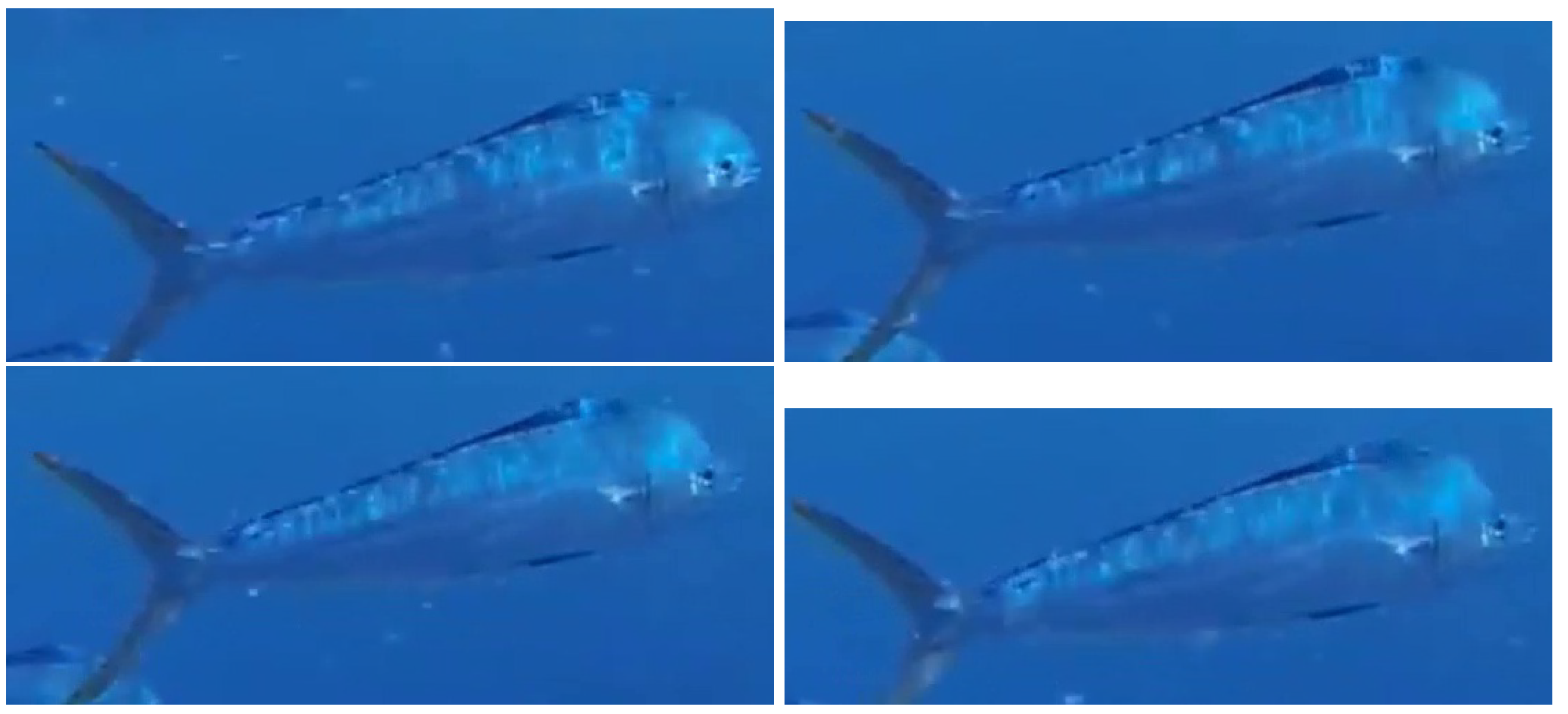
Figure 2). Unfortunately, there exists a limited number of such images and videos, since the target specimens usually live in comparatively deep waters. Multiple fish images can be extracted from each video: the drawback is that these images will typically show a few specimens, possibly grouped together, and repeated across several subsequent frames from the same video (see
Figure 3). These issues make it challenging to train our deep neural networks. In order to mitigate the limited variety in the dataset and the presence of similar individuals, we have proceeded along the following two directions: (1) we have removed very similar fish images, (2) we employ images taken from different videos when setting up the training and test datasets.
1.5. Our Contributions and Main Results
The main contributions of this paper are:
the engineering and evaluation of small neural network models that can be implemented with constrained embedded platforms;
a training method that works with small and unbalanced datasets, often taken from similar images extracted from videos;
a method that assists the decisions of the classifier through object tracking.
With reference to
Figure 1, image processing in the Symbiosis platform has the objective to (i) automatically detect fish in a sequence of video frames and segment them, and (ii) to classify the fish segments and predict the species of the specimens therein. For both problems, we employ convolutional neural networks. The former problem, image detection and segmentation, takes place through a method independently developed, which uses a specifically trained instance of the neural network RetinaNET [
27,
28].
Then, the latter problem, image classification, which is the focus of this paper, exploits different convolutional architectures to identify the segments that contain one of the six pelagic fish species of interest for Symbiosis. The first step to achieve this is to tell apart those segments containing irrelevant fishes or non-fish artefacts (binary classification), which is followed by a second step in which individual fish species are determined (multi-class classification). For comparison purposes, we consider image classification with several popular convolutional architectures, such as VGG16 [
29], François Chollet’s architecture [
30], as well as the more recent RBB [
31] and MobileNetV3 [
32] networks. The latter has been specifically designed with the computation capabilities of mobile devices in mind. With respect to the above works, in this paper we advocate the use of much smaller neural network models, with fewer than 20,000 weights. These models can run in much shorter time than the deep convolutional networks found in popular image recognition models such as RetinaNet [
27] and VGG [
29], and thus require much less energy. This aspect is very relevant for embedded systems that run unattended in the wild. Moreover, we show that tracking objects across multiple images or video frames increases the classification accuracy by up to 7%. We thus advocate this method as a promising alternative for those cases where limited training data may reduce classification accuracy.
A preliminary version of this paper discussing offline training issues was presented at the IEEE/MTS Global OCEANS 2020 Conference [
33].
The structure of the paper is as follows.
Section 2 discusses theoretical aspects, including a brief overview of the neural architectures we employ in this work, the object tracking method, and the components of our data pipeline.
Section 3 presents experimental results both for binary classification and for multi-class classification, including the impact of object tracking on the accuracy of the classification task. In
Section 4 we describe the actual Symbiosis system, and present the results of two sea trials performed with the Symbiosis platform in deep and shallow Eastern Mediterranean Sea waters. Finally,
Section 5 concludes the paper.
2. Theoretical Aspects
The above literature review confirms that, with the exception of a few works, the greatest majority of recent image classification approaches employ a form of convolutional neural networks, either in combination with classical techniques (which carry out feature extraction, denoising, or other preprocessing steps before the convolutional network classifies the input based on extracted features), or in an end-to-end manner (where the convolutional network is designed to directly operate on the input image, extracting relevant features, and complete the classification task). More broadly, deep learning algorithms have replaced hard-coded approaches as a de-facto standard for vision tasks, thanks to their relatively easy domain adaptation and to the limited complexity of the model generation steps.
In our work, we focus on two kinds of benchmarking tasks: (i) binary classification, to tell apart the six species of interest of Symbiosis from other species; and (ii) multi-class classification, to distinguish specimens belonging to each of the six Symbiosis species. To make the most of hardware limitations on embedded platforms, we elect to use small neural architectures with between 10,000 and 20,000 trainable parameters. As shown in
Figure 1, the classification task proceeds through two subsequent steps: image classification (either binary or multi-class) and object tracking. For tracking, we use the SORT [
34] algorithm. We exploit tracking to recognize images that represent the same fish, typically across multiple subsequent frames of a video. These images, once segmented, are classified separately. The output of the classifier is a vector of probabilities for each image, that describes how confidently the classifier predicts the image to pertain to one of seven classes: one class for each the six Symbiosis species, plus one additional class for any
other species not of interest. A voting system then decides on the accepted result, and assigns a final label to each detected object.
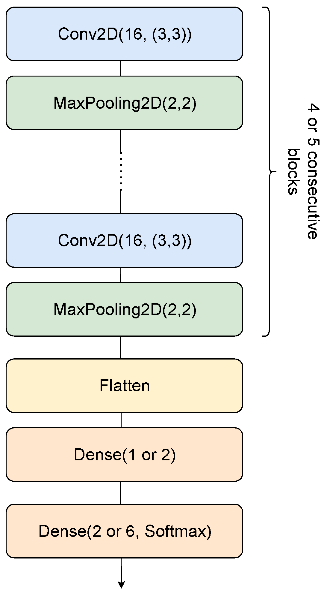
The centerpiece of the pipeline are the proposed small architectures. They are essentially variations on the same structure, as seen in
Figure 4, starting with an alternation of 2D convolutions followed by MaxPooling layers (forming the feature extraction component of the network) and finishing with a set of dense layers (composing the classifier part). In terms of nomenclature, for the scope of readability, we chose to name the networks based on their structure. As such,
refers to 4 initial blocks of 2D convolutions with 16 filters followed by MaxPooling, and a classifier component formed by a dense layer of 8 units, one of 16 units, and a final dense output of
y units, where
y is the number of classes of the particular experiment.
We compare our architectures against well-known networks, namely VGG16 [
29], a baseline convolutional architecture proposed as part of the Keras library tutorial, which we chose to denote as the
Chollet architecture [
30] (after the initiator of Keras), the RBB network [
31], and the MobileNetV3 architecture [
32]. The RBB network consists of two convolutional input layers, followed by 16 residual blocks, an average pooling as well as a 1056-size fully-connected layer. The residual blocks are composed of 3 convolutional layers and a skip-connection. In order to exploit the complexity of the learned representations, RBB increases the number of convolutional filters in the residual blocks, with the network depth. A result of this architecture is the very large number of parameters. The MobileNetV3 networks are bottleneck convolutional networks (i.e., where the size of the representation decreases by proceeding deeper through the network) specifically designed to be applied on mobile devices, under memory and computational constraints. Two similar architectures of different size have been proposed, dubbed “Large” and “Small” in this paper. A detailed description of the networks is provided in [
32] (Tables 1 and 2). The RBB and MobileNetV3 networks have been specifically proposed for mobile deployments in the literature.
All architectures discussed in the present paper are listed, together with their number of trainable parameters, in
Table 1. The proposed architectures have between 10 and 20,000 parameters, with one exception of roughly 50,000 parameters. In all cases these numbers are considerably smaller than the 1.6 million parameters of Chollet, the 3 to 8.7 million parameters of MobileNetV3, the over 15 million parameters of VGG16, and the almost 70 million of RBB. In particular, we observe that the RBB network is three orders of magnitude larger than the networks we propose, and hence will not be considered as a practical option. The MobileNetV3 networks also have two orders of magnitude more parameters than our networks.
3. Experimental Results
3.1. Image Dataset Creation
Neural networks require a large set of training examples. This is especially true for the deep architectures employed for image processing and recognition. In the absence of a sufficiently rich dataset, the many trainable parameters (or weights) of the network converge to values that overfit the limited number of training examples provided, so that the model becomes unable to generalize to different, previously unseen images [
35]. Moreover, for classification problems, the training set should representing the different classes uniformly, so that the neural network does not “specialize” on a specific class while remaining unable to recognize the others. In Symbiosis, one of the most challenging tasks was precisely to compile a reasonably large and curated training dataset. This required us to collect, clean and aggregate a sufficiently large quantity of images in a homogeneous form, along with their corresponding relevant meta-data: labels, bounding boxes (regions of interest, or ROI), etc.
Symbiosis focuses on the recognition of images portraying one of six species of bony fishes (see
Figure 5), selected based on their commercial value, their behavior (e.g., schooling or not schooling), appearance, as well as occurrence at the foreseen deployment locations in the Eastern Mediterranean Sea and in the Red Sea. These species of interest are:
Albacore tuna (Thunnus alalunga).
Greater amberjack (Seriola dumerili).
Atlantic mackerel (Scomber scombrus).
Dorado (dolphinfish, Coryphaena hippurus).
Mediterranean horse mackerel (Trachurus mediterraneus).
Swordfish (Xiphias gladius).
The Biology team of the Symbiosis project helped compile a first dataset containing raw data from multitude of private and public data sources. This included underwater videos and photographs of the above six species. Each item was manually revised and labeled as one of the six species, and those images and videos that included several different species were discarded in this phase to help dataset labeling. After extracting frames from the videos, we formed a first collection of training samples by segmenting the extracted frames and images through the algorithm in [
28]. This produced about 1.5 million image segments, each containing a region-of-interest (ROI) with a potential fish. As the algorithm was still being optimized at the time, we proceeded by inspecting all images manually to discard those that did not contain a fish, or those where the size or quality of the fish image was too low, leaning itself to misinterpretation even by a human. This filtering process was based on such fish body features as minimum size, as well as image quality features such as full or partial fish body coverage, general image quality, and the detection accuracy reported by the algorithm in [
28]. Initially, we crowdsourced part of the process. However, the majority of the image quality assurance and validation process was completed manually by the Symbiosis team, and yielded 51,260 validated segments. It is worth mentioning that some of the segments included in the data set would not allow a human expert to identify the species. They have been maintained in the hope that the neural networks are able to extract and use features that humans cannot, especially when an object tracking process presents a sequence of images of the same object to the classification algorithm.
We employed the Symbiosis dataset for both classification tasks of interest in this work: binary classification (meaning that the algorithm should distinguish between our species of interest, grouped into two classes), and multi-species classification (or distinguishing among our six species of interest). For this purpose, we split the dataset into train, validation and test subsets, containing a distribution of (60%, 20%, 20%) of the dataset related to each species. It is worth noting that we kept segments from the same videos together in the same set during this process. This data organization further helps limit overfitting by avoiding that very similar images from the same video spread from the training set to the validation and test sets. The size of the Symbiosis dataset for each of the six Symbiosis species appears in
Table 2. We observe that the total number of images is not exceedingly small, yet these images are very unevenly distributed among the six species, reaching a maximum coverage of
Seriola dumerili with about 14,300 images, and a minimum coverage of
Trachurus mediterraneus, with about 3200 images.
3.2. Classification Process
As mentioned above (see also
Figure 1), our optical detection and classification process consists of two separate stages that rely on convolutional neural networks: (1) detection and segmentation, that relies on a retrained version of RetinaNET [
27] to identify areas corresponding to fish images in a raw image or video frame [
28]; and (2) classification, where each segment is processed to determine if it portrays one of the six species of interest, and which one. In this paper, we focus on the engineering of light architectures with the aim to provide results comparable to well-known networks (such as VGG16 [
29] or the Chollet architecture [
30]).
We recall that all architectures we engineer in this paper have a similar structure, namely a sequence of pairs of layers, where each pair contains a convolutional layer followed by a max pooling layer (denoted
and
M, respectively). After these pairs, comes a sequence of dense layers (denoted
,
), and a final classification layer (
,
, see
Figure 4). We remark that we leverage the pre-trained version of VGG16, and rather only re-train the final layer of the architecture using our particular dataset.
When images are segmented from subsequent video frames, tracking becomes an option to help the classification task. Our tracking component exploits SORT, an open-source tracking algorithm that performs well in the presence of typical fish mobility [
36,
37,
38]. We did not build a third deep learning model for this purpose, in order to keep the computational complexity low, and thus facilitate the deployment of the algorithm on constrained embedded systems. The tracker receives image segment coordinates from every subsequent frame, that correspond to two opposite corners of each ROI. It then provides an artefact identifier and the predicted position of the object, in the next frame. We then compare the predicted coordinates with the actual coordinates of the artifact in a subsequent frame by computing the ratio between the intersection and the union of two segments, i.e., the intersection over union (IoU) metric. For those segment pairs where the metric is maximum and exceeds a predefined threshold, we declare the artifacts to represent the same subject across subsequent frames. It is worth mentioning that the tracker updates its predictions on a per-frame basis, even when the tracked object is missing in some frame. This is particularly useful if the detection and segmentation stage outputs a false negative in an intermediate frame, something that is likely to happen in videos with a low frame rate.
3.3. Classification Results with and without Tracking
To evaluate our neural network architectures, we have produced two versions of the Symbiosis dataset: in the first version, we group the six species of interest into two classes, one including all instances of
Seriola dumerili and
Coryphaena hippurus, and another class grouping the remaining species; in the second version, we keep the classes separate, such that each class represents a different species. We then employ the first dataset for binary classification, and the second for multi-class classification, respectively. We remark that the above binary classification experiment is slightly different from the focus of Symbiosis, which would require us to differentiate between the species of interest for Symbiosis and all other species. However, performing the above experiment allows us to (i) rely on a sufficiently balanced dataset; (ii) train and test our networks using data taken in a uniform environment; (iii) employ images validated by experts; and (iv) evaluate the impact of tracking on the quality of the classification. Later on, in
Section 3.4, we will instead comment on the results of a proper binary classification experiment, that distinguishes Symbiosis species from other species depicted in independently collected photo datasets.
The setup for our experiments is identical in both cases: segmented images are first sent to a classifier, in order to establish the fish species. A group of segmented images, along with their class, are combined via tracking, in order to determine if the segments represent the same object. In the presence of a positive tracking output, that ties multiple images to the same subject, we place classification results into a vector, and use one of three methods to finally identify the fish species: by taking the mean of all values (denoted as Mean), by taking the maximum value (Max) or by using a majority voting scheme (Voting). We then employ the final classification result to compute the accuracy of our algorithm.
We present the results of binary classification in
Table 3. We observe that the VGG16 architecture achieves the best accuracy (about 74%) without tracking. However, this comes at the cost of a complex deep neural network, having more than 15 million parameters, and requiring significant computational power on embedded devices. Conversely, our
architecture achieves 62% accuracy with fewer than 11,000 parameters. A second observation from
Table 3 is that tracking increases the accuracy, in some cases significantly (about 8% for Chollet and up to 4% for our architectures).
Table 4 provides the results of multi-class classification among the six Symbiosis species. Here, VGG16 achieves again the highest accuracy (more that 51% without tracking and almost 56% with tracking), but our much simpler architectures with roughly 14,000 parameters have also a workable accuracy of more than 39% without tracking, and more than 44% with tracking. Like for binary classification, tracking significantly improves accuracy.
In order to compare these results with state-of-the-art mobile networks, we have run the multiclass classification with the MobileNetV3 networks [
32]. Interestingly, even with the large number of trainable parameters of these networks, the average accuracy obtained is roughly 25% (
% with MobileNetV3 Large and
% with MobileNetV3 Small). This is much lower than the accuracy obtained with the other networks.
It is important to point out that the VGG16 has been pre-trained, and can thus take advantage of previously-learned parameters. Furthermore, relatively small datasets can prevent large architectures from achieving their peak representational capacity, due to overfitting (potentially explaining the relatively poor performance of architectures such as Chollet). In practical applications, data collected from probes such as the one used in the present experiments is typically scarce. As such, small architectures benefit from fast adaptability to small datasets, apart from their very low computational requirements.
3.4. Additional Image Classification Results
We present now additional classification experiments performed with the different architectures presented. These experiments include binary classifications that are similar to the one of the the Symbiosis system, since they classify between the six target fish species and other species. In these experiments the data available does not allow the use of tracking, since the new dataset used does not contain videos, and they only evaluate the performance of the classification process of individual images. The datasets used in these experiments are the following.
Symbiosis-NCC dataset: This dataset contains a subset of the segments in the Symbiosis dataset, in which images are guaranteed to have Normalized Cross-Correlation (NCC) below 50%. The NCC filter applied to the original Symbiosis dataset removes segments of the same fish extracted from the same video that are very similar. The number of images of each species in the Symbiosis-NCC dataset are shown in
Table 5. The total number of images is 9262, all of our 6 species of interest.
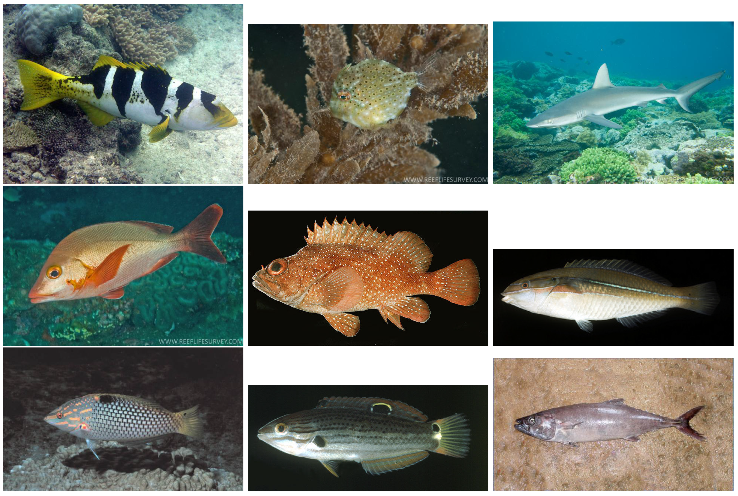
QUT+NOA dataset: 4372 images of QUT
2 (see also
Figure 6) and 749 images of NOAA
3, totaling 5121 images. These are collections of fish images, which do not include videos. They include mostly reef fishes, and do not include images of our 6 species of interest.
Table 5.
Number of images per species in the Symbiosis-NCC dataset, obtained from the Symbiosis dataset after filtering in order to have Normalized Cross-Correlation below 50%.
Table 5.
Number of images per species in the Symbiosis-NCC dataset, obtained from the Symbiosis dataset after filtering in order to have Normalized Cross-Correlation below 50%.
| Species | Number |
|---|
| Thunnus alalunga | 768 |
| Seriola dumerili | 1832 |
| Scomber scombrus | 1575 |
| Coryphaena hippurus | 3398 |
| Trachurus mediterraneus | 628 |
| Xiphias gladius | 1061 |
| Total | 9262 |
With these datasets we have carried out 3 experiments, two of binary classification and one of multi-class classification.
Binary–No mix: In the first binary experiment the two classes are the images from the Symbiosis-NCC and QUT+NOA datasets, respectively. These images are split among training, validation, and test sets in a proportion of roughly (80%, 10%, 10%), but making sure that images from the same video in the Symbiosis dataset are all in one set (see
Table 6).
Binary–Mix: In this second binary experiment, the split strategy of the QUT+NOA dataset is the same used in the first one, while the Symbiosis-NCC is split randomly in exactly (80%, 10%, 10%) proportions. This means that images from the same video may be in the training and test sets. This may help increase the accuracy since these images may be similar (although their NCC is below 50%).
Multi-class–Mix: In the multi-class classification experiment the Symbiosis-NCC dataset is randomly split in exactly (80%, 10%, 10%) proportions, as shown in
Table 7. Again, images form the same video can fall in different sets.
Table 6.
Split of the datasets used for the
Binary–No mix classification of
Table 8. In the Symbiosis-NCC dataset, segments from the same video are in the same set (among train, validation and test).
Table 6.
Split of the datasets used for the
Binary–No mix classification of
Table 8. In the Symbiosis-NCC dataset, segments from the same video are in the same set (among train, validation and test).
| Dataset | Train | Validation | Test | Total |
|---|
| Symbiosis-NCC | 7863 | 676 | 723 | 9262 |
| QUT+NOA | 4097 | 512 | 512 | 5121 |
Table 7.
Split of the Symbiosis-NCC dataset used for the
Multi-class–Mix classification of
Table 8. Segments from the same video could be placed in several sets of train, validation and test.
Table 7.
Split of the Symbiosis-NCC dataset used for the
Multi-class–Mix classification of
Table 8. Segments from the same video could be placed in several sets of train, validation and test.
| Species | Train | Validation | Test | Total |
|---|
| Thunnus alalunga | 614 | 77 | 77 | 768 |
| Seriola dumerili | 1464 | 184 | 184 | 1832 |
| Scomber scombrus | 1260 | 158 | 158 | 1576 |
| Coryphaena hippurus | 2718 | 340 | 340 | 3398 |
| Trachurus mediterraneus | 502 | 63 | 63 | 628 |
| Xiphias gladius | 840 | 106 | 106 | 1052 |
Table 8 shows the accuracy of the 3 experiments. All experiments have large accuracy. As can be seen, the
Binary–Mix experiment has slightly higher accuracy than that of
Binary–No mix, which seems to indicate that training and testing with images from the same video indeed helps. This is also confirmed by the fact that accuracy of the experiment
Multi-class–Mix is much higher than the one observed in the previous section,
Table 4. One important remark that must be made here is that, while training and testing with images extracted from the same video may indeed be helpful to increase the accuracy of the models, care must be taken that the frames representing different examples are sufficiently different to prevent simple memorization.
In this work we applied a filter that provided an indication of the level of similarity between two frames, and discarded the ones that were not sufficiently distinguishable. Furthermore there is a risk that the model may learn other background objects that may appear in two images, and use them in the classification process. This problem is partially mitigated by the similarity filter and partially by the object detection and cropping performed prior to classification, a process that removes most of the surrounding background.
It is worth mentioning that the accuracy observed with VGG and Chollet is not significantly higher than the one observed with the small architectures that are proposed in this paper. Yet, all experiments show significantly larger accuracy than those in
Table 3. We believe that this is is due to the different setting of the QUT+NOA dataset, as well as to its limited size (about 1/2 of our dataset). Such differences may lead larger networks such as Chollet and VGG-16 to overfit the classification problem, including the chance that classification relies not just on the morphological characteristics of the fish, but also on other image features, including the background. Conversely, our smaller networks have a more limited data representation power, and are less prone to overfitting.
Table 8.
Accuracy of the additional experiments:
Binary–No mix is a binary classification experiment using the dataset QUT+NOA versus the Symbiosis-NCC dataset of
Table 5, with the split of
Table 6.
Binary–Mix is a binary classification experiment using the dataset QUT+NOA versus the Symbiosis-NCC dataset of
Table 5, with a (80%, 10%, 10%) split.
Multi-class–Mix is a multiclass classification experiment using the Symbiosis-NCC dataset of
Table 5, with the (80%, 10%, 10%) split of
Table 7.
| Architecture | Binary | Binary | Multi-Class |
|---|
| No Mix | Mix | Mix |
|---|
| | | |
| | | |
| | | |
| | | |
| | | |
| VGG16 | | | |
| Chollet | | | |
5. Conclusions
Underwater fish recognition via autonomous probes that rely on constrained embedded computers is a challenging tasks, due to limitations on computational power, memory availability, and image quality, among others. Considering the above constraints, in this work we engineered convolutional neural network models to yield architectures of limited complexity and much fewer trainable parameters than complex object recognition architectures such as VGG16 or MobileNet. We showed that our solutions produce results comparable to such much larger and broadly used architectures, especially when aided by a computationally inexpensive object tracking algorithm that combines multiple classified images to yield a more accurate output.
Our experience in this work suggests that the most challenging task is the acquisition and preparation of a dataset. In general, the number of relevant images available for the classes of interest is limited, especially considering that the images should be captured under water. We compensated for the lack of images by extracting relevant segments from video frames, and mitigated the higher dataset similarity that results by placing nearly identical images only in one subset among training, validation, and test.
The imbalance of the training data also posed a significant challenge. As seen in
Table 2, the number of images collected for the different species of interest in our work is very different. We argue that this is one possible reason causing a lower classification accuracy in our models: for binary classification, where the six classes have been split into two categories by maintaining a similar number of images per class, some of our architectures yield comparable results with respect to VGG16, which has two orders of magnitude more parameters. Future work includes collecting more images to balance the dataset, as this will result in a performance improvement for our models.


 ,
, 
