Back Projection Algorithm for Multi-Receiver Synthetic Aperture Sonar Based on Two Interpolators

Abstract

The back projection (BP) algorithm is characterized by its high performance for multi-receiver synthetic aperture sonar (SAS). For this reason, it is usually used to evaluate the imaging performance of Fourier-domain methods. However, this algorithm suffers from a large computation load, and the imaging efficiency is seriously lowered. In order to improve the imaging performance, this paper proposes focusing the multi-receiver SAS data using the BP algorithm based on two interpolators, including the linear interpolation and nearest-neighbor interpolation. The former interpolation is used to decrease the interpolation error based on adjacent sampled data; the latter estimates the data at the desired moment by assigning the data value of the nearest sample as estimated data. Then, the imaging performance of the presented method is discussed in detail based on simulations and real-data processing. With the presented method, the imaging performance can be improved without a loss of efficiency compared to nearest-neighbor interpolation without an upsampling operation. In comparison with the traditional BP algorithm, the presented method can be used to improve the imaging efficiency without any loss of performance.

1. Introduction

Synthetic aperture sonar (SAS) [1,2,3] is a high-resolution technique used in the underwater field. The SAS technique is mostly the same as its counterpart, synthetic aperture radar (SAR) [4,5,6,7,8,9,10,11,12,13]. For SAS systems, synthetic aperture image formation is an important issue. Figure 1 depicts the system model of synthetic aperture sampling and SAS focusing. For SAS echo sampling, the input is target formations such as complex reflectivity. During sonar movement in the along-track dimension, the pulsed sonar continuously transmits a wideband signal and receives an echo signal reflected by the target. This echo signal is considered the output of the SAS echo sampling system. In fact, target information such as complex reflectivity, relative range, and the bearing angle between target and sonar is also collected by the received echo signal. From Figure 1, it can be seen that SAS focusing is just the inverse process of the echo sampling system. By designing the system transfer function, the objective of any focusing algorithm is to invert the SAS sampling in order to provide a map of target reflectivity. At this point, the SAS system can form an image of the complex reflectivity of an area by coherently combining successive echo signals that are transmitted, reflected by various targets, and received by the system. Since the virtual synthetic aperture array is formed, SAS focusing makes it possible to achieve an along-track resolution that is independent of range and signal frequency, and that is only determined by the width of the real aperture. Consequently, target recognition, target detection, shipwreck salvage, underwater archaeology, underwater remote sensing, and so on can be easily carried out with high-resolution SAS images. Imaging algorithms including Fourier-domain algorithms and time-domain algorithms are being investigated by researchers all over the world.

The multi-receiver SAS system includes double square-rooted terms [14,15,16]. It is difficult to deduce the system transform function in the two-dimensional (2D) frequency domain, as the stationary point cannot be analytically calculated based on the stationary phase method. Therefore, users often adopt some indispensable approximations in order to exploit frequency-domain algorithms. Monostatic-SAS-based methods [17,18,19,20] firstly convert the multi-receiver SAS data into a monostatic-SAS signal by compensating some approximation errors with the preprocessing step. Then, traditional Fourier-domain algorithms can be directly applied. Generally speaking, it is difficult to completely compensate the approximation errors [18], which are spatial variants. Many other methods, such as the Lagrange inversion theorem [21], the series reversion method [22,23,24], and the equivalent transformation of radical expression [25], are used to analytically deduce the stationary phase point and the system transform function in the 2D frequency domain. Based on the Lagrange inversion theorem, the stationary phase point is approximated via series expansion. With the series reversion method, both the double square-rooted terms and the stationary phase point are approximated via series expansion. Through the equivalent transformation of radical expression, the double square-rooted terms are approximated using a single square-rooted term. We find that these methods still suffer from approximation errors, which can degrade the imaging performance. To avoid this approximation, the numerical method [26,27] is used to deduce the stationary phase point and system transform function. To some degree, the system transform function can be considered accurate; however, the space variance of this function makes it challenging to develop fast imaging algorithms. To handle this issue, the range sub-block is often exploited. However, this operation can lead to further errors for the targets not located within the reference range.

The BP algorithm [28,29,30], characterized by its high performance, is often considered to be the most precise method, as the system transform function does not use any approximations. The approximation only lies in engineering applications such as interpolation. The results are usually used as the criteria to evaluate the imaging performance of fast Fourier-domain methods, since the essence of fast methods is to approximate the system transfer function of the BP algorithm based on some approximations. Based on the linear time invariant system in the signal processing field [31], the system transfer function is a link between the input and output. Therefore, the system transfer function needs to be obtained before synthetic aperture imagery. The BP algorithm can also be easily integrated with the motion compensation algorithm in comparison with fast algorithms. However, this method is time-consuming, and it cannot satisfy the demand of real-time processing required by current SAS systems. In general, there are two methods to improve the efficiency. One is to optimize the BP algorithm based on software, and the other is to adopt more high-performance hardware. In [32], fast Fourier transformation (FFT) is used by the BP algorithm. Unfortunately, the efficiency is improved slightly. The fast-factorized BP (FFBP) algorithm [33,34,35,36] is further presented to improve the efficiency. The basic idea of this method is to factorize into many stages. The full synthetic aperture is divided into many sub-apertures, and then the coarse sub-images are obtained by back-projecting the sub-aperture data into the sub-image grid. The final image is formed by recursively combining these coarse sub-images. However, this method suffers from a balance between accuracy and efficiency. That is to say, the efficiency is obtained at the cost of accuracy. The efficiency can be further improved using high-performance hardware such as graphics processing units (GPU) [37,38,39], NVIDIA compute unified device architecture (CUDA) [40], field-programmable gate array (FPGA) [41], and so on. In practice, the computation load of the BP algorithm is not lowered, and the imaging efficiency highly depends on the hardware. When users want to obtain real-time processing results, the expensive hardware must be purchased.

To improve the imaging efficiency of the BP algorithm without loss of accuracy and expensive costs, this paper presents a new BP algorithm for the multi-receiver SAS system based on two interpolators, including linear interpolation and nearest-neighbor interpolation. The presented method firstly reduces the interpolation error by using linear interpolation, and then estimates the data at the desired moment by assigning the data value of the nearest sample as estimated data with the nearest-neighbor interpolation. Based on this method, the imaging efficiency can be improved significantly compared to the traditional BP algorithm. With the presented method, the imaging performance can be improved without any loss of efficiency compared to nearest-neighbor interpolation that does not have an upsampling operation. The paper is organized as follows. Section 2 presents the signal model. Section 3 describes the presented method. In Section 4, some simulations discussing the influence of sampling rate on the imaging performance are analyzed in detail. Finally, the conclusions are presented in the last section.

2. Multi-Receiver SAS Signal Model

In this section, we discuss the multi-receiver SAS signal model. The 2D imaging geometry is shown in Figure 2. The sonar moving direction is denoted as the along-track dimension. The cross-track dimension is the slant range. The sonar carrier velocity is denoted by v, and the sound speed in water is c. The black rectangle depicted in Figure 2 represents the transmitter. The remaining rectangles denote the receivers. These receivers are combined to form a receiver array, which is aligned in the along-track dimension. We suppose that there are total M receivers. The distance between the transmitter and the m-th receiver is d_m. The subscript m ($m\in [1,M]$) is the receiver index. The slow and fast times corresponding to the along-track and cross-track dimensions are t and $\tau$, respectively. For simplicity, we suppose that there is an ideal point target in the imaging scenario. In Figure 2, the red star stands for the ideal point target. The coordinate in the cross-track dimension is r and in the along-track dimension is x_n.

When the transmitter moves to the position vt in the along-track dimension, the chirp signal is broadcast by the transmitter. The path between the transmitter and target is $R_T\left(t\right)=\sqrt{r^2+{\left(vt\right)}^2}$. During the signal transmission, the receiver array is continuously moving forward in the along-track dimension. The moving distance is $v\cdot {\tau }_m$. Here, the accurate time delay of the echo signal received by the m-th receiver is given by:

$$\begin{array}{l}{\tau }_m=\frac{v\left[(vt-x_n)+d_m\right]+c\sqrt{{(vt-x_n)}^2+r^2}}{c^2-v^2}+\\ \frac{\sqrt{{\left\{v\left[(vt-x_n)+d_m\right]+c\sqrt{{(vt-x_n)}^2+r^2}\right\}}^2+(c^2-v^2)\left[2(vt-x_n)d_m+d_m{}^2\right]}}{c^2-v^2}\end{array}$$

(1)

For the traditional SAS system, the sonar transmits and receives the signal when the sonar is located at an along-track position $v\cdot {\tau }_m$. In practice, the receiver continuously moves in the along-track dimension. Before receiving the echo signal, the along-track forward distance of the i-th receiver is $v\cdot {\tau }_m$. Traditional SAS neglects the receiver-forward distance during the signal propagation. This would lead to image distortion when the SAS system works with a fast mapping rate [23]. Fortunately, Equation (1) considers the forward distance during the signal propagation. It can be deduced based on the geometry triangle formed by the transmitter, receiver, and target in Figure 2. A detailed deduction can be found in [19]. Then, we can obtain the distance $R_{Rm}\left(t\right)=\sqrt{r^2+{(vt+d_m+v\cdot {\tau }_m)}^2}$ between the target and the m-th receiver. Therefore, the two-way slant range is expressed as

$$R_m\left(t;r\right)=R_T(t)+R_{Rm}(t)=\sqrt{r^2+{\left(vt\right)}^2}+\sqrt{r^2+{(vt+d_m+v\cdot {\tau }_m)}^2}$$

(2)

After signal demodulation, the echo signal of the m-th receiver is written as

$$s{s}_m(\tau ,t)=p\left(\tau -\frac{R_m\left(t;r\right)}{c}\right){\omega }_a(t)\cdot \exp \left\{-\mathrm{j}2\mathsf{\pi }{f}_c\frac{R_m\left(t;r\right)}{c}\right\}$$

(3)

In Equation (3), $p\left(\tau \right)$ is the transmitted signal. ${\omega }_a(t)$ is the composite beam pattern denoted by the transmitter and receiver. As the SAS imagery lies in the coherent phase processing, we neglect the influence of ${\omega }_a(t)$ in the following discussion. $f_c$ is the center frequency.

3. BP Algorithm

This section discusses the presented BP algorithm based on nearest-neighbor interpolation.

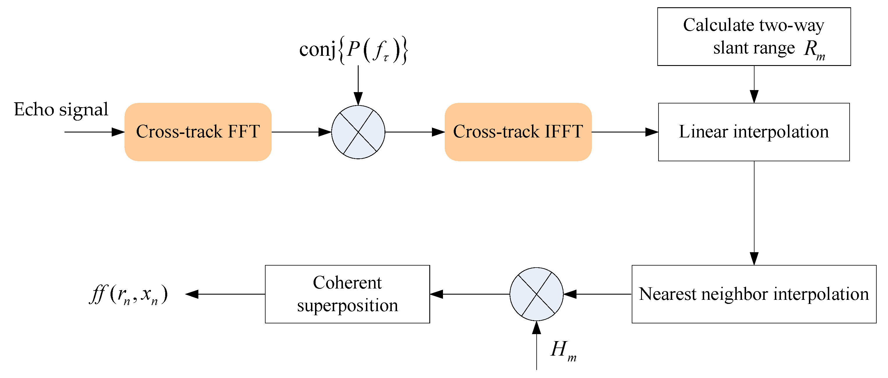
3.1. Presented Method

The basic idea of the BP algorithm is shown in Figure 3. Figure 3a shows an arbitrary target in the object space, and its coordinates are $(r_n,x_n)$. The curve in Figure 3b denotes the range compressed signal corresponding to each received position. In Figure 3b, all curves in the along-track dimension are aligned in the red line, which is called the range migration path. It is caused by the relative distance denoted by Equation (2) between the sonar platform and the target. After superposing the echoes back-projected into the image space along the range migration path, the complex image shown in Figure 3c can be obtained.

The first step is to compress the echo in the cross-track dimension. This operation can be conducted in the frequency domain based on the matched filtering. This processing is given by

$$S{s}_{cm}(f_{\tau },t)=S{s}_m(f_{\tau },t)\cdot \mathrm{conj}\left\{P\left(f_{\tau }\right)\right\}$$

(4)

In Equation (4), $f_{\tau }$ is the instantaneous frequency in the cross-track dimension. $S{s}_i(f_{\tau },t)$ is the spectrum after performing FFT in the cross-track dimension with respect to (3). $P\left(f_{\tau }\right)$ is the spectrum of the transmitted signal. $\mathrm{conj}\{\cdot \}$ denotes the conjugation of transmitted signal. $S{s}_{ci}(f_{\tau },t)$ stands for the compressed signal.

After inverse FFT(IFFT) in the along-track dimension, the signal shown in Equation (4) is transformed into the fast time-domain. The coherent superposition along the range migration path denoted by the red line in Figure 3b is expressed as

$$ff(r_n,x_n)={\displaystyle {\int }_{-0.5x_0}^{0.5x_0}S{s}_{cm}(\frac{R_m}{c},t)\exp \left\{\mathrm{j}2\pi f_c\frac{R_m}{c}\right\}dx}$$

(5)

Here, $x_0$ denotes the synthetic aperture length. In practice, the superposition expressed by Equation (5) cannot be efficiently carried out in the signal processors. The direct scheme is to transform this curve into a straight line. Hereafter, the coherent processing can be directly performed in the along-track dimension. However, the conversion from curve to straight line cannot be simply shifted in the cross-track dimension, as the location of the red line in Figure 3b is not an integral number of the cross-track bin. Therefore, interpolation is usually needed to solve this problem. Traditional interpolators such as sinc interpolators, FFT-based interpolators, and spline-based interpolators are very time-consuming. In order to improve the efficiency, a simple interpolator named nearest-neighbor interpolation is exploited in this paper. In order to accurately use the nearest neighbor interpolation, the data are firstly upsampled using the linear interpolation shown in Figure 4. In Figure 4, the black circles are sampled data, which are $y_0$ and $y_1$ corresponding to knot points $x_0$ and $x_1$, respectively. The basic idea of linear interpolation is to estimate the value at desired point $x$ using adjacent sampled data. From Figure 4, we can obtain the value $y$ along the straight line corresponding to the knot point $x$ ($x_0<x<x_1$), and the expression is given by

$$\frac{y-y_0}{x-x_0}=\frac{y_1-y_0}{x_1-x_0}$$

(6)

Since the knot point $x$ ($x_0<x<x_1$) is given, solving Equation (6) yields the estimated value $y$ expressed as

$$y=y_0+\left(x-x_0\right)\frac{y_1-y_0}{x_1-x_0}=y_0+\frac{\left(x-x_0\right)y_1-\left(x-x_0\right)y_0}{x_1-x_0}$$

(7)

We suppose that the data at two knot points $x_0$ and $x_1$ ($x_0<x_1$) is $q(x_0)=y_0$ and $q(x_1)=y_1$, respectively. Within the interval [x₀, x₁], the value at desired knot point x ($x_0<x<x_1$) is given by

$$q(x)=\{\begin{array}{ll}{y}_1,& 0.5\left(x_1-x_0\right)<x\le x_1\\ y_0,& x_0<x\le 0.5\left(x_1-x_0\right)\end{array}$$

(8)

The interpolation denoted by Equation (8) estimates the data $q(x)$ at the desired moment x by assigning the data value of the nearest sample as estimated data.

After interpolation, compensation of the Doppler phase is carried out, and this operation is expressed as

$$H_m=\exp \left\{\mathrm{j}2\pi f_c\frac{\Delta R_m}{c}\right\}$$

(9)

with

$$\Delta R_m=R_m-2r,$$

(10)

Based on the processing steps described above, a diagram of the presented method is depicted in Figure 5.

3.2. Computation Load

In this section, we discuss the computation load of the presented method. Here, the number of floating point operations (FLOPs) [31] is calculated. We suppose that the SAS data have N_a and N_r sampling points in the along-track and cross-track dimensions, respectively. The image space is also supposed to have N_a and N_r pixels in the along-track and cross-track dimensions, respectively. For SAS imaging algorithms, FFT/IFFT, multiplication and interpolation are mainly exploited. The total number of basic operations is presented in

Table 1. Basic operations used by presented method.

	FFT/IFFT	Multiplication	Linear Interpolation
FLOPs	$5N_{\mathrm{r}}{\log }_2{N}_{\mathrm{r}}$	6	6
Total number	$2N_a$	$N_a{N}_r+N_a^2{N}_r$	$\beta N_a(N_r-1)$
Total FLOPs	$10N_a{N}_r{\log }_2{N}_r$	$6N_a{N}_r+6N_a^2{N}_r$	$6\beta N_a(N_r-1)$

. In Table 1, $\beta$ is the upsampling rate, which means that $\beta$ points between adjacent sampling points are estimated. The computation load of FFT/IFFT for N_r sampling points is $5N_{\mathrm{r}}{\log }_2{N}_{\mathrm{r}}$. The computation load of complex multiplication needs six FLOPs. The linear interpolation shown as Equation (7) can be considered complex multiplication. The nearest-neighbor interpolation does not generate new data. Therefore, the computation load can be neglected. Based on Table 1, we can obtain the total FLOPs, which are given by

$$L=10N_a{N}_r{\log }_2{N}_r+6N_a{N}_r+6N_a^2{N}_r+6\beta N_a(N_r-1),$$

(11)

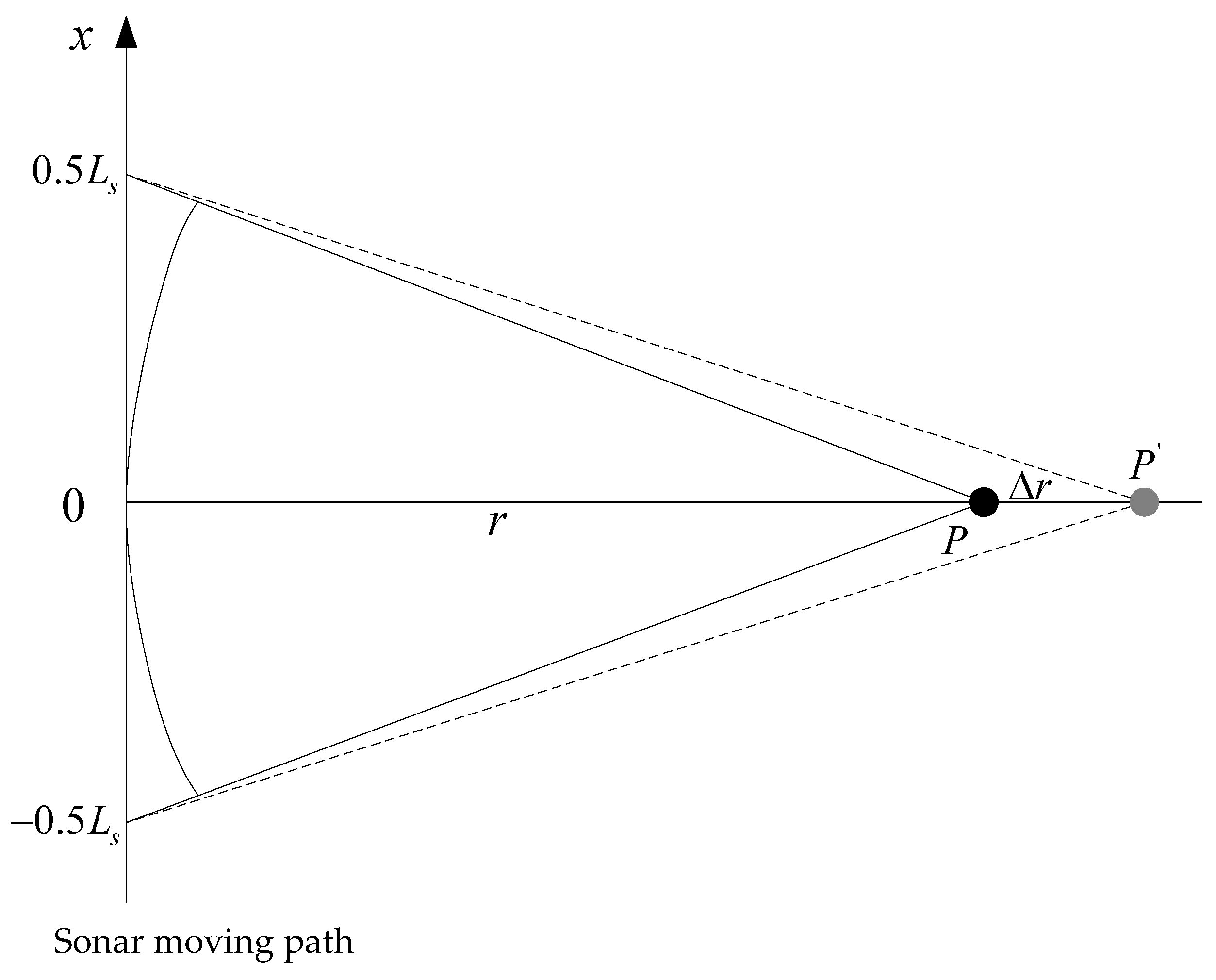
3.3. Discussion of Upsampling Rate

We suppose that there is a point target marked by P in the imaging area. The closest range between sonar and target is $r$. The sonar moves within the synthetic aperture length $L_s$, where the sonar can receive the echo signal reflected by the point target. The wavefront of the received echo signal is a spherical wave, as shown in Figure 6. It can be seen from Figure 6 that the maximum magnitude of the phase error is at the synthetic aperture edge, where the maximum range error is given by

$$\Delta =\sqrt{r^2+{\left(\frac{L_s}{2}\right)}^2}-r\approx \frac{L_s^2}{8r},$$

(12)

Then, the maximum magnitude of phase error is written as

$$\frac{4\pi \Delta }{\lambda }=\frac{\pi L_s^2}{2\lambda r},$$

(13)

where $\lambda$ is the wavelength corresponding to the center frequency $f_c$.

Based on the SAS theory [42], the along-track resolution can be denoted by:

$${\rho }_a=\frac{\lambda r}{2L_s}.$$

(14)

Substituting (14) into (13) yields

$$\frac{4\pi \Delta }{\lambda }=\frac{\pi \lambda r}{8{\rho }_a^2},$$

(15)

For SAS systems, the Doppler phase $\frac{4\pi \Delta }{\lambda }$ is compensated first. Then, the coherent superposition in the along-track dimension is conducted. Inspecting Equation (15), the Doppler phase linearly depends on the range. We suppose that the target at range $r$ is focused by the processors. The target at range $r+\Delta r$ would be distorted. Based on Equation (15), the phase error is

$$\frac{4\pi {\Delta }_e}{\lambda }=\frac{\pi \lambda \Delta r}{8{\rho }_a^2},$$

(16)

Considering that the maximum magnitude of the quadratic phase error is constrained within $\pi /8$, we can obtain

$$\frac{4\pi {\Delta }_e}{\lambda }=\pm \frac{\pi }{8},$$

(17)

Substituting Equation (16) into Equation (17) yields the allowed maximum range error, which is given by

$$\Delta r=\pm \frac{{\rho }_a^2}{\lambda },$$

(18)

Equation (18) is also called the range focus depth [42]. For the SAS system, the cross-track resolution is ${\rho }_r$ after pulse compression. In order not to lose along-track focusing performance noticeably during the cross-track signal, the range resolution must be far less than the focus depth. This relationship is expressed as

$${\rho }_r\ll \Delta r=\frac{{\rho }_a^2}{\lambda },$$

(19)

When Equation (19) is satisfied, the decoupling between the cross-track and along-track dimensions can be neglected. Otherwise, 2D decoupling should be considered. The sampling rate is usually double the bandwidth of the transmitted signal. That is to say, the cross-track bin is $b_{in}=0.5{\rho }_r$. Considering that the mathematical symbol ‘$\ll$’ is usually replaced by 0.1 in the engineering application, (19) can be further reformulated as

$$2b_{in}<\frac{{\rho }_a^2}{10\lambda },$$

(20)

If Equation (20) is not satisfied, the interpolation should be exploited. After the interpolation, the new cross-track bin in (13) is $b_{in}/(\beta +1)$. Here, $\beta$ is the upsampling rate, which means that the $\beta$ points between adjacent sampling points are estimated.

4. Simulations and Experiments

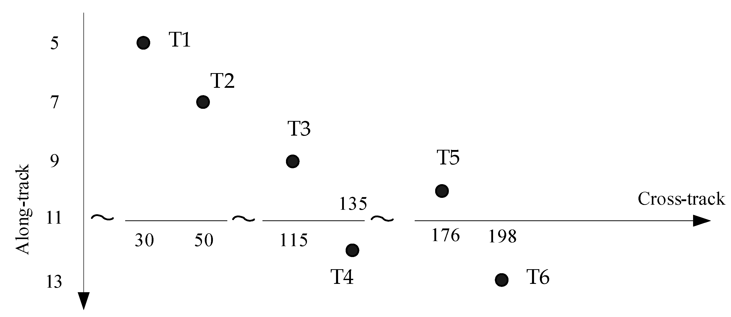
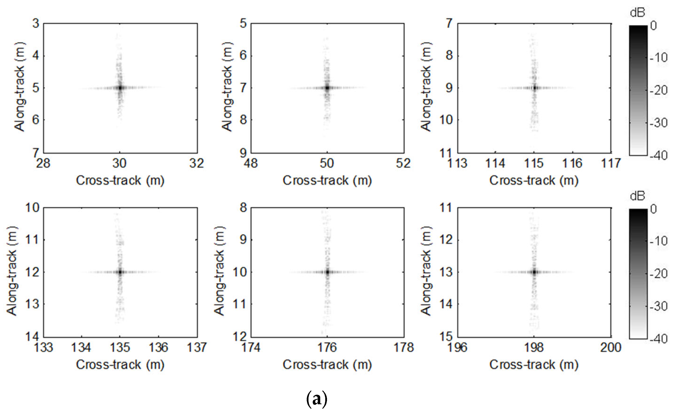
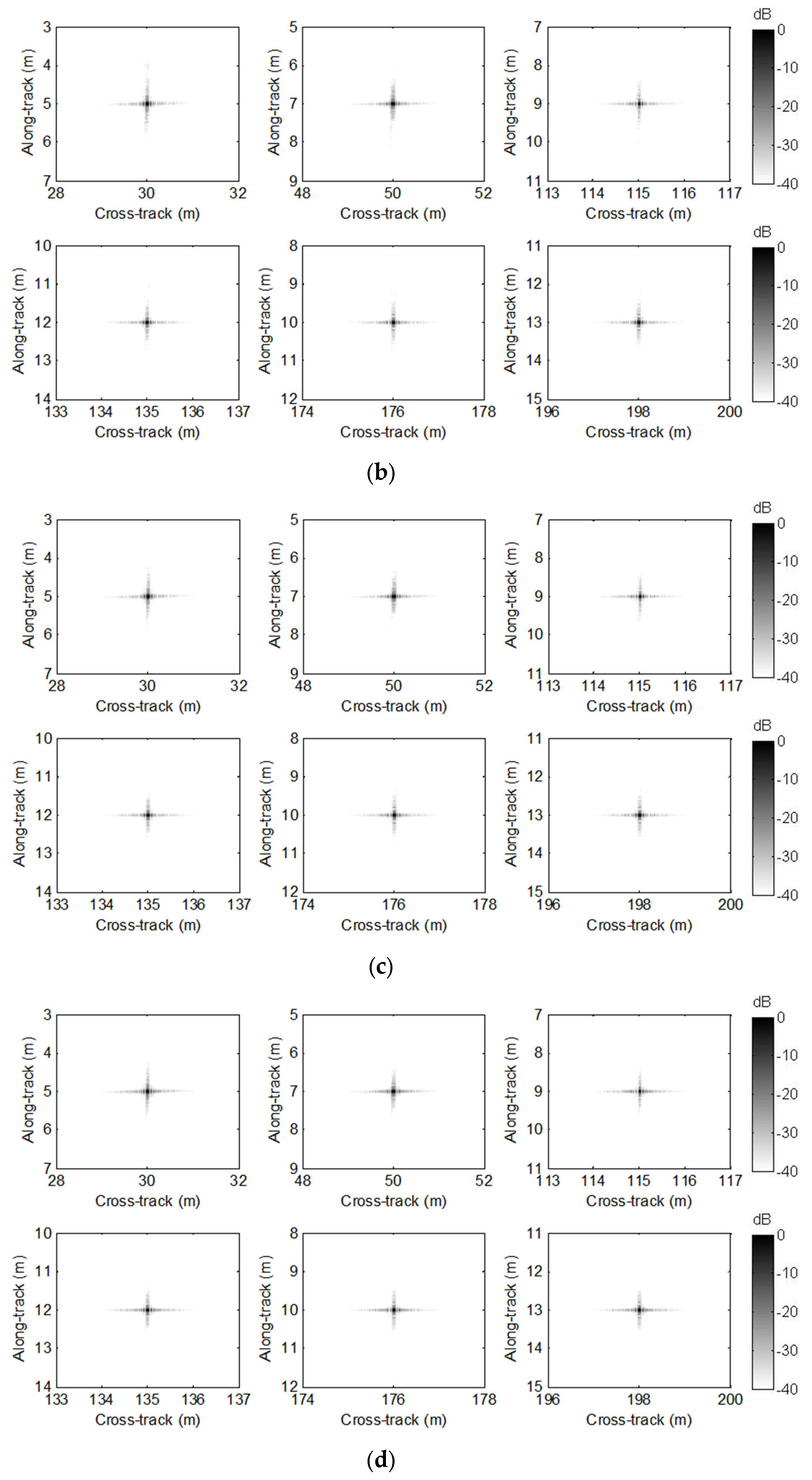
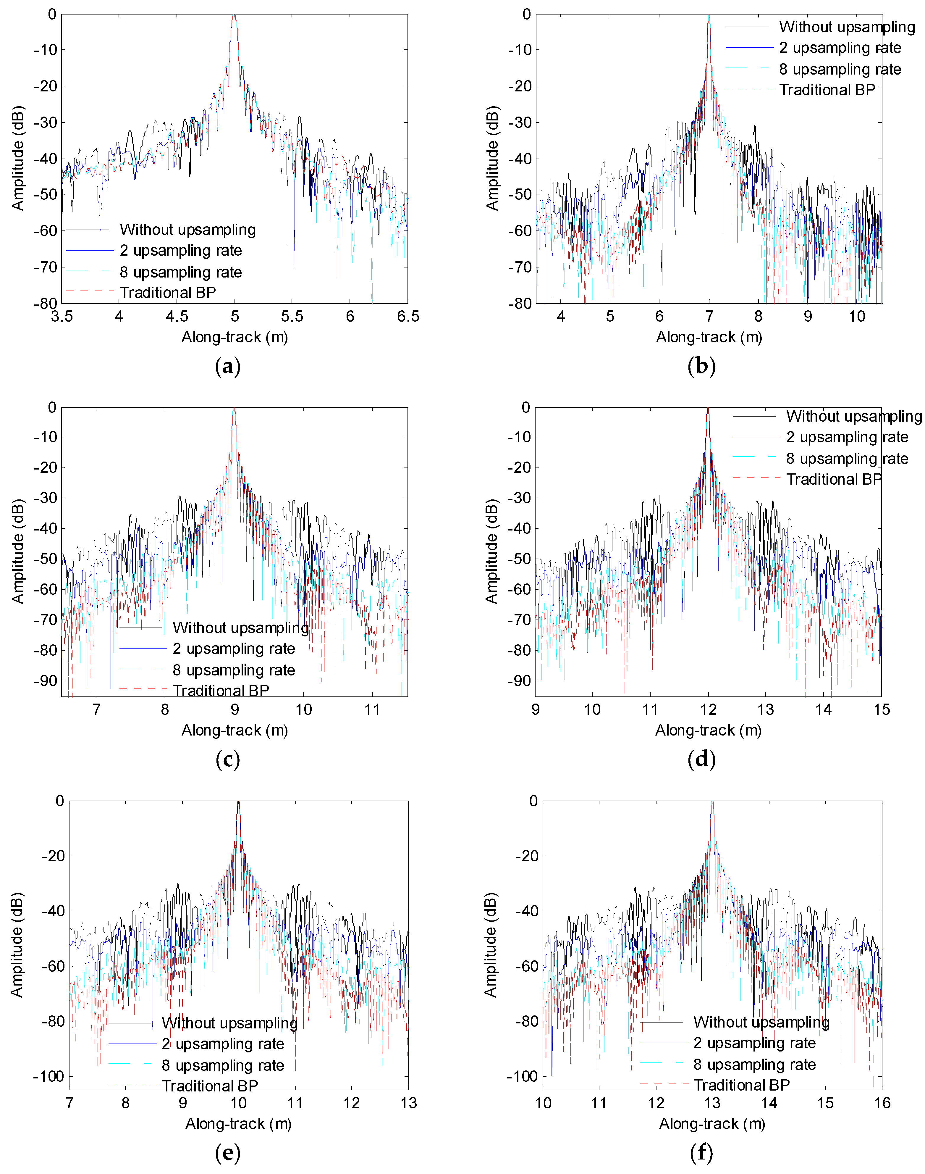
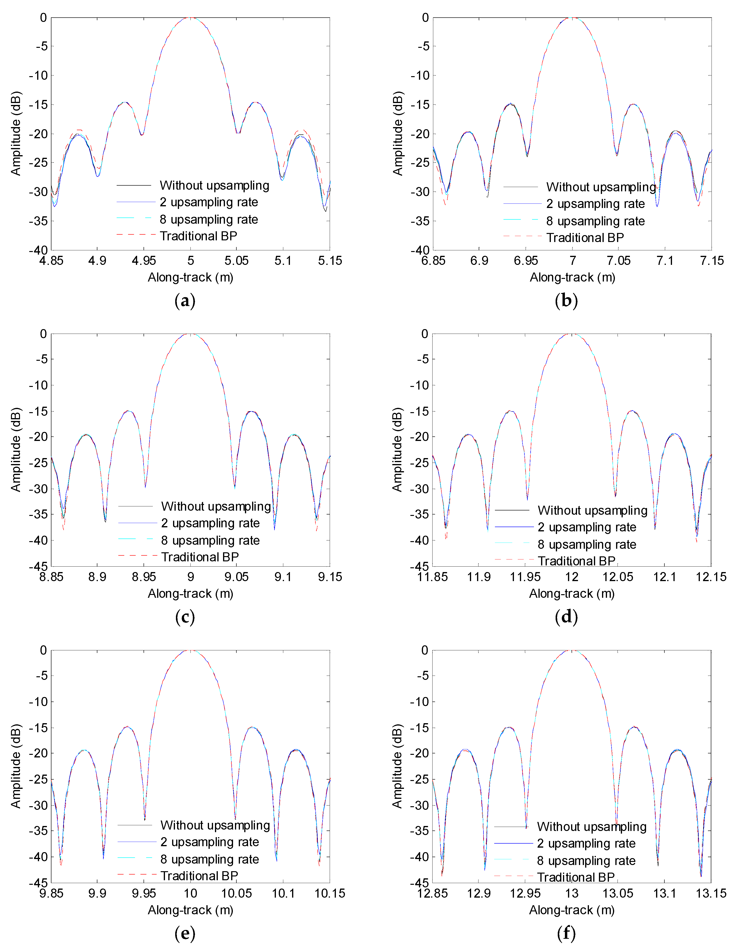
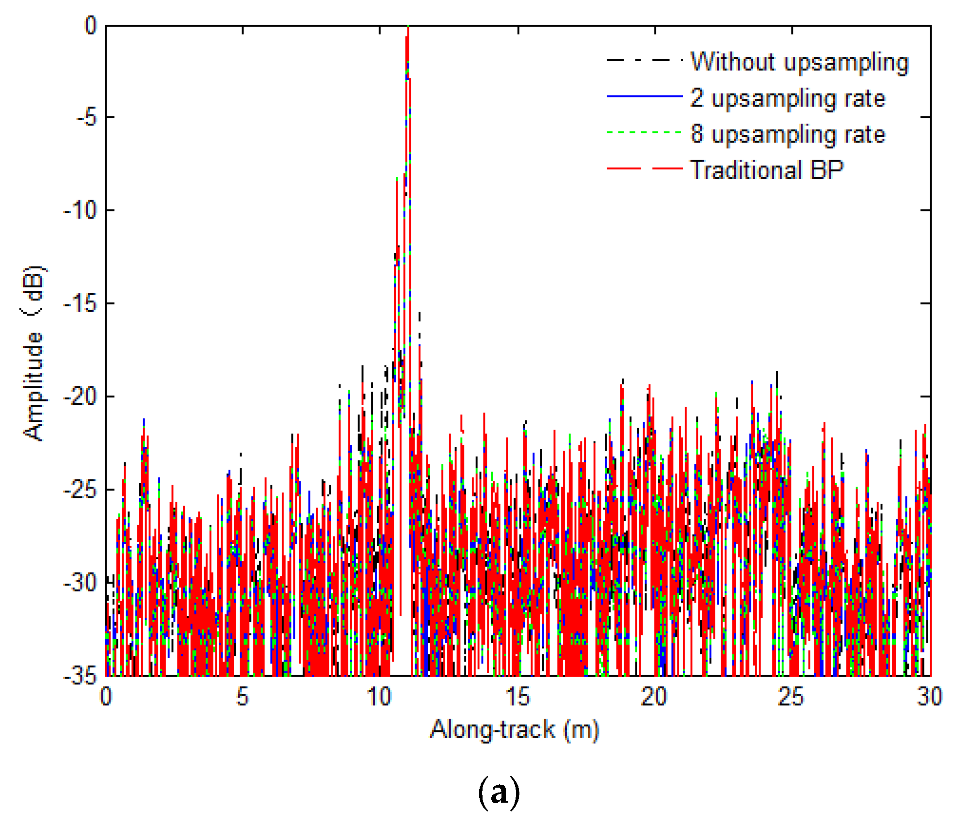
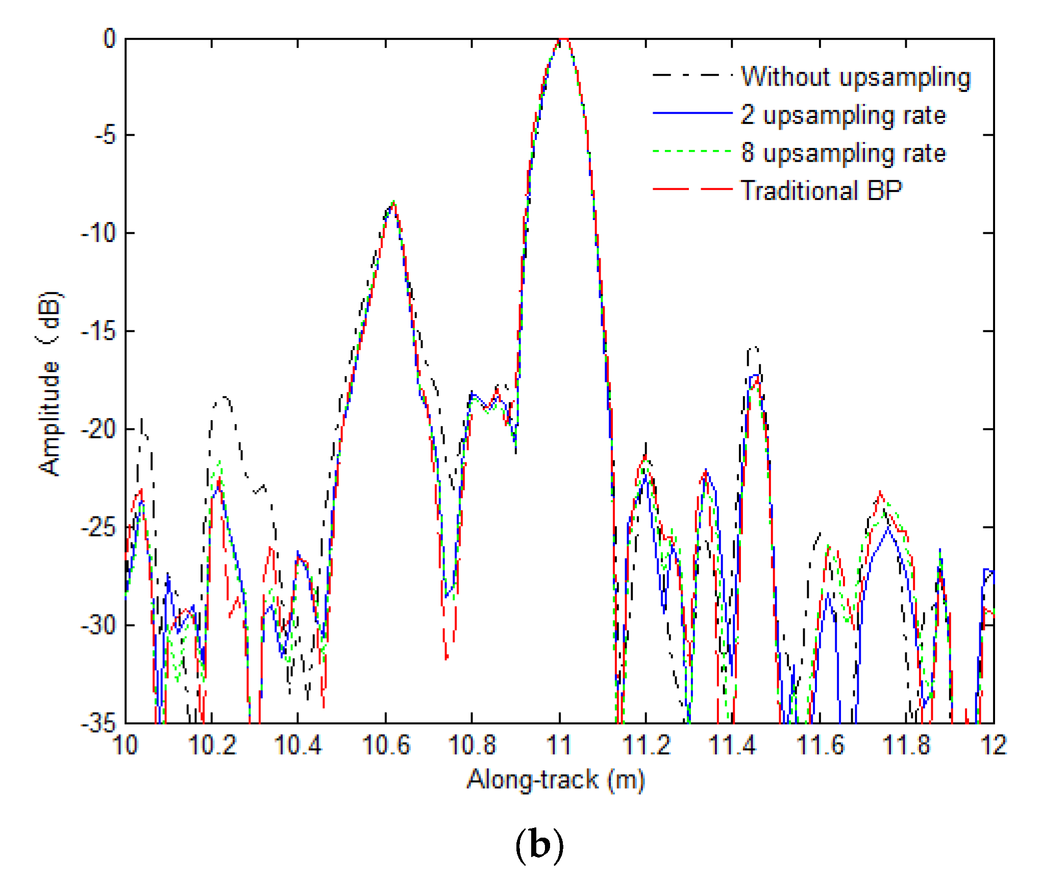
4.1. Simulated Data Processing

The simulations are carried out in this section to validate the presented method. Inspecting Equation (6), the sampling rate highly influences the SAS imaging performance. This section further discusses the influences of the sampling rate on SAS imagery. The SAS parameters are listed in

Table 2. SAS parameters.

Parameter	Value	Unit
Platform velocity	2.5	m/s
Pulse repetition interval	0.32	s
Signal bandwidth	15	kHz
Carrier frequency	150	kHz
Receiver array length	1.6	m
Receiver width	0.04	m
Transmitter width	0.08	m

. Based on Equation (13) and Table 2, we can calculate the minimum upsampling rate $\beta =2$.

We suppose that there are six ideal targets in the imaging scenario, as shown in Figure 7. The targets are marked by T1, T2, … and T6, respectively.

Based on the nearest-neighbor interpolation without an upsampling operation, the imaging results are shown in Figure 8a. When the signal is upsampled using the linear interpolation with upsampling rates of 2 and 8, the results are shown in Figure 8b,c, respectively. For comparison, the data are further processed by the traditional BP algorithm [28] based on sinc-based interpolation, where the kernel length is 8. The results are shown in Figure 8d. Inspecting Figure 8a,d, we find that the results based on the nearest-neighbor interpolation without an upsampling operation has high sidelobes in the along-track dimension. Inspecting Figure 8a,b, the imaging performance based on the presented method with two upsampling rates is highly improved. When we use the presented method with an upsampling rate of 8, the imaging performance is slightly improved compared to that of the presented method with an upsampling rate of 2. In general, the results with the presented method can successfully suppress the high sidelobes shown in Figure 8a.

In order to compare the imaging performance, the slices in the along-track dimension are compared in Figure 9. From Figure 9, the noticeable sidelobes affect the SAS imaging performance when the nearest-neighbor interpolation without an upsampling operation is used. This conclusion is consistent with that drawn from Figure 8a. Fortunately, the sidelobes can be successfully suppressed by utilizing the presented method. However, the sidelobes are still noticeable if the upsampling rate is too low. Fortunately, the imaging performance of the presented method with an upsampling rate of 2 is not noticeably affected. Inspecting the slices of the presented method with an upsampling rate of 8, the imaging performance can be enhanced by improving the upsampling rate.

Figure 10 provides a closer look at the along-track slices shown in Figure 9. The peak sidelobe ratio (PSLR) and along-track resolution can be clearly seen in Figure 10. In general, all imaging methods can obtain almost the same PSLR and along-track resolution. That is to say, the interpolation error mainly influences the sidelobes.

The quality parameters such as the PSLR and integrated sidelobe ratio (ISLR) are calculated in

Table 3. Quality parameters of focused targets.

Method	PLSR (dB)	ISLR (dB)	Target
Nearest interpolation without upsampling	−14.62	−8.08	T1
Presented method with upsampling rate of 2	−14.57	−8.29
Presented method with upsampling rate of 8	−14.58	−8.32
Traditional BP	−14.64	−8.33
Nearest interpolation without upsampling	−15.01	−9.40	T2
Presented method with upsampling rate of 2	−14.83	−9.65
Presented method with upsampling rate of 8	−14.84	−9.77
Traditional BP	−14.87	−9.84
Nearest interpolation without upsampling	−15	−9.62	T3
Presented method with upsampling rate of 2	−14.97	−10.12
Presented method with upsampling rate of 8	−15.0	−10.17
Traditional BP	−14.89	−10.2
Nearest interpolation without upsampling	−15.04	−9.85	T4
Presented method with upsampling rate of 2	−14.98	−10.28
Presented method with upsampling rate of 8	−14.99	−10.41
Traditional BP	−14.94	−10.44
Nearest interpolation without upsampling	−14.94	−9.45	T5
Presented method with upsampling rate of 2	−14.92	−9.79
Presented method with upsampling rate of 8	−14.88	−9.93
Traditional BP	−14.83	−9.96
Nearest interpolation without upsampling	−14.95	−9.52	T6
Presented method with upsampling rate of 2	−14.93	−9.79
Presented method with upsampling rate of 8	−14.89	−9.95
Traditional BP	−14.83	−9.98

. The PSLR [31] is defined by the ratio of the largest level of sidelobes to the peak level of the mainlobe. Here, the mainlobe is defined as the −3 dB width of the along-track slice. PSLR represents the sonar’s ability to identify a weak target from a nearby strong one. The ISLR [31] is the ratio of the total power in all of the sidelobes to the power in the mainlobe. It characterizes the ability to detect weak targets in the neighborhood of bright targets. From Table 3, the PLSR based on the nearest interpolation without upsampling and traditional BP is mostly identical. This conclusion is consistent with that drawn from Figure 6. However, the major difference of ISLR between both methods is 0.59 dB. With the presented method, the imaging performance can be improved. When the presented method with an upsampling rate of 2 is used, the major difference of the ISLR is 0.19 dB compared to the traditional BP algorithm. Furthermore, the imaging performance can be improved by increasing the upsampling rate. When we use the presented method with an upsampling rate of 8, the major difference of the ISLR is just 0.07 dB compared to the traditional BP algorithm. Compared with the presented method with an upsampling rate of 2, the imaging performance is slightly improved when an upsampling rate of 8 is used. This further supports our conclusion discussed in Section 3.3.

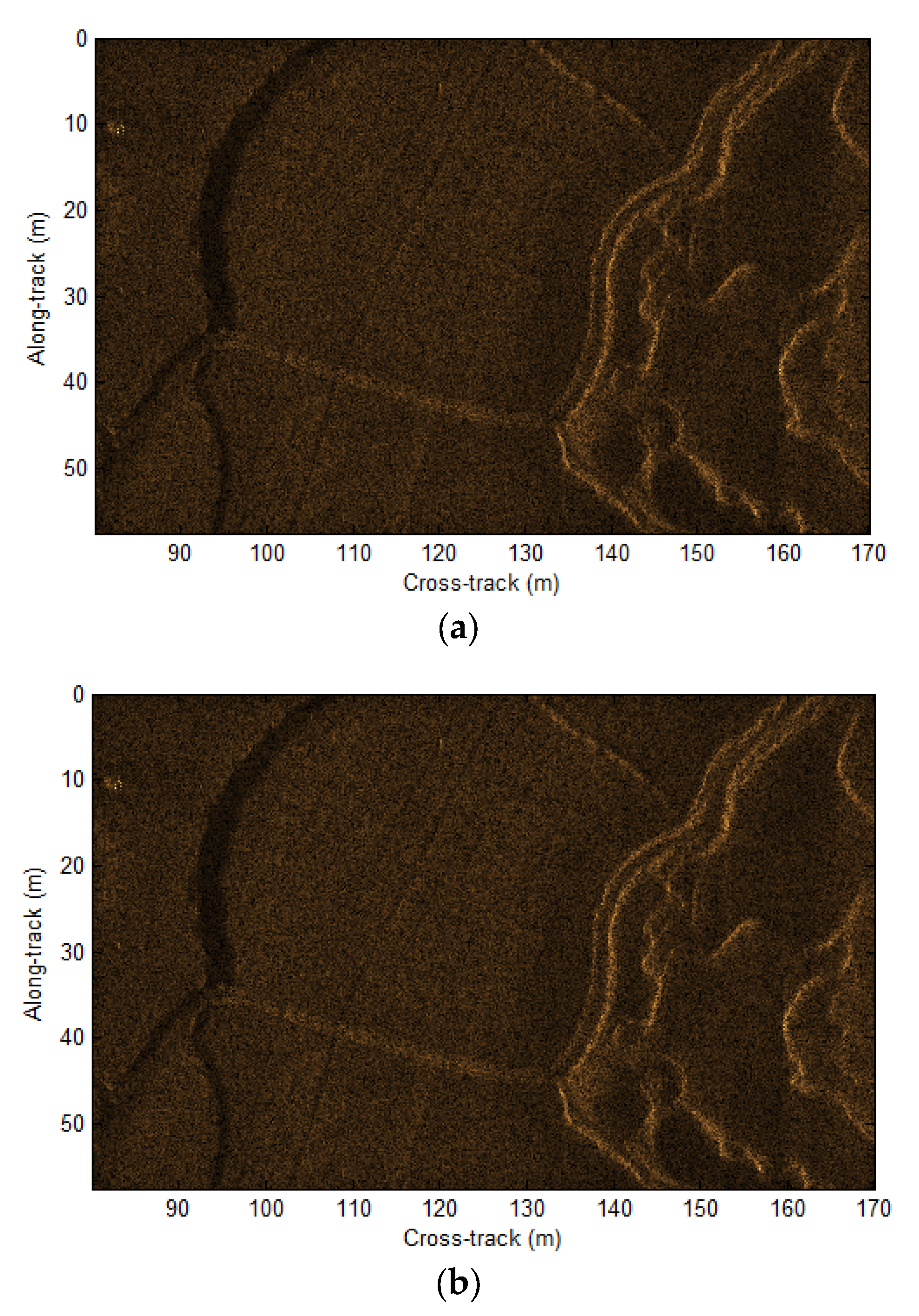
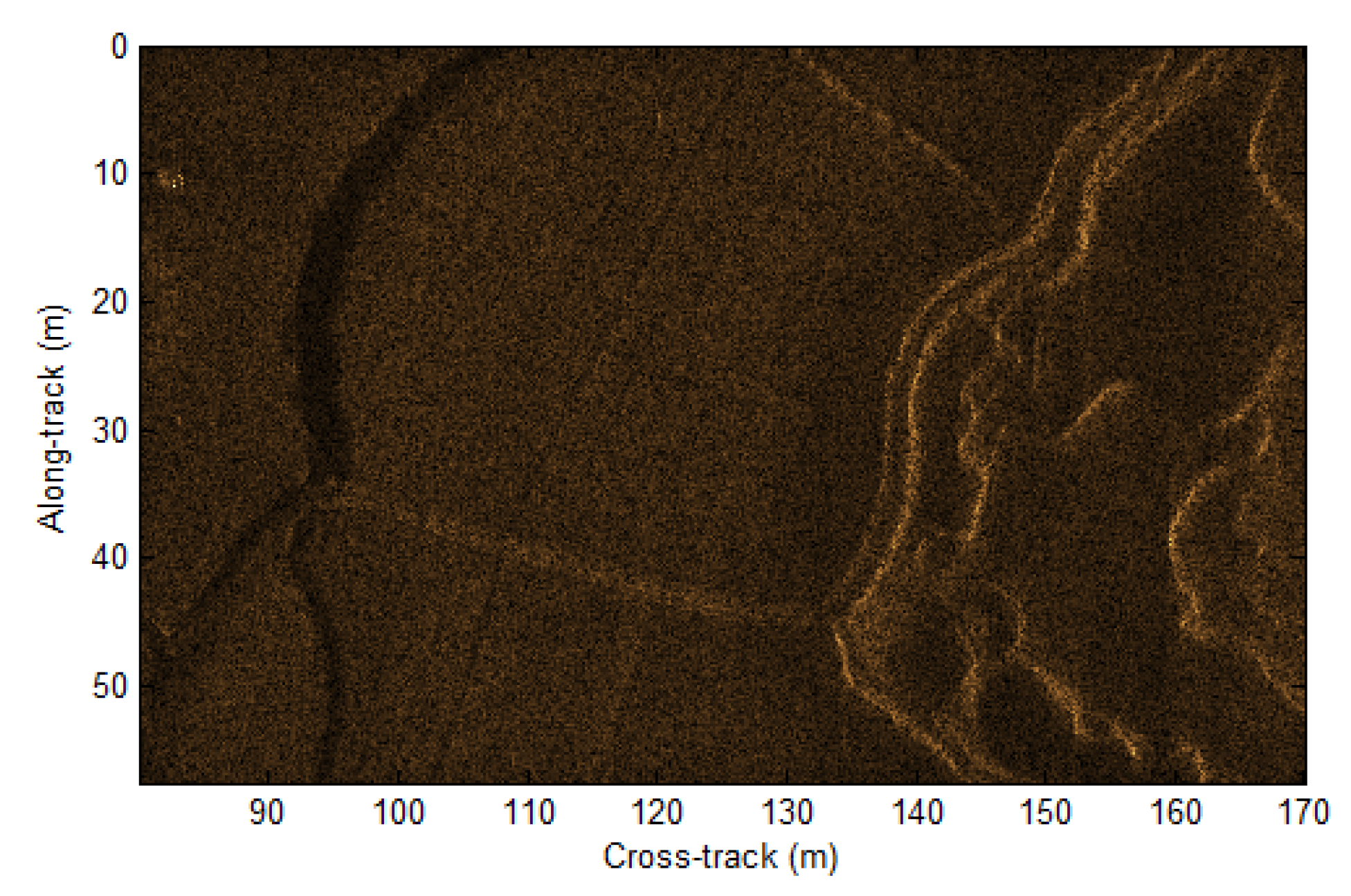
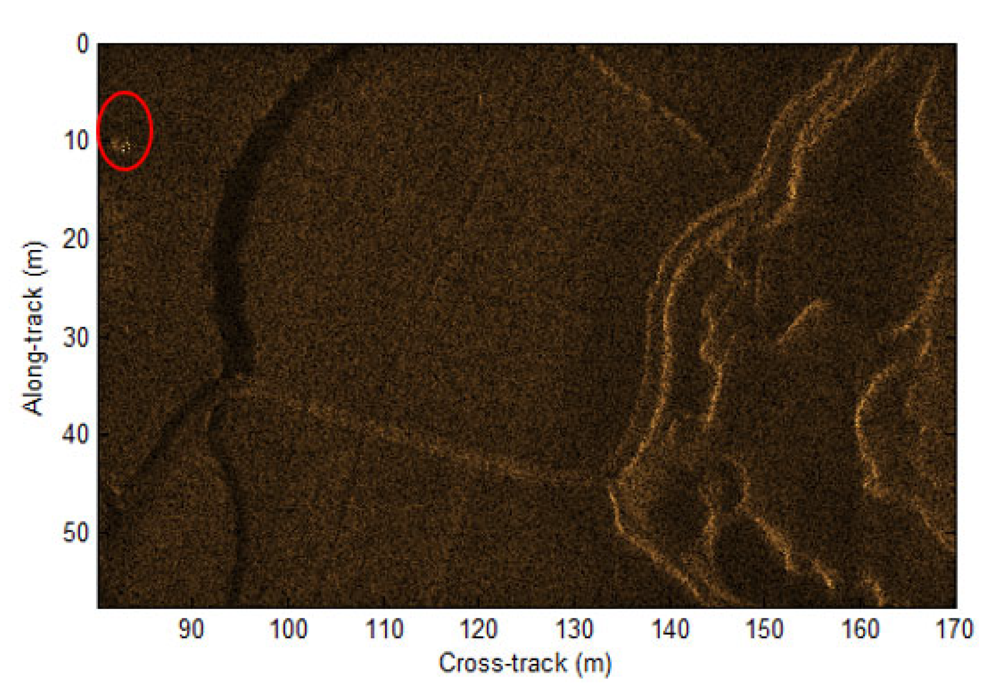
4.2. Real Data Processing

This section validates the presented method based on real data. The data have 2880 sampling points in the along-track dimension and 4800 sampling points in the cross-track dimension. Figure 11 shows the imaging results based on the presented method with upsampling rates of 2 and 8, respectively. For comparison, Figure 12 shows the imaging results using the BP algorithm based on nearest-neighbor interpolation without an upsampling operation. Figure 13 depicts the results based on the traditional BP algorithm [28]. Inspecting Figure 11 and Figure 13, we find that there is little difference between the focusing results based on the presented method, and high-performance images can be obtained in both cases. In practice, the phase error of the presented method with an upsampling rate of 2 is much larger than that with an upsampling rate of 8. When we just obtain the 2D SAS image, this phase error has little influence on the reconstructed image. However, the 2D SAS images are often used to construct three-dimensional (3D) images for Interferometric SAS (InSAS) system. At this point, this phase error would affect the performance of the InSAS image. Inspecting Figure 12 and Figure 13, we find that the BP algorithm based on nearest-neighbor interpolation without an upsampling operation can also obtain similar results. In fact, the interpolation error can seriously influence the InSAS performance, and it must be compensated for when it comes to InSAS processing.

To visually compare the focusing performance, we now concentrate on the along-track slices of the focused target marked by the red circle in Figure 13. The along-track slices are depicted in Figure 14. Figure 14a shows the global slices, while Figure 14b depicts the close-look slices. Figure 14 shows that the slice corresponding to the nearest-neighbor interpolation method without upsampling deviates from that of the traditional BP algorithm. In other words, the interpolation error has influenced the imaging performance. Based on the presented method, the imaging performance can be improved, and the slices of both cases mostly agree well with the slice from the traditional BP algorithm. This further indicates that the presented method can reconstruct the targets well.

The last experiment focuses on the processing time. The processing time of focusing algorithms is listed in

Table 4. Processing time of different focusing algorithms.

	Nearest Interpolation without Upsampling	Presented Method		Traditional BP
		Upsampling Rate of 2	Upsampling Rate of 8
Processing time/s	7156	7368	7420	31,276

, and all algorithms are run on the same computers with MATLAB 2012a. From Table 4, we find that the efficiency of the presented method can be improved 4.22 times in comparison with the traditional BP algorithm. Inspecting Table 1, we find that the time-consuming operation just lies in the complex multiplication. The computation load of linear interpolation is far less than the multiplication. At this point, the nearest-neighbor interpolation method without upsampling, together with the presented method based on upsampling rates of 2 and 8, has almost the same processing time (Table 4). Considering the traditional BP algorithm [31], the computation load of sinc interpolation for N_a and N_r pixels in the along-track and cross-track dimensions is $2(2\alpha -1)N_a^2{N}_r$. Here, $\alpha$ is the length of the interpolator kernel function. For this reason, the traditional BP algorithm is very time-consuming. The efficiency of the presented method can be further improved when lower-performance hardware such as GPU, CUDA, or FPGA are used. With our method, the performance demand for hardware can be significantly decreased. This characteristic is very important for economical users.

5. Conclusions

Due to the range migration between the along-track and cross-track dimensions, the compression in the along-track dimension cannot be directly performed; therefore, the range migration should be corrected first. However, the direct correction based on the nearest-neighbor interpolation method without upsampling leads to a large phase error, which would seriously affect the SAS imaging performance. In this paper, the raw data are first upsampled using the linear interpolation method. Then, the nearest-neighbor interpolation method is used, estimating the data at the desired moment by assigning the data value of the nearest sample as estimated data. The presented method exploits two interpolations, i.e., linear interpolation and nearest neighbor interpolation. With this operation, the interpolation error can be decreased, and the imaging performance can be improved. Furthermore, the computation load of the presented method is not increased, since the linear interpolation just uses adjacent sampled data to estimate the desired value. Based on presented method, the efficiency is lowered in comparison with the traditional BP algorithm based on sinc interpolation. When the presented method is conducted with the lower-performance hardware of CUDA, FPGA, and GPU, it can be expected that the performance of presented method can be further improved. It has great potential to be used for the real-time imagery of multi-receiver SAS systems.

References

1. Rolt, K.D. Ocean, Platform, and Signal Processing Effects on Synthetic Aperture Sonar Performance; Massachusetts Institute of Technology: Cambridge, MA, USA, 1991. [Google Scholar]
2. Pailhas, Y.; Dugelay, S.; Capus, C. Impact of temporal Doppler on synthetic aperture sonar imagery. J. Acoust. Soc. Am. 2018, 143, 318–329. [Google Scholar] [CrossRef]
3. Tan, C.; Zhang, X.; Yang, P.; Sun, M. A novel sub-bottm profiler and signal processor. Sensors 2019, 19, 5052. [Google Scholar] [CrossRef] [Green Version]
4. Maurya, H.; Kumar, A.; Mishra, A.K.; Panigrahi, R.K. Improved four-component based polarimetric synthetic aperture radar image decomposition. IET Radar Sonar Navig. 2020, 14, 619–627. [Google Scholar] [CrossRef]
5. Nithirochananont, U.; Antoniou, M.; Chemiakov, M. Passive coherent multistatic SAR using spaceborne illuminators. IET Radar Sonar Navig. 2020, 14, 628–636. [Google Scholar] [CrossRef]
6. Zhang, X.; Gu, H.; Su, W. Squint-minimised chirp scaling algorithm for bistatic forward-looking SAR imaging. IET Radar Sonar Navig. 2020, 14, 290–298. [Google Scholar] [CrossRef]
7. AlShaya, M.; Yaghoobi, M.; Mulgrew, B. Ultrahigh resolution wide swath MIMO-SAR. IEEE J. Sel. Top. Appl. Earth Obs. Remote Sens. 2020, 13, 5358–5368. [Google Scholar] [CrossRef]
8. Pirrone, D.; Bovolo, F.; Bruzzone, L. An approach to unsupervised detection of fully and partially destroyed buildings in multitemporal VHR SAR images. IEEE J. Sel. Top. Appl. Earth Obs. Remote Sens. 2020, 13, 5938–5953. [Google Scholar] [CrossRef]
9. Wijayasiri, A.; Banerjee, T.; Ranka, S.; Sahni, S.; Schmalz, M. Multiobjective optimization of SAR reconstruction on hybrid multicore systems. IEEE J. Sel. Top. Appl. Earth Obs. Remote Sens. 2020, 13, 4674–4688. [Google Scholar] [CrossRef]
10. Corbett, B.; Andre, D.; Finnis, M. Localising vibrating scatterer phenomena in synthetic aperture radar imagery. Electron. Lett. 2020, 56, 395–398. [Google Scholar] [CrossRef] [Green Version]
11. Hashempour, H.R. Fast ADMM-based approach for high-resolution ISAR imaging. Electron. Lett. 2020, 56, 954–957. [Google Scholar] [CrossRef]
12. Saqueb, S.; Nahar, N.K.; Sertel, K. Fast two-dimensional THz imaging using rail-based synthetic aperture radar (SAR) processing. Electron. Lett. 2020, 56, 988–990. [Google Scholar] [CrossRef]
13. Yang, J.; Qiu, X.; Zhong, L.; Shang, M.; Ding, C. A simultaneous imaging scheme of stationary clutter and moving targets for maritime scenarios with the first Chinese dual-channel spaceborne SAR sensor. Remote Sens. 2019, 11, 2275. [Google Scholar] [CrossRef] [Green Version]
14. Loffeld, O.; Nies, H.; Peters, V.; Knedlik, S. Models and useful relations for bistatic SAR processing. IEEE Trans. Geosci. Remote Sens. 2004, 42, 2031–2038. [Google Scholar] [CrossRef]
15. Zhang, X.; Yang, P. An improved imaging algorithm for multireceiver SAS system with wide-bandwidth signal. Remote Sens. 2021, 13, 5008. [Google Scholar] [CrossRef]
16. Rosu, F.; Anghel, A.; Cacoveanu, R.; Rommen, B.; Datcu, M. Multiaperture focusing for spaceborne transmitter/ground-based receiver bistatic SAR. IEEE J. Sel. Top. Appl. Earth Obs. Remote Sens. 2020, 13, 5823–5832. [Google Scholar] [CrossRef]
17. Callow, H.J. Signal Processing for Synthetic Aperture Sonar Image Enhancement; University of Canterbury: Christchurch, New Zealand, 2003. [Google Scholar]
18. Gough, P.T.; Hayes, M.P. Fast Fourier techniques for SAS imagery. In Proceedings of the MTS/IEEE Oceans Conference, Brest, France, 20–23 June 2005; pp. 563–568. [Google Scholar]
19. Zhang, X.; Wu, H.; Sun, H.; Ying, W. Multireceiver SAS imagery based on monostatic conversion IEEE J. Sel. Top. Appl. Earth Obs. Remote Sens. 2021, 14, 10835–10853. [Google Scholar] [CrossRef]
20. Bonifant, W.W.; Richards, M.; McClellan, J. Interferometric height estimation of the seafloor via synthetic aperture sonar in the presence of motion errors. IEE Proc. Radar Sonar Navig. 2000, 147, 322–330. [Google Scholar] [CrossRef] [Green Version]
21. Vu, V.T.; Sjogren, T.K.; Pettersson, M.I. Two-dimensional spectrum for BiSAR derivation based on Lagrange inversion theorem. IEEE Geosci. Remote Sens. Lett. 2014, 11, 1210–1214. [Google Scholar] [CrossRef] [Green Version]
22. Neo, Y.L.; Wong, F.; Cumming, I.G. A two-dimensional spectrum for bistatic SAR processing using series reversion. IEEE Geosci. Remote Sens. Lett. 2007, 4, 93–96. [Google Scholar] [CrossRef]
23. Zhang, X.; Yang, P.; Dai, X. Focusing the multireceiver SAS data based on the fourth order Legendre expansion. Circuits Syst. Signal Process. 2019, 38, 2607–2629. [Google Scholar] [CrossRef]
24. Wu, J.J.; Yang, J.Y.; Huang, Y.L.; Liu, Z.; Yang, H.G. A new look at the point target reference spectrum for bistatic SAR. Prog. Electromagn. Res. 2011, 119, 363–379. [Google Scholar] [CrossRef] [Green Version]
25. Wang, F.; Li, X. A new method of deriving spectrum for bistatic SAR processing. IEEE Geosci. Remote Sens. Lett. 2010, 7, 483–486. [Google Scholar] [CrossRef]
26. Yang, H.L.; Tang, J.S.; Li, Q.H.; Liu, X.D. A robust multiple-receiver Range-Doppler algorihtm for synthetic aperture sonar imagery. In Proceedings of the MTS/IEEE Oceans Conference, Aberdeen, UK, 18–21 June 2007; pp. 1–5. [Google Scholar]
27. Bamler, R.; Meyer, F.; Liebhart, W. Processing of bistatic SAR data from quasi-stationary configurations. IEEE Trans. Geosci. Remote Sens. 2007, 45, 3350–3358. [Google Scholar] [CrossRef]
28. Duersch, M.I. Backprojection for Synthetic Aperture Radar; Brigham Young University: Provo, UT, USA, 2013. [Google Scholar]
29. Wang, X.; Zhang, X.; Zhu, S. Upsampling based back projection imaging algorithm for multi-receiver synthetic aperture sonar. In Proceedings of the 2015 International Industrial Informatics and Computer Engineering Conference (IIICEC), Xi’an, China, 10–11 January 2015; pp. 1610–1615. [Google Scholar]
30. Zhang, M.; Wang, G.; Zhang, L. Precise aperture-dependent motion compensation with frequency domain fast back-projection algorithm. Sensors 2017, 17, 2454. [Google Scholar] [CrossRef] [Green Version]
31. Cumming, I.; Wong, F. Digtal Processing of Synthetic Aperture Radar Data: Algorithms and Implementation; Artech House: Norwood, MA, USA, 2005. [Google Scholar]
32. Zhang, X.; Yang, P.; Ying, W. BP algorithm for the multireceiver SAS system. IET Radar Sonar Navig. 2019, 13, 830–838. [Google Scholar] [CrossRef]
33. Li, X.; Zhou, S.; Yang, L. A new fast factorized back-projection algorithm with reduced topography sensibility for missile-borne SAR focusing with diving movement. Remote Sens. 2020, 12, 2616. [Google Scholar] [CrossRef]
34. Liu, W.; Zhang, C.; Liu, J. Application of FFBP algorithm to synthetic aperture sonar imaging. Tech. Acoust. 2009, 28, 572–576. [Google Scholar]
35. Hunter, A.; Hayes, M.; Gough, P. A comparison of fast factorised back-projection and wavenumber algorithms for SAS image reconstruction. In Proceedings of the 5th World Congress on Ultrasonics, Paris, France, 7–10 September 2003; pp. 527–530. [Google Scholar]
36. Shippey, G.; Banks, S.; Pihl, J. SAS image reconstruction using fast polar back projection: Comparisons with fast factored back projection and Fourier-domain imaging. In Proceedings of the Europe Oceans 2005, Brest, France, 20–23 June 2005; pp. 96–101. [Google Scholar]
37. Wu, S.; Xu, Z.; Wang, F.; Yang, D.S.; Guo, G. An improved back-projection algorithm for GNSS-R BSAR imaging based on CPU and GPU platform. Remote Sens. 2021, 13, 2107. [Google Scholar] [CrossRef]
38. Baralli, F.; Couillard, M.; Ortiz, A.; Caldwell, D.G. GPU-based real-time synthetic aperture sonar processing on-board autonomous underwater vehicles. In Proceedings of the 2013 MTS/IEEE Oceans, Bergen, Norway, 10–13 June 2013; pp. 1–8. [Google Scholar]
39. Campbell, D.; Cook, D.A. Using graphics processors to accelerate synthetic aperture sonar imaging via backpropagation. In Proceedings of the High Performance Embedded Computing Workshop (HPEC’ 10), MIT Lincoln Laboratory, Lexington, MA, USA, 19–21 September 2010; pp. 1–3. [Google Scholar]
40. Fasih, A.; Hartley, T. GPU-accelerated synthetic aperture radar backprojection in CUDA. In Proceedings of the 2010 IEEE Radar Conference, Arlington, VA, USA, 10–14 May 2010; pp. 1408–1413. [Google Scholar]
41. Hettiarachchi, D.; Balster, E. Fixed-point processing of the SAR back-projection algorithm on FPGA. IEEE J. Sel. Top. Appl. Earth Obs. Remote Sens. 2021, 14, 10889–10902. [Google Scholar] [CrossRef]
42. Zhang, C. Synthetic Aperture Radar: Principles, System Analysis and Applications; Science Press: Beijing, China, 1989. [Google Scholar]
Figure 1. System model of SAS sampling and imaging.
Jmse 10 00718 g001
Figure 2. Multi-receiver SAS imaging geometry.
Jmse 10 00718 g002
Figure 3. Multi-receiver SAS imaging geometry. (a) Object space; (b) data space; (c) image space.
Jmse 10 00718 g003
Figure 4. Diagram of linear interpolation.
Jmse 10 00718 g004
Figure 5. Block diagram of presented method.
Jmse 10 00718 g005
Figure 6. Block diagram of focus depth.
Jmse 10 00718 g006
Figure 7. Distribution of simulation scene.
Jmse 10 00718 g007
Figure 8. Imaging results with simulated data. (a) Nearest−neighbor interpolation without upsampling operation; (b) presented method with upsampling rate of 2; (c) presented method with upsampling rate of 8; (d) traditional BP algorithm.
Jmse 10 00718 g008aJmse 10 00718 g008b
Figure 9. Along−track slices of focused targets. (a) T1; (b) T2; (c) T3; (d) T4; (e) T5; (f) T6.
Jmse 10 00718 g009
Figure 10. Close look at along−track slices. (a) T1; (b) T2; (c) T3; (d) T4; (e) T5; (f) T6.
Jmse 10 00718 g010
Figure 11. Real-data processing results with presented method. (a) Upsampling rate of 2; (b) upsampling rate of 8.
Jmse 10 00718 g011
Figure 12. Real-data processing result using nearest interpolation without upsampling.
Jmse 10 00718 g012
Figure 13. Real-data processing result with traditional BP algorithm. The area circled by red circle is a reconstructed target, which would be discussed in the following part.
Jmse 10 00718 g013
Figure 14. Along−track slices of target marked by a red circle in Figure 9. (a) Global slices; (b) close look.
Jmse 10 00718 g014aJmse 10 00718 g014b