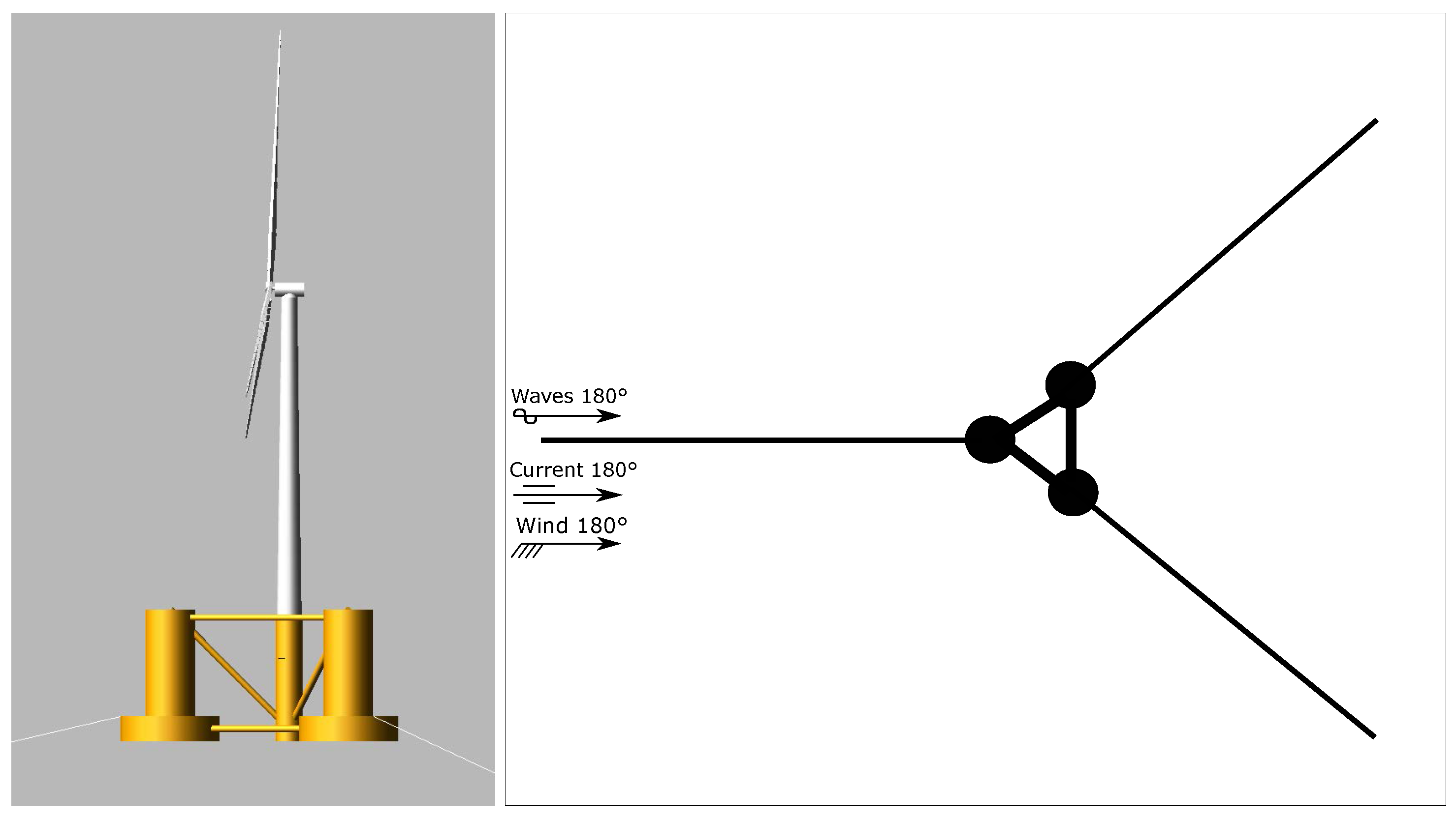
Figure 1.
(
Left) OC4-DeepCWind FOWT design. (
Right) Top view of the mooring system of the OC4-DeepCWind FOWT [
33].
Figure 1.
(
Left) OC4-DeepCWind FOWT design. (
Right) Top view of the mooring system of the OC4-DeepCWind FOWT [
33].
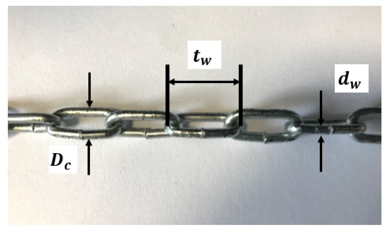
Figure 2.
Principal dimensions of the selected chain.
Figure 2.
Principal dimensions of the selected chain.
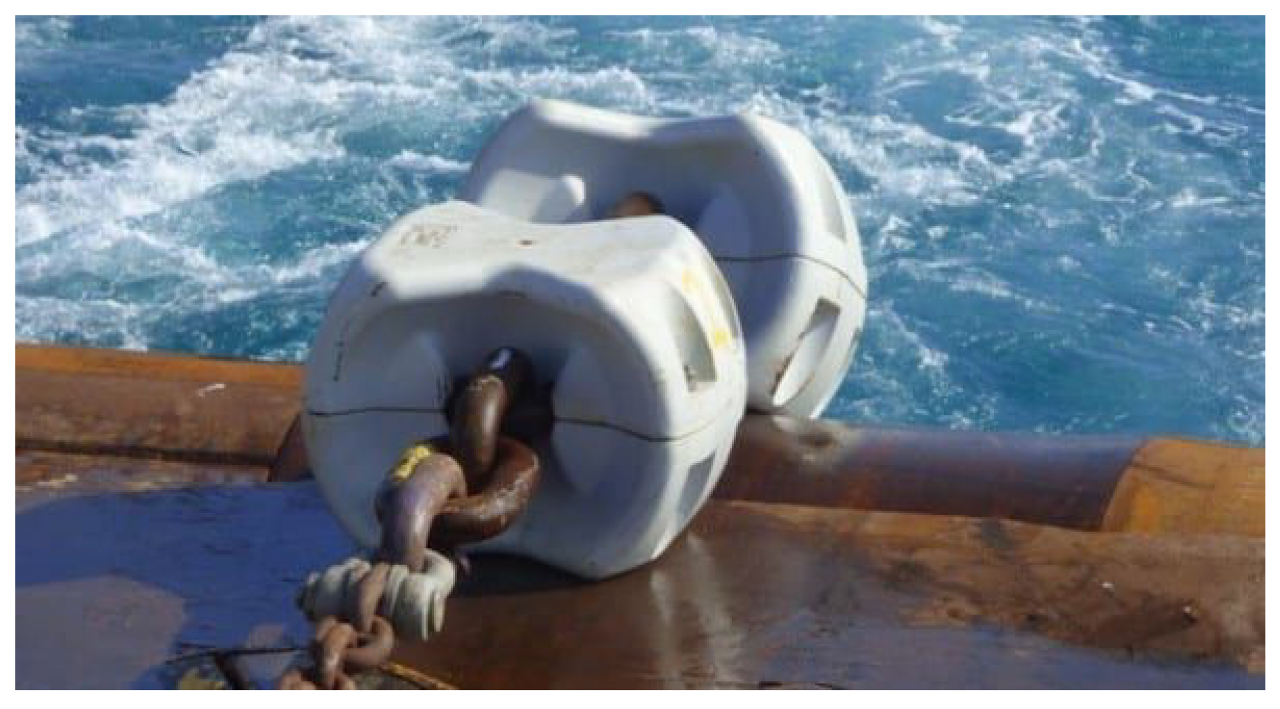
Figure 3.
Typical clumped weight used in the offshore industry.
Figure 3.
Typical clumped weight used in the offshore industry.
Figure 4.
Designed and manufactured scaled clumped weight (left) and snapshot of the clumped weight installed in the mooring line obtained with the submerged camera (right).
Figure 4.
Designed and manufactured scaled clumped weight (left) and snapshot of the clumped weight installed in the mooring line obtained with the submerged camera (right).
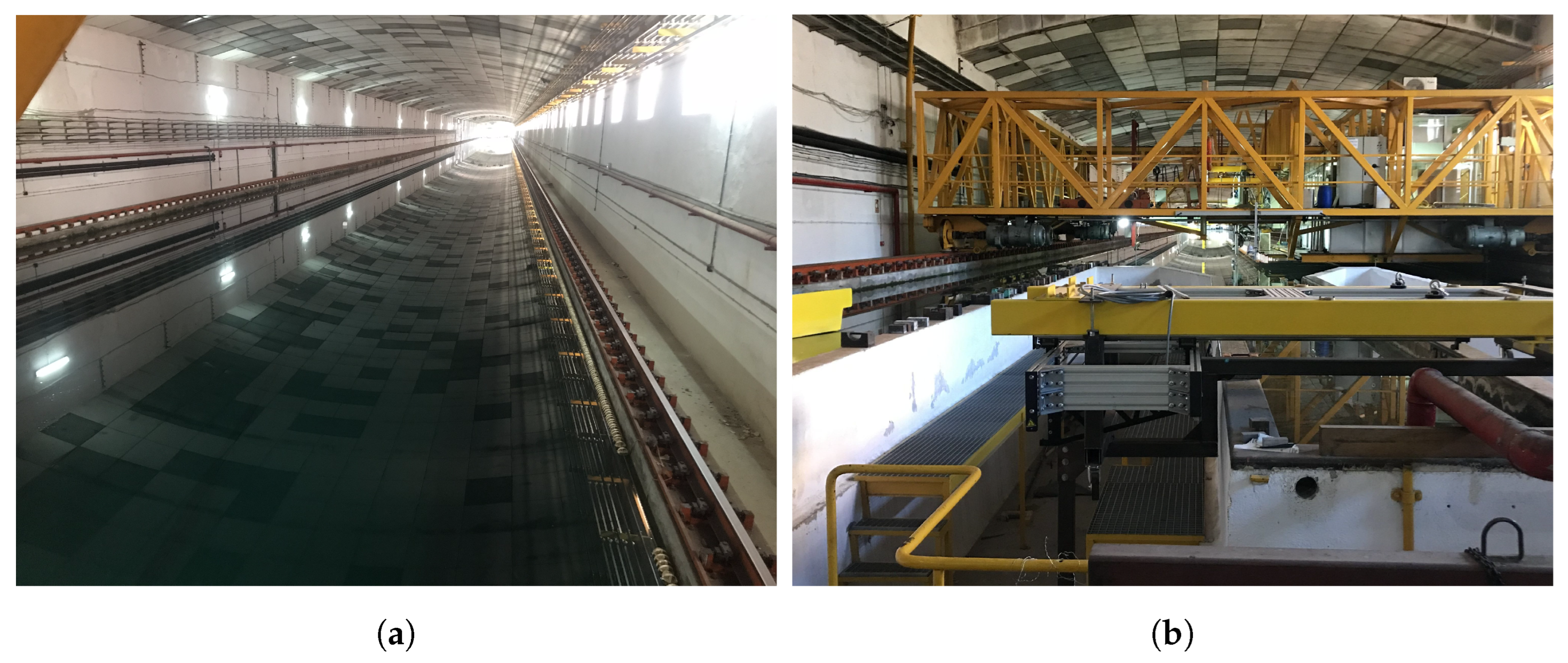
Figure 5.
CEHIPAR facilities. (a) CEHIPAR towing tank. (b) CEHIPAR towing tank carriage.
Figure 5.
CEHIPAR facilities. (a) CEHIPAR towing tank. (b) CEHIPAR towing tank carriage.
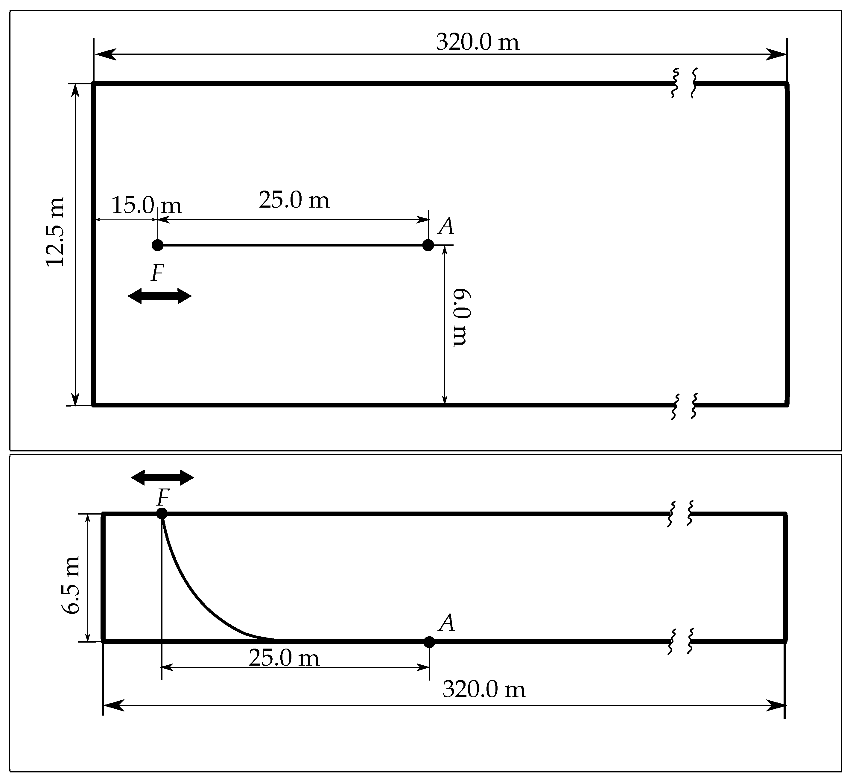
Figure 6.
Schematic layout of the top and side views of the experimental setup.
Figure 6.
Schematic layout of the top and side views of the experimental setup.
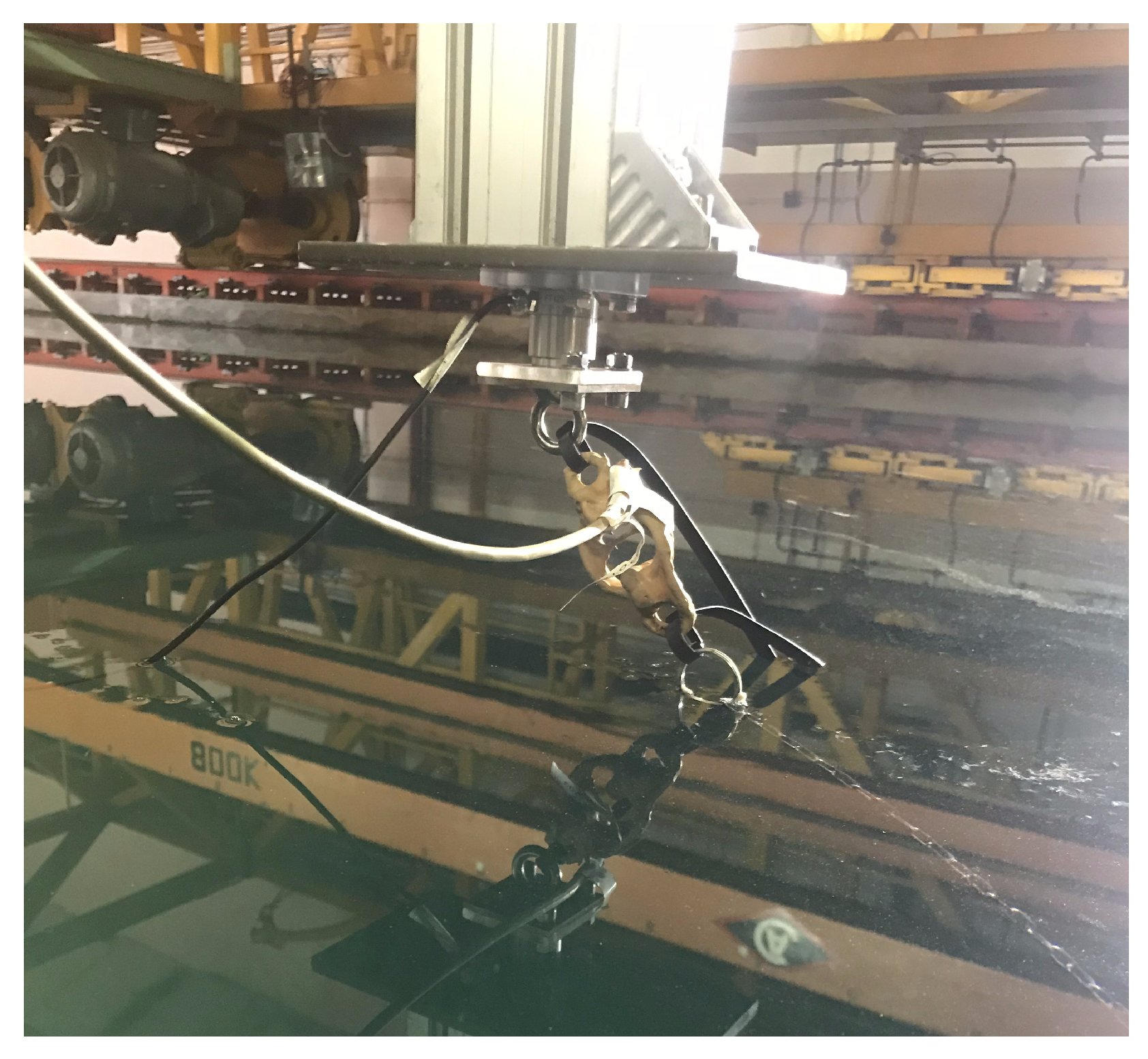
Figure 7.
The load cell and dynamometer connection to the aluminum beam attached to the linear guide.
Figure 7.
The load cell and dynamometer connection to the aluminum beam attached to the linear guide.
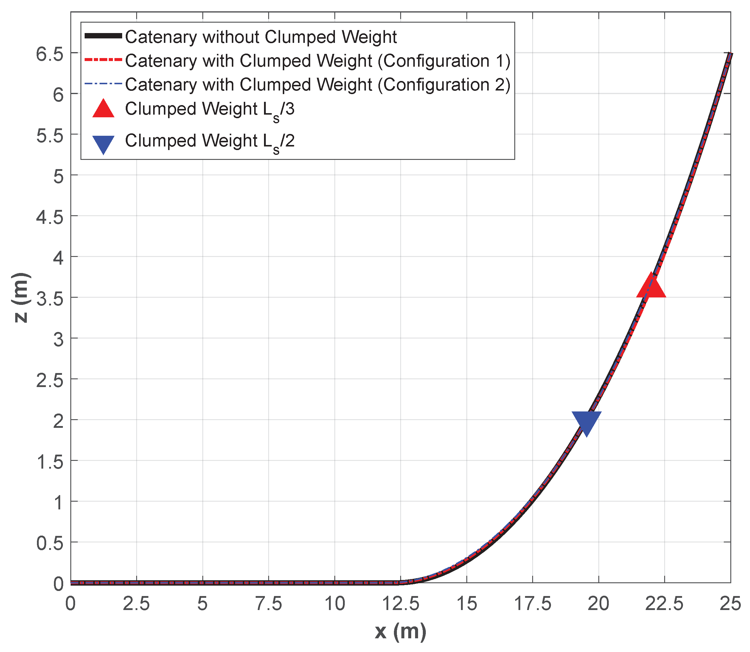
Figure 8.
All three tested configurations. Note: the three lines are almost overlapping, the catenary shape is slightly changed in each configuration.
Figure 8.
All three tested configurations. Note: the three lines are almost overlapping, the catenary shape is slightly changed in each configuration.
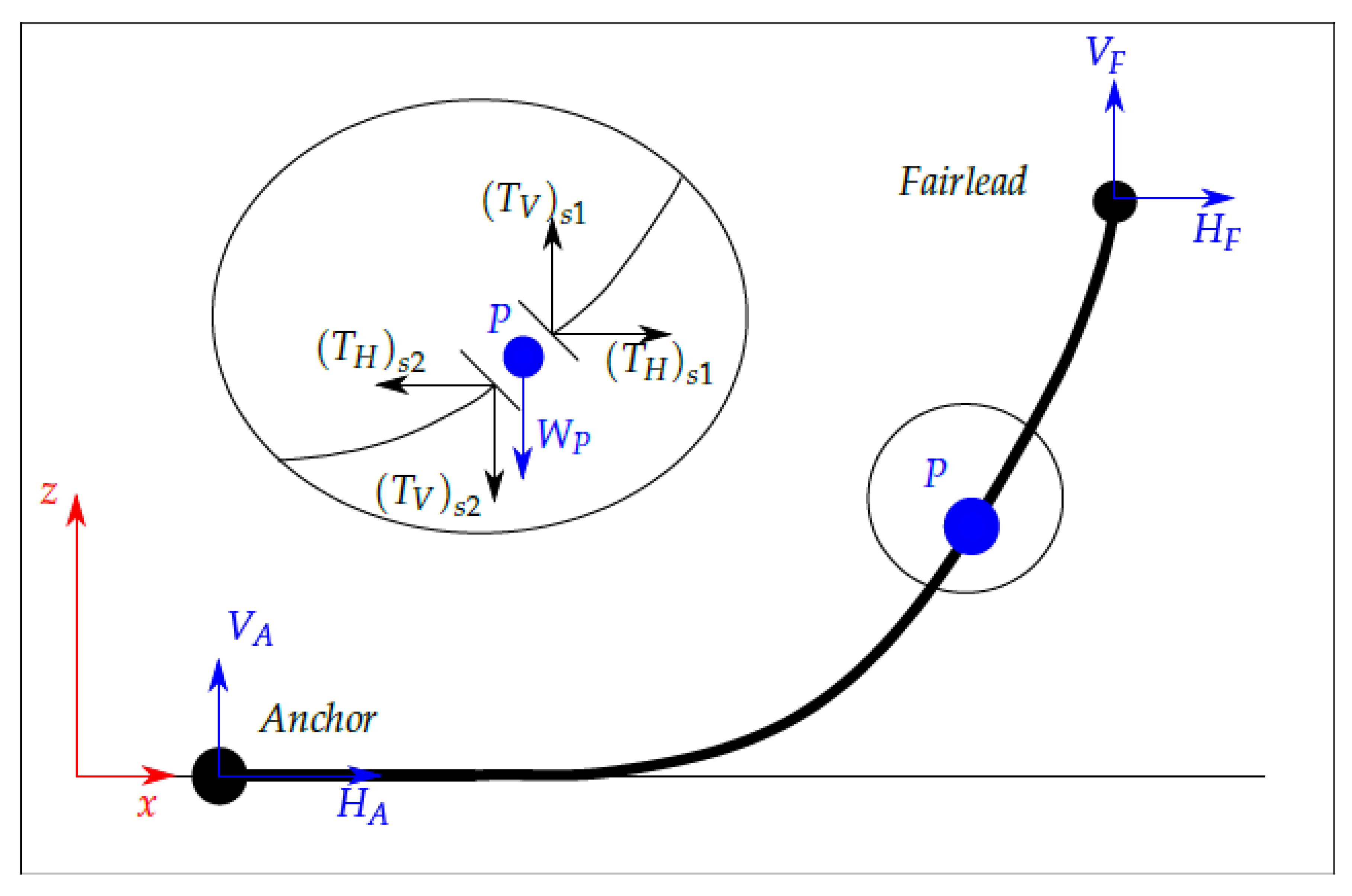
Figure 9.
Free body diagram of a mooring line with a clumped weight positioned at point P.
Figure 9.
Free body diagram of a mooring line with a clumped weight positioned at point P.
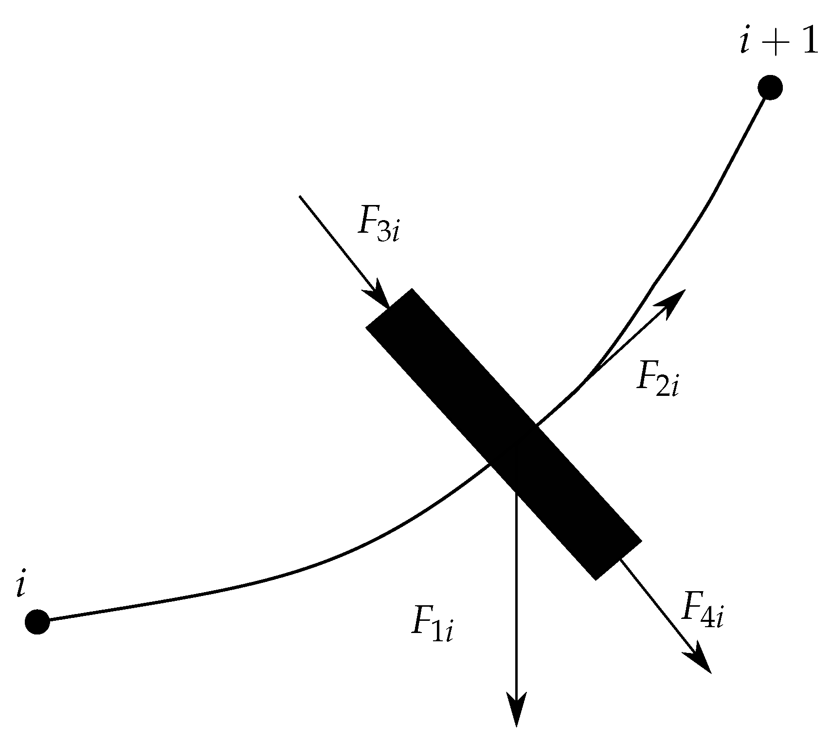
Figure 10.
External forces acting on an element of line.
Figure 10.
External forces acting on an element of line.
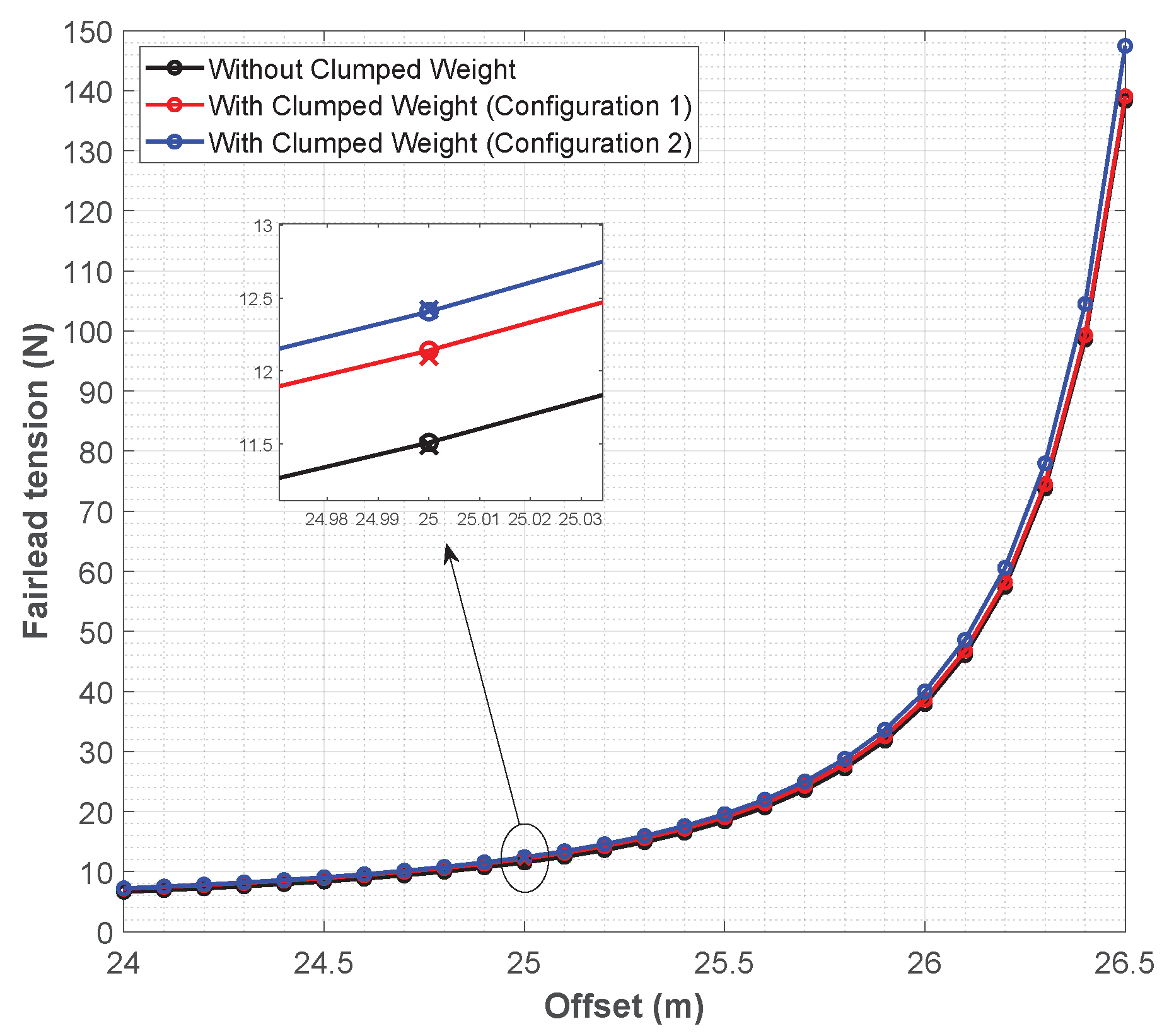
Figure 11.
Variation of the tension with offset distance in all configurations. Experimental values are added to the figure with crossed symbols ‘x’ in the detailed view.
Figure 11.
Variation of the tension with offset distance in all configurations. Experimental values are added to the figure with crossed symbols ‘x’ in the detailed view.
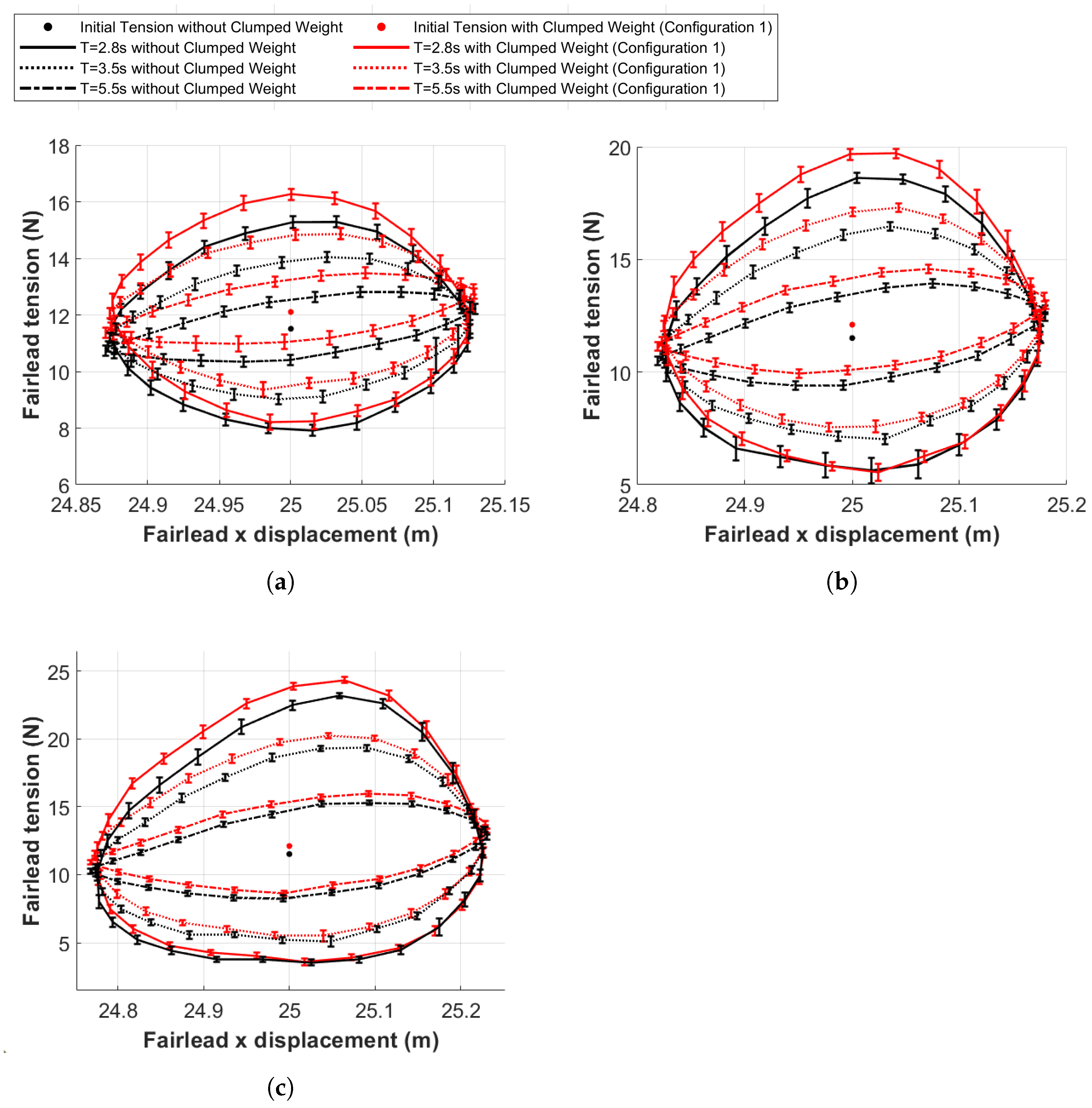
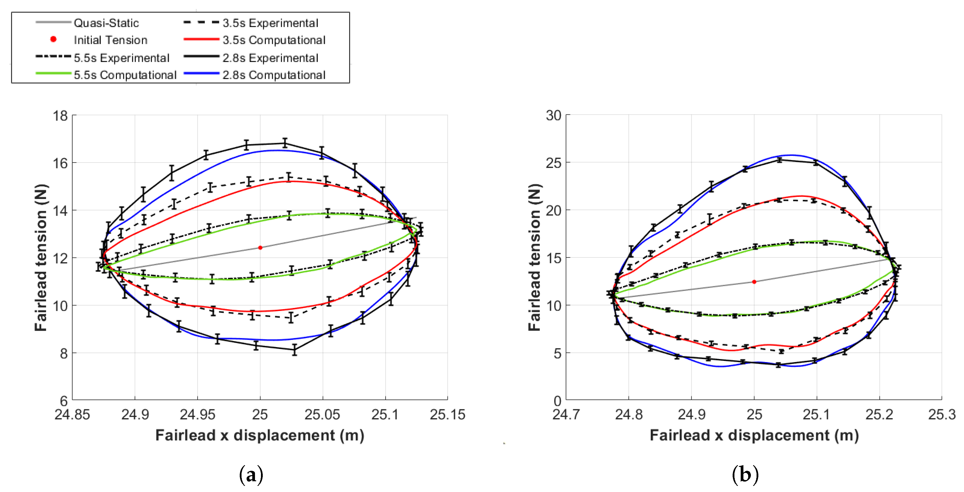
Figure 12.
Fairlead tension during the fairlead displacement with and without clumped weight for three different fairlead amplitude values and Configuration 1. (a) m. (b) m. (c) m.
Figure 12.
Fairlead tension during the fairlead displacement with and without clumped weight for three different fairlead amplitude values and Configuration 1. (a) m. (b) m. (c) m.
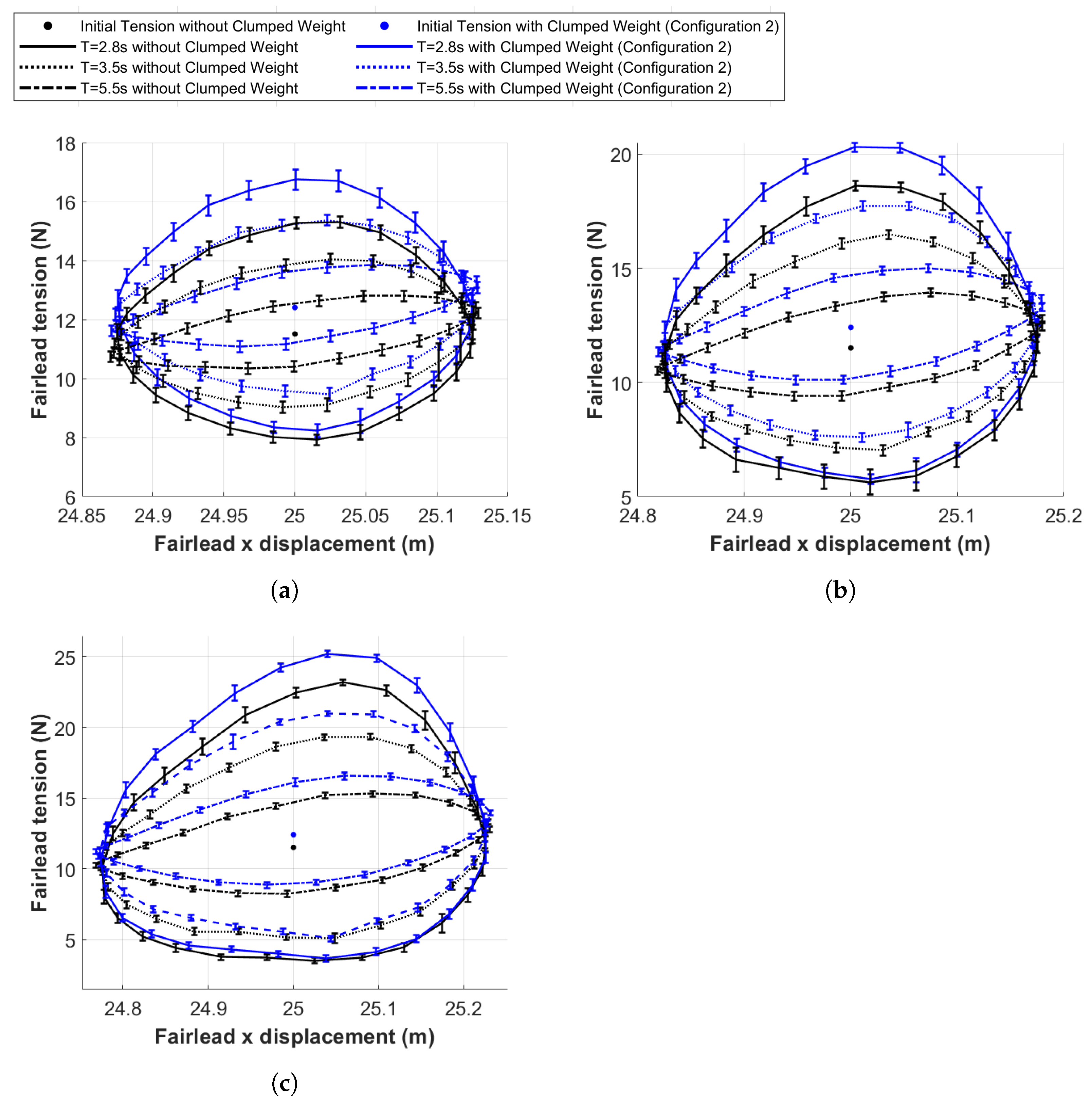
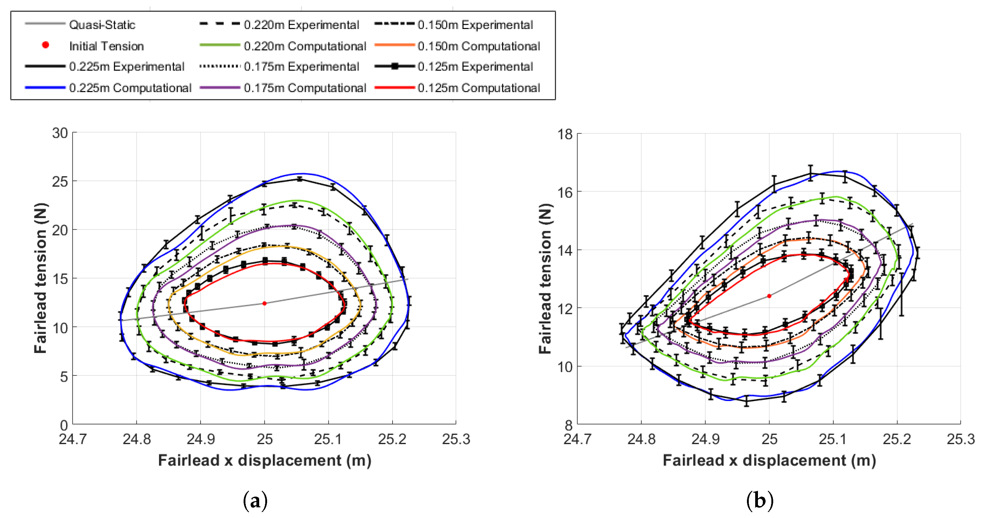
Figure 13.
Fairlead tension during the fairlead displacement with and without clumped weight for three different fairlead amplitude values and Configuration 2. (a) m. (b) m. (c) m.
Figure 13.
Fairlead tension during the fairlead displacement with and without clumped weight for three different fairlead amplitude values and Configuration 2. (a) m. (b) m. (c) m.
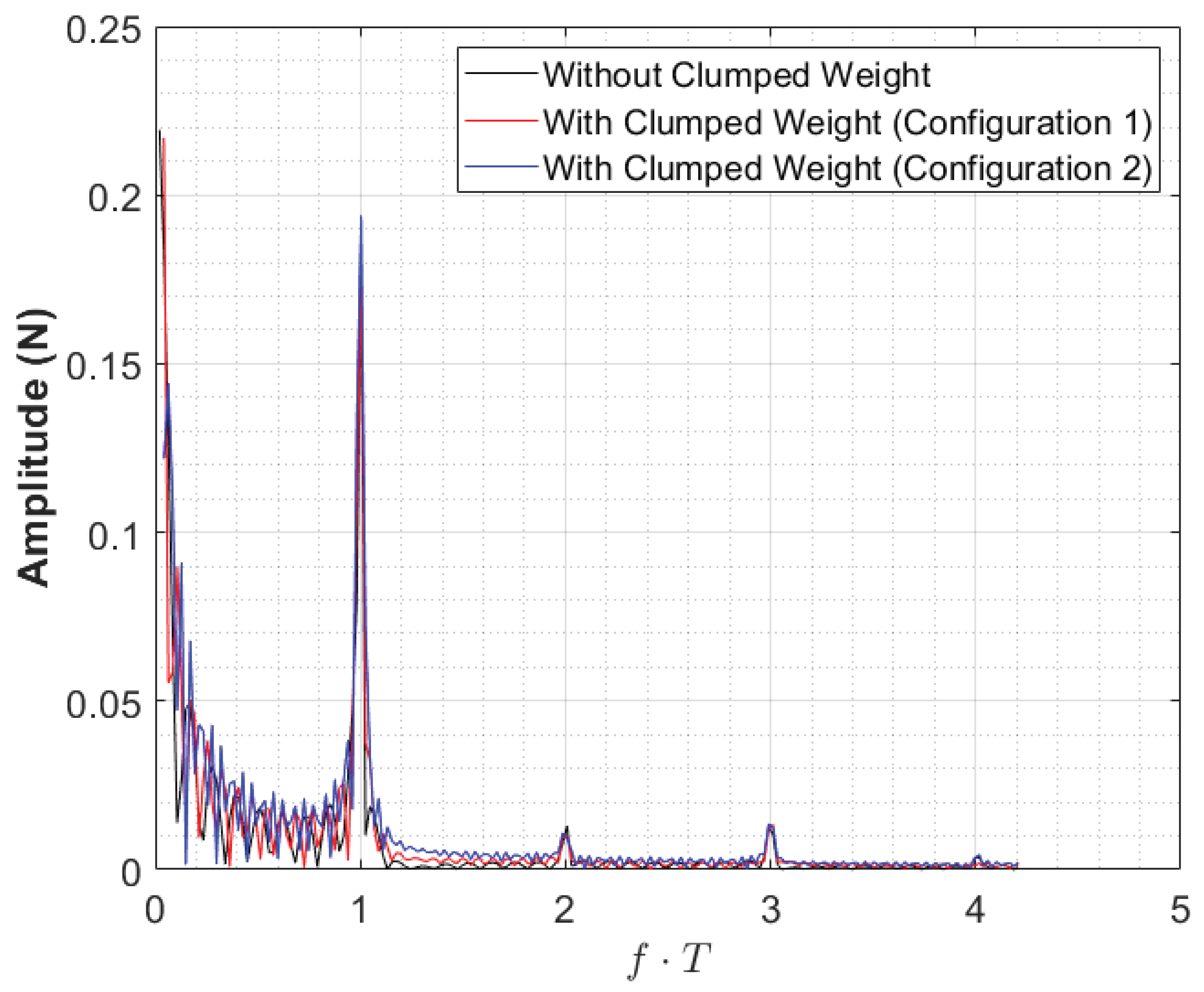
Figure 14.
Spectrum plot of the top-end tensions for an amplitude of s and period s for the three tested configurations.
Figure 14.
Spectrum plot of the top-end tensions for an amplitude of s and period s for the three tested configurations.
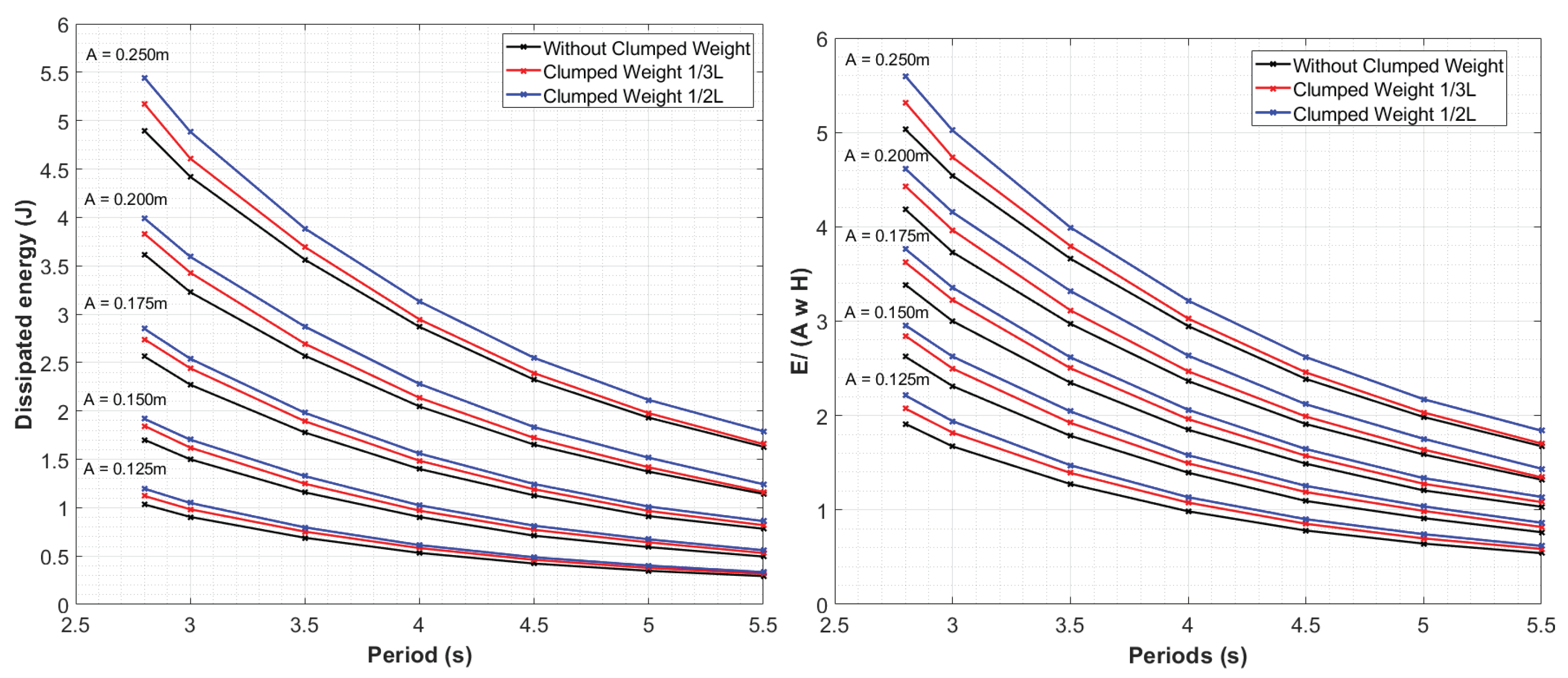
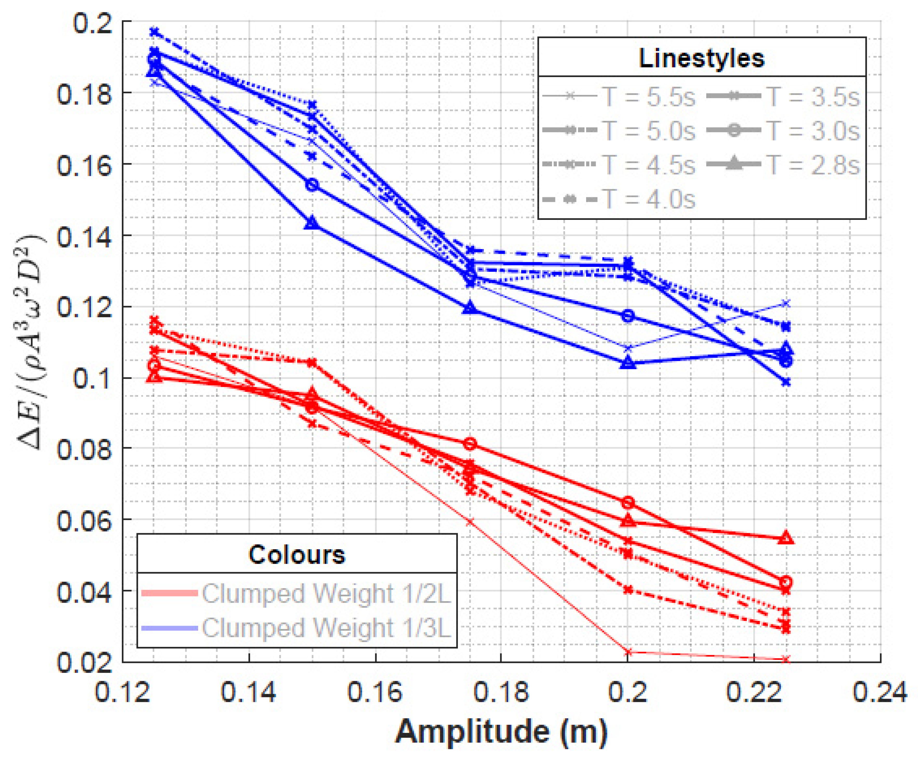
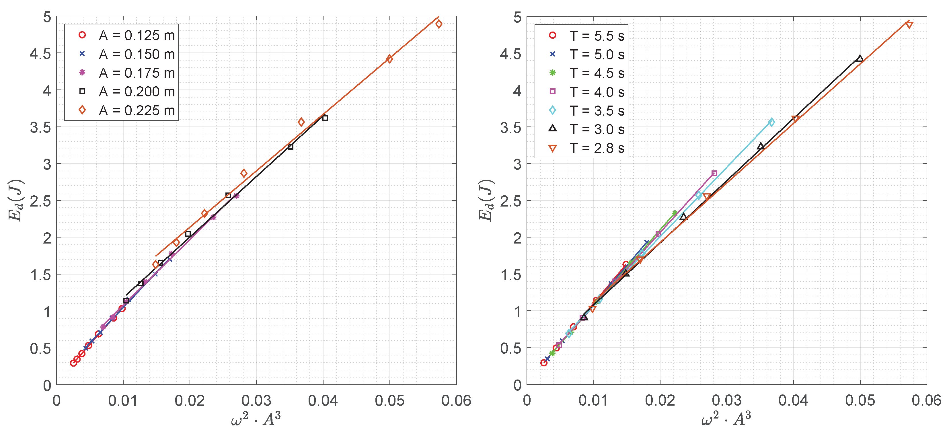
Figure 15.
Dissipated energy for all the test matrix. Dimensional form (left) and non-dimensional form (right).
Figure 15.
Dissipated energy for all the test matrix. Dimensional form (left) and non-dimensional form (right).
Figure 16.
Dissipated energy under the imposed top-end motions for the mooring line without clumped weight.
Figure 16.
Dissipated energy under the imposed top-end motions for the mooring line without clumped weight.
Figure 17.
Dimensionless increase of dissipated energy due to the Clumped weights.
Figure 17.
Dimensionless increase of dissipated energy due to the Clumped weights.
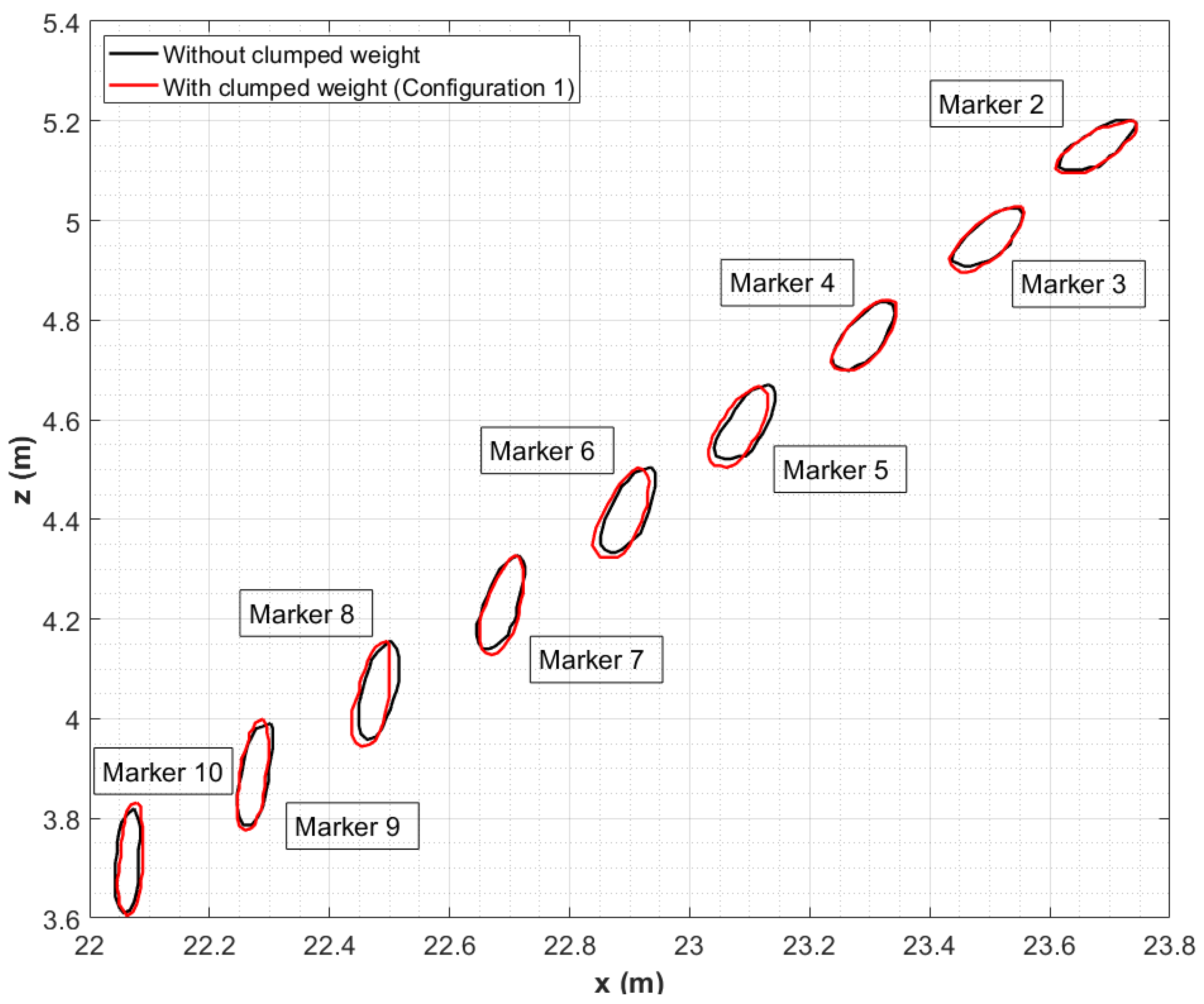
Figure 18.
Trajectories of the tracked points of the mooring line for a top-end motion of an Amplitude of m and periods s. Markers 2 to 10 are indicated in the figure.
Figure 18.
Trajectories of the tracked points of the mooring line for a top-end motion of an Amplitude of m and periods s. Markers 2 to 10 are indicated in the figure.
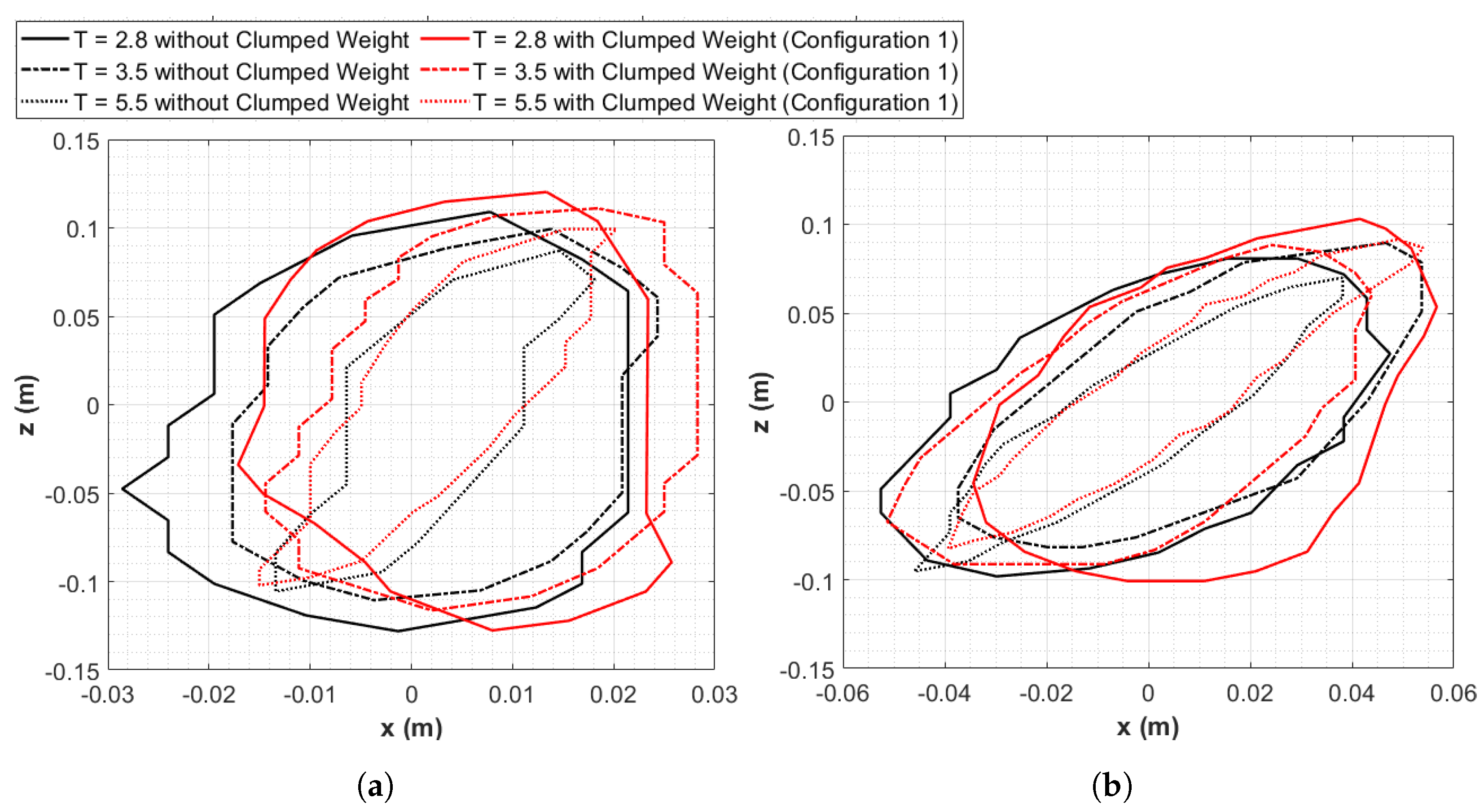
Figure 19.
Tracked motions of three points of the mooring line, for a top-end motion of an Amplitude of
m and periods
s. (
a) Trajectories of the mooring line lower point of
Figure 18 (Marker 9). (
b) Trajectories of the mooring line middle point of
Figure 18 (Marker 5). (
c) Trajectories of the mooring line upper point of
Figure 18 (Marker 2).
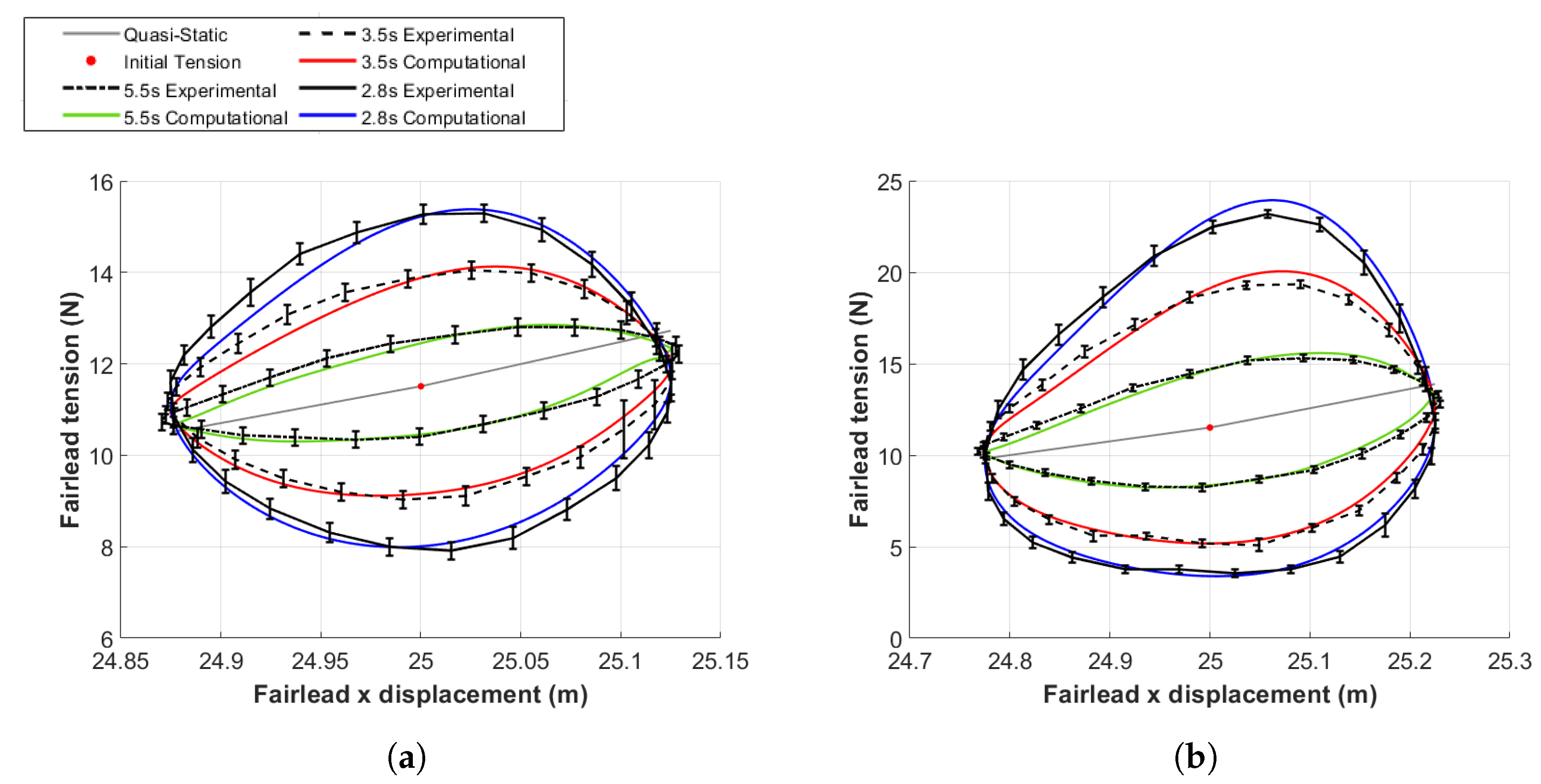
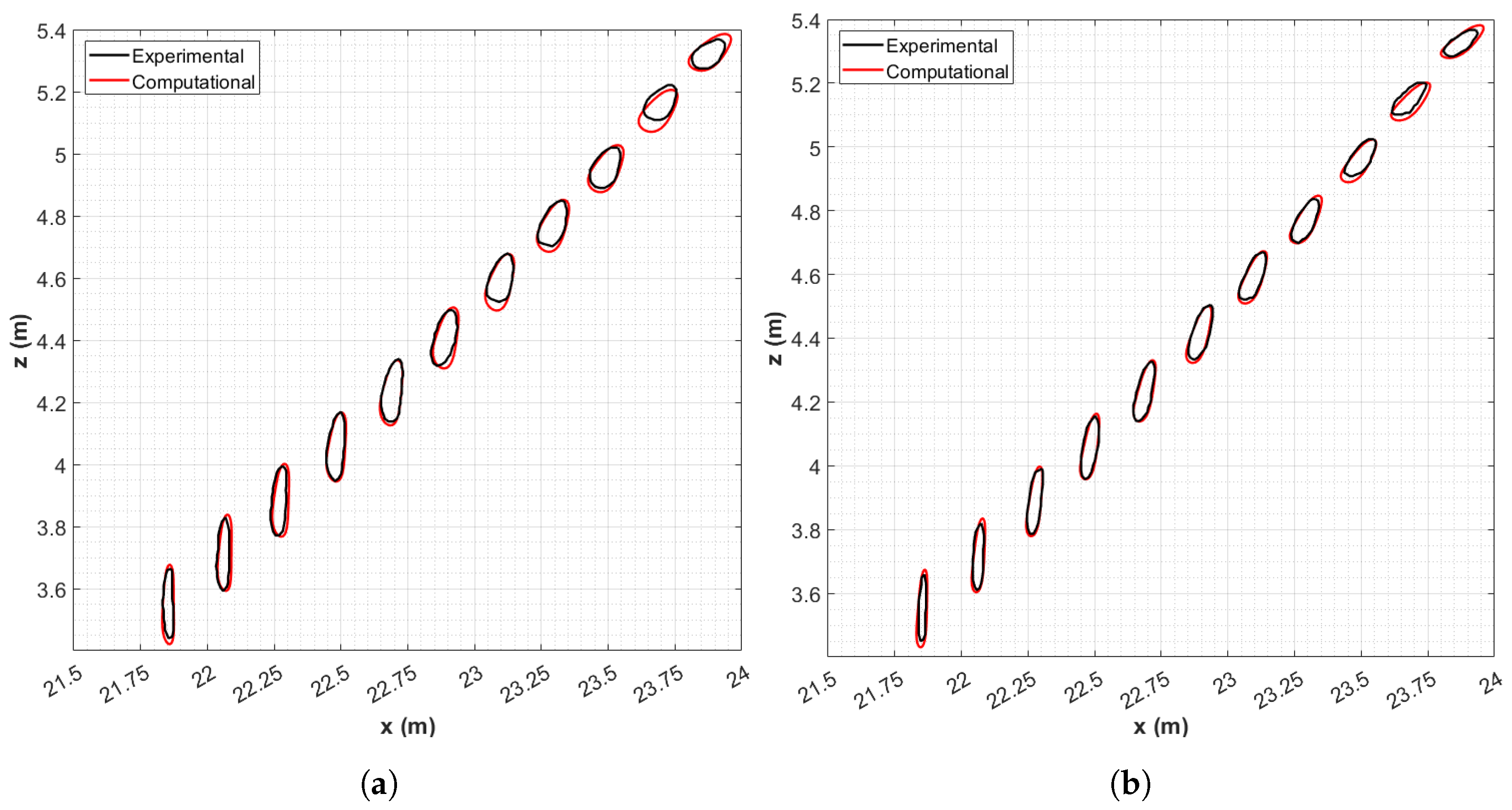
Figure 20.
Comparison between the computed fairlead tension values and the experimental measurements of the isolated mooring line for two different oscillation amplitudes m and three different periods s for the isolated mooring line. (a) m. (b) m.
Figure 20.
Comparison between the computed fairlead tension values and the experimental measurements of the isolated mooring line for two different oscillation amplitudes m and three different periods s for the isolated mooring line. (a) m. (b) m.
Figure 21.
Comparison between the computed fairlead tension values and the experimental measurements of the isolated mooring line for two different oscillation amplitudes m and two different periods s for the isolated mooring line. (a) s. (b) s.
Figure 21.
Comparison between the computed fairlead tension values and the experimental measurements of the isolated mooring line for two different oscillation amplitudes m and two different periods s for the isolated mooring line. (a) s. (b) s.
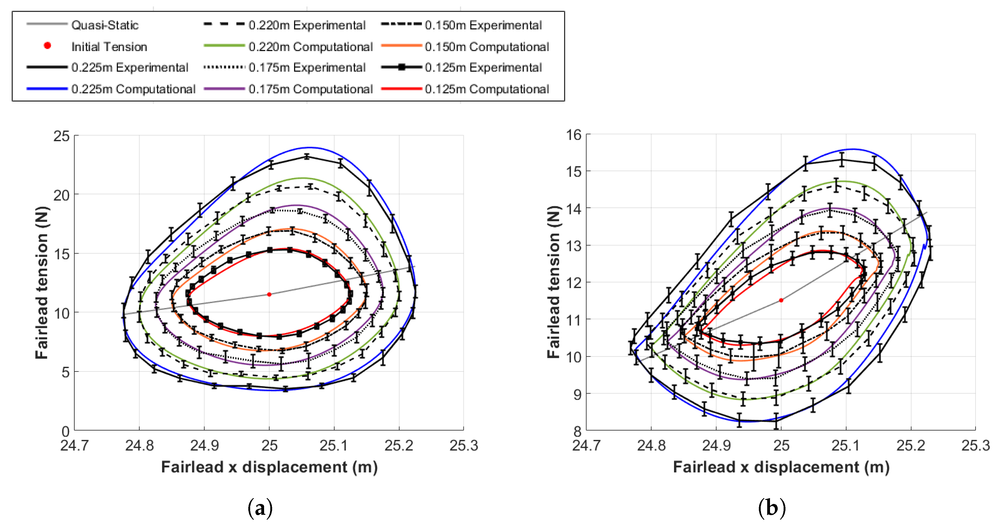
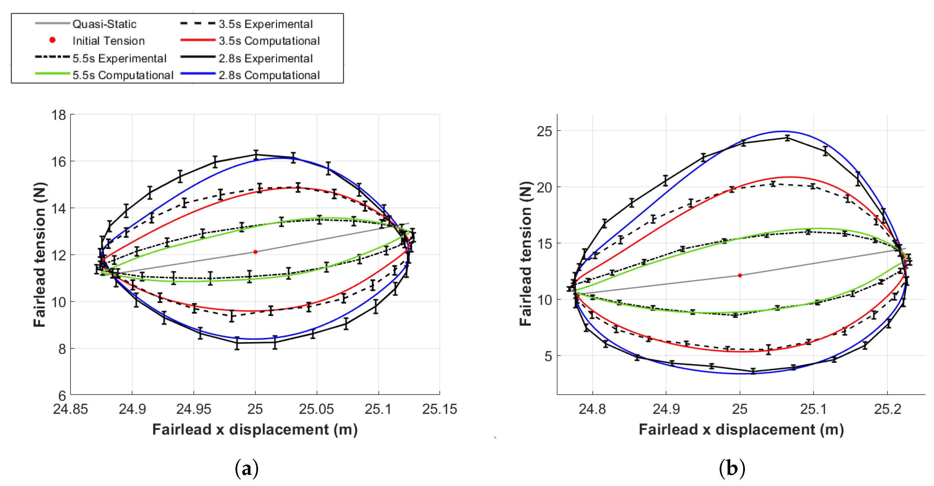
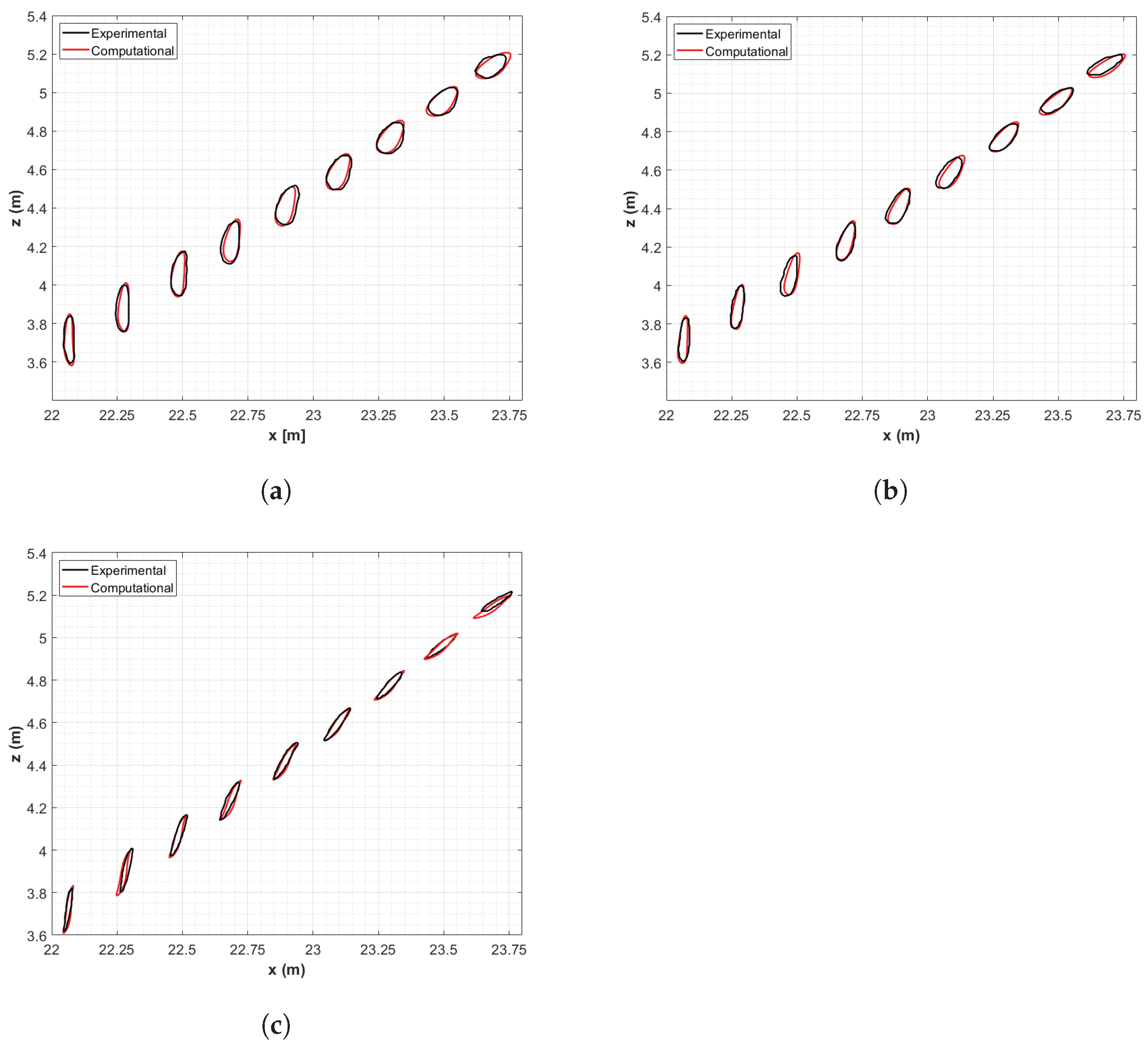
Figure 22.
Comparison between the computed fairlead tension values and the experimental measurements of the mooring line with the clumped weight in configuration 1 for two different oscillation amplitudes m and three different periods s for the isolated mooring line. (a) m. (b) m.
Figure 22.
Comparison between the computed fairlead tension values and the experimental measurements of the mooring line with the clumped weight in configuration 1 for two different oscillation amplitudes m and three different periods s for the isolated mooring line. (a) m. (b) m.
Figure 23.
Comparison between the computed fairlead tension values and the experimental measurements with clumped weight in configuration 1 for different oscillation amplitudes m and two different periods s for the isolated mooring line. (a) s. (b) s.
Figure 23.
Comparison between the computed fairlead tension values and the experimental measurements with clumped weight in configuration 1 for different oscillation amplitudes m and two different periods s for the isolated mooring line. (a) s. (b) s.
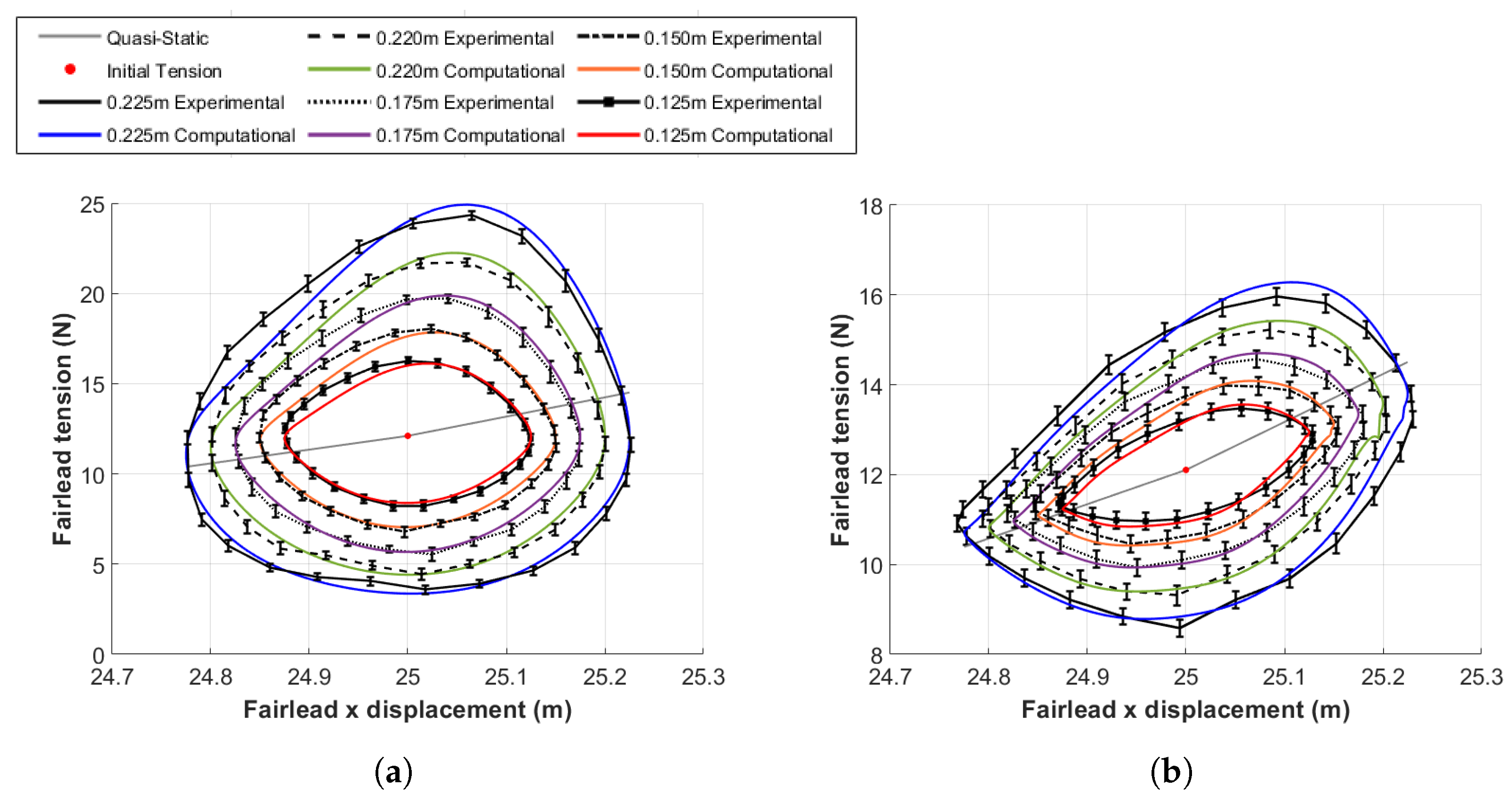
Figure 24.
Comparison between the computed fairlead tension values and the experimental measurements of the mooring line with the clumped weight in configuration 2 for two different oscillation amplitudes m and three different periods s for the isolated mooring line. (a) m. (b) m.
Figure 24.
Comparison between the computed fairlead tension values and the experimental measurements of the mooring line with the clumped weight in configuration 2 for two different oscillation amplitudes m and three different periods s for the isolated mooring line. (a) m. (b) m.
Figure 25.
Comparison between the computed fairlead tension values and the experimental measurements with clumped weight in configuration 2 for different oscillation amplitudes m and two different periods s for the isolated mooring line. (a) s. (b) s.
Figure 25.
Comparison between the computed fairlead tension values and the experimental measurements with clumped weight in configuration 2 for different oscillation amplitudes m and two different periods s for the isolated mooring line. (a) s. (b) s.
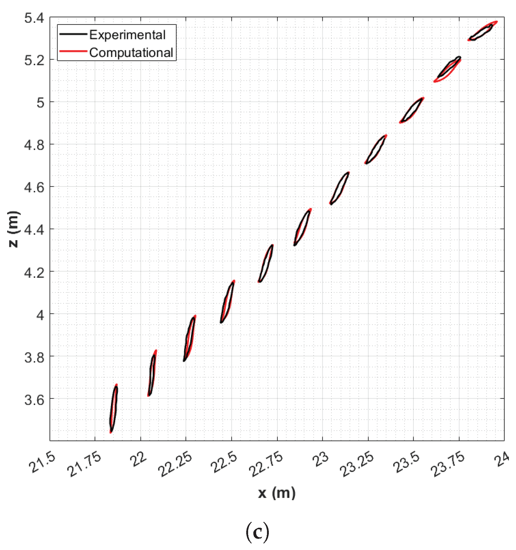
Figure 26.
Comparison between computed trajectories of catenary nodes and experimental tracked points for different oscillation periods s and amplitude m for the isolated mooring line without clumped weight. (a) s. (b) s. (c) s.
Figure 26.
Comparison between computed trajectories of catenary nodes and experimental tracked points for different oscillation periods s and amplitude m for the isolated mooring line without clumped weight. (a) s. (b) s. (c) s.
Figure 27.
Comparison between computed trajectories of catenary nodes and experimental tracked points for different oscillation periods s and amplitude m for the isolated mooring line with clumped weight (Configuration 1). (a) s. (b) s. (c) s.
Figure 27.
Comparison between computed trajectories of catenary nodes and experimental tracked points for different oscillation periods s and amplitude m for the isolated mooring line with clumped weight (Configuration 1). (a) s. (b) s. (c) s.
Table 1.
Comparison table of the existing research literature of mooring lines forced oscillations and the present work.
Table 1.
Comparison table of the existing research literature of mooring lines forced oscillations and the present work.
| | Methodology | Results | Use of Clumped Weights |
|---|
| Current work | Experimental and numerical | Dynamic analysis of tension response for different positions of clumped weights, force-displacement curves, PSD analysis, dissipated energy, trajectories, numerical validations with experiments, non-dimensional analysis. | Yes |
| Nakajima [21] | Experimental and numerical | Fairlead tension time series, frequency response curves of tension. Single frequency and amplitude with clumped weights. | Yes |
| Luo [6] | Numerical | Dynamic analysis of tension response for different positions of clumped weights. | Yes |
| Azcona [10] | Experimental and numerical | Fairlead tension, force-displacement curves, trajectories,
and numerical validation with experiments. | No |
| Li [23] | Experimental and numerical | Time series of fairlead tension, trajectories, force-displacement curve, dissipated energy, comparison of maximum fairlead tension with the static. | No |
| Barrera [9] | Experimental and numerical | Experimental fairlead tension time series comparison with numerics,
experimental time series of the displacement for different points of the line compared with numerics, sensitivity
analysis of the number of elements and computational parameters. | No |
| Bergdhal [25] | Experimental and numerical | Fairlead tension time series compared with numerics. | No |
| Yan [27] | Experimental and numerical | force-displacement curve and energy dissipation. | No |
| Barrera [7] | Experimental | Time series of fairlead tension, fairlead tension-displacement curves, trajectories, accelerations, dissipated energy, sand footprints, hydrodynamic response with different sea states | No |
| Kitney [30] | Experimental | Force-displacement curves and energy dissipation,
non-dimensional analysis. | No |
| Gao [22] | Experimental | Force-displacement curve, fairlead tension,
and PSD analysis, trajectories | No |
| Hsu [2] | Experimental | Force-displacement curve, energy dissipation and mooring line velocity vectors of image processing. | No |
| Chen [8] | Numerical | Fairlead tension time series, validation with experiments in the literature. | No |
| Qiao [24] | Numerical | Fairlead tension time series and PSD analysis, trajectories. | No |
| Webster [28] | Numerical | Force displacement curves and energy dissipation,
non-dimensional analysis. | No |
Table 2.
OC4-DeepCWind mooring system properties [
33].
Table 2.
OC4-DeepCWind mooring system properties [
33].
| | Value | Units |
|---|
| Number of mooring lines | 3 | − |
| Angle between adjacent lines | 120 | deg |
| Depth to Anchors below SWL | 200 | m |
| Depth to fairlead below SWL | 14 | m |
| Radius to Anchors from Platform Centerline | 837.6 | m |
| Radius to fairleads from Platform Centerline | 40.868 | m |
| Unstretched mooring line length | 835.5 | m |
| Mooring line diameter | 0.0766 | m |
| Equivalent mooring line mass density | 113.35 | Kg/m |
| Equivalent mooring line mass in water | 108.63 | Kg/m |
| Equivalent mooring line extensional stiffness | 753.6 | N |
| Hydrodynamic Drag coefficient for mooring lines | 1.1 | − |
| Hydrodynamic added-mass coefficient for mooring lines | 1.0 | − |
| Seabed drag coefficient for mooring lines | 1.0 | − |
| Structural damping of mooring lines | 2.0 | % |
Table 3.
Involved variables in the design of the scaled clumped weight.
Table 3.
Involved variables in the design of the scaled clumped weight.
| | Symbol | Value | Units |
|---|
| Mass | | 122.0 | g |
| Volume of displaced water | | 80.0 | cm3 |
| Diameter | | 82.3 | mm |
| Width | | 16.5 | mm |
Table 4.
Position of the red marks used for capturing the line movements.
Table 4.
Position of the red marks used for capturing the line movements.
| Marker Number | Position along the Line Measured from the Suspension Point (m) |
|---|
| 1 | 1.62 |
| 2 | 1.89 |
| 3 | 2.16 |
| 4 | 2.43 |
| 5 | 2.70 |
| 6 | 2.97 |
| 7 | 3.24 |
| 8 | 3.51 |
| 9 | 3.78 |
| 10 | 4.05 |
| 11 | 4.32 |
Table 5.
Amplitudes of the fairlead motions for .
Table 5.
Amplitudes of the fairlead motions for .
| ID | Model Scale (m) | Full Scale (m) |
|---|
| A 1 | 0.225 | 6.975 |
| A 2 | 0.200 | 6.200 |
| A 3 | 0.175 | 5.425 |
| A 4 | 0.150 | 4.650 |
| A 5 | 0.125 | 3.875 |
Table 6.
Fairlead motions periods in seconds for .
Table 6.
Fairlead motions periods in seconds for .
| ID | Model Scale | Full Scale |
|---|
| T 1 | 2.80 | 15.590 |
| T 2 | 3.00 | 16.703 |
| T 3 | 3.50 | 19.487 |
| T 4 | 4.00 | 22.271 |
| T 5 | 4.50 | 25.055 |
| T 6 | 5.00 | 27.839 |
| T 7 | 5.50 | 30.623 |
Table 7.
Parameters of the computational model.
Table 7.
Parameters of the computational model.
| | Value | Units |
|---|
| Equivalent hydrodynamic diameter (D) | 0.0033 | m |
| Unstretched Length (L) | 27.0 | m |
| Line mass density () | 7850 | Kg/m3 |
| Mass per unit length () | 0.0678 | Kg/m |
| Axial stiffness () | | N |
| Coefficient for the structural Rayleigh damping () | 0.0007 | − |
| Added mass coefficient () | 1.0 | − |
| Normal drag coefficient () | 1.445 | − |
| Tangential drag coefficient () | 0.697 | − |
| Vertical seabed stiffness () | 20.0 | N/m2 |
| Vertical seabed damping () | 0.1 | Ns/m2 |
| Tangential friction coefficient () | 0.0 | − |
| Normal friction coefficient () | 0.0 | − |
Table 8.
Maximum fairlead tension in N for all the test matrix and configurations. Notation WO CW, CW1, and CW2 denotes mooring line without clumped weight, mooring line with clumped weight (Configuration 1) and mooring line with clumped weight (Configuration 2), respectively.
Table 8.
Maximum fairlead tension in N for all the test matrix and configurations. Notation WO CW, CW1, and CW2 denotes mooring line without clumped weight, mooring line with clumped weight (Configuration 1) and mooring line with clumped weight (Configuration 2), respectively.
| Periods (s) |
|---|
| | | 2.8 | 3.0 | 3.5 | 4.0 | 4.5 | 5.0 | 5.5 | | |
| Amplitudes (m) | 0.125 | 15.35 | 14.88 | 14.07 | 13.55 | 13.2 | 12.96 | 12.80 | WO CW | Configurations |
| 16.30 | 15.78 | 14.99 | 14.31 | 13.92 | 13.65 | 13.47 | CW1 |
| 16.83 | 16.31 | 15.37 | 14.77 | 14.35 | 14.06 | 13.87 | CW2 |
| 0.150 | 16.94 | 16.32 | 15.19 | 14.45 | 13.93 | 13.57 | 13.32 | WO CW |
| 18.23 | 17.32 | 16.07 | 15.22 | 14.67 | 14.40 | 14.00 | CW1 |
| 18.44 | 17.74 | 16.56 | 15.71 | 15.13 | 15.72 | 14.42 | CW2 |
| 0.175 | 18.68 | 17.84 | 16.40 | 15.66 | 14.71 | 14.24 | 13.89 | WO CW |
| 19.86 | 18.93 | 17.29 | 16.18 | 15.44 | 14.92 | 14.54 | CW1 |
| 20.41 | 19.50 | 17.83 | 16.72 | 15.94 | 15.41 | 15.00 | CW2 |
| 0.200 | 20.73 | 19.68 | 17.80 | 16.50 | 15.63 | 15.00 | 14.55 | WO CW |
| 21.88 | 20.74 | 18.72 | 17.31 | 16.35 | 15.69 | 15.20 | CW1 |
| 22.37 | 21.33 | 19.60 | 18.12 | 17.10 | 16.28 | 15.78 | CW2 |
| 0.225 | 23.20 | 21.87 | 19.46 | 17.86 | 16.72 | 15.95 | 15.33 | WO CW |
| 24.31 | 22.83 | 20.35 | 18.59 | 17.44 | 16.58 | 15.95 | CW1 |
| 25.24 | 23.96 | 21.11 | 19.38 | 18.36 | 17.33 | 17.05 | CW2 | |
Table 9.
Minimum fairlead tension in N for all the test matrix and configurations. Notation WO CW, CW1, and CW2 denotes mooring line without clumped weight, mooring line with clumped weight (Configuration 1) and mooring line with clumped weight (Configuration 2), respectively.
Table 9.
Minimum fairlead tension in N for all the test matrix and configurations. Notation WO CW, CW1, and CW2 denotes mooring line without clumped weight, mooring line with clumped weight (Configuration 1) and mooring line with clumped weight (Configuration 2), respectively.
| Periods (s) |
|---|
| | | 2.8 | 3.0 | 3.5 | 4.0 | 4.5 | 5.0 | 5.5 | | |
| Amplitudes (m) | 0.125 | 7.826 | 8.189 | 8.959 | 9.558 | 9.876 | 10.14 | 10.34 | WO CW | Configurations |
| 7.758 | 8.247 | 9.453 | 10.04 | 10.44 | 10.64 | 10.90 | CW1 |
| 8.151 | 8.626 | 9.561 | 10.18 | 10.59 | 10.88 | 11.09 | CW2 |
| 0.150 | 6.601 | 7.116 | 8.057 | 8.693 | 9.289 | 9.662 | 9.917 | WO CW |
| 6.305 | 7.064 | 8.282 | 9.283 | 9.832 | 10.21 | 10.50 | CW1 |
| 6.941 | 7.413 | 8.55 | 9.359 | 9.874 | 10.33 | 10.63 | CW2 |
| 0.175 | 5.48 | 5.935 | 6.999 | 7.931 | 8.571 | 9.04 | 9.379 | WO CW |
| 5.56 | 6.147 | 7.036 | 8.004 | 8.914 | 9.578 | 9.995 | CW1 |
| 5.797 | 6.311 | 7.486 | 8.419 | 9.10 | 9.507 | 10.07 | CW2 |
| 0.200 | 4.388 | 4.921 | 6.074 | 6.895 | 7.779 | 8.358 | 8.805 | WO CW |
| 4.626 | 5.181 | 6.384 | 7.163 | 7.961 | 8.923 | 9.402 | CW1 |
| 4.79 | 5.40 | 6.424 | 7.467 | 8.297 | 8.911 | 9.39 | CW2 |
| 0.225 | 3.463 | 3.93 | 5.115 | 6.116 | 6.912 | 7.655 | 8.194 | WO CW |
| 3.38 | 4.222 | 5.478 | 6.496 | 7.326 | 7.881 | 8.586 | CW1 |
| 3.857 | 4.203 | 5.449 | 6.519 | 7.452 | 8.117 | 8.608 | CW2 | |


 ,
, 


