
Distribution and Environmental Impact Factors of Picophytoplankton in the Eastern Indian Ocean


Abstract
:1. Introduction
2. Methods
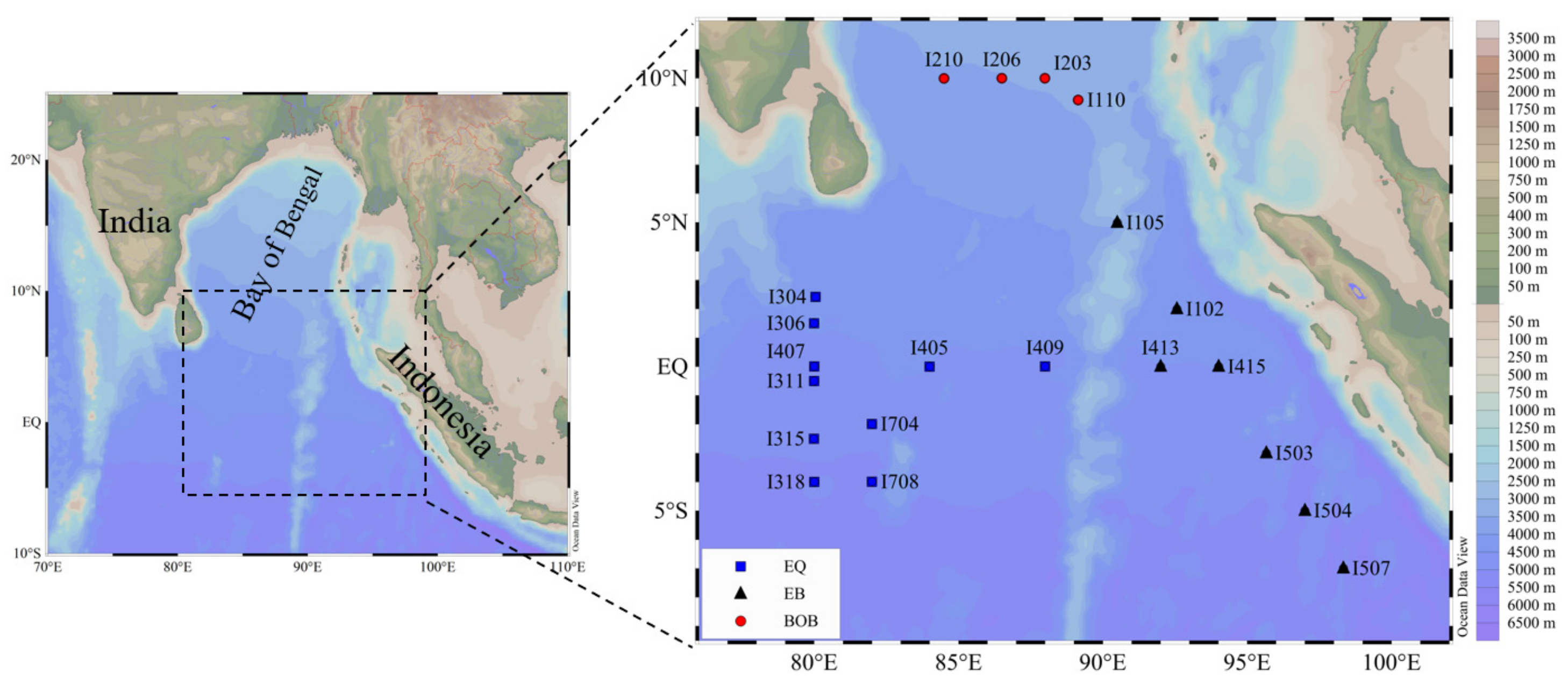
2.1. Study Area
2.2. Sampling and Analysis
2.3. Data analysis
3. Results
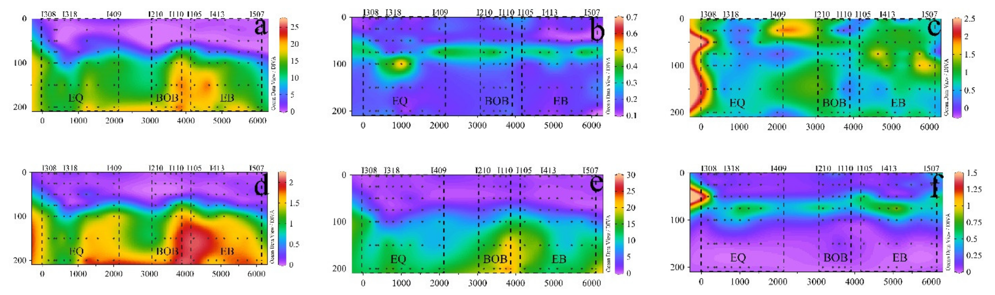
3.1. Hydrographic Conditions
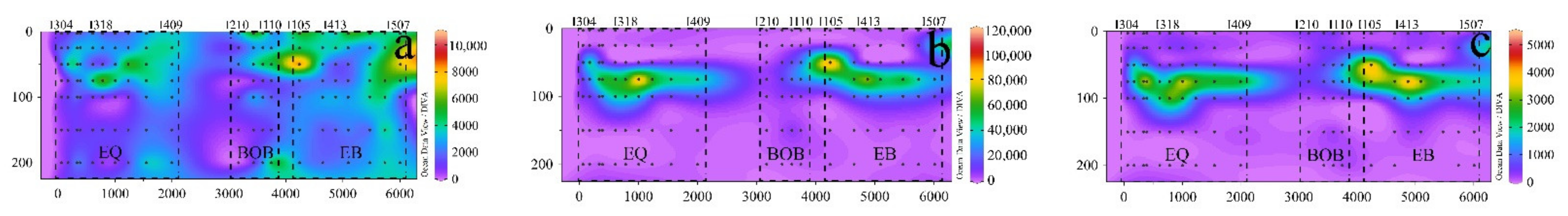
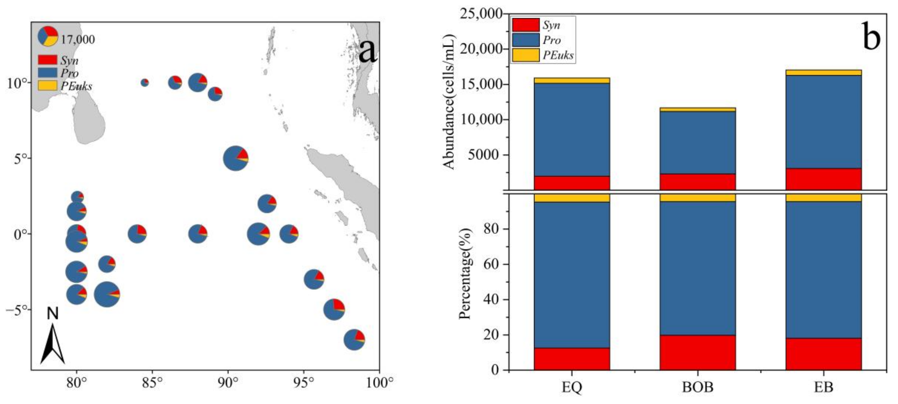
3.2. Distributions and Compositions of Pico Abundance
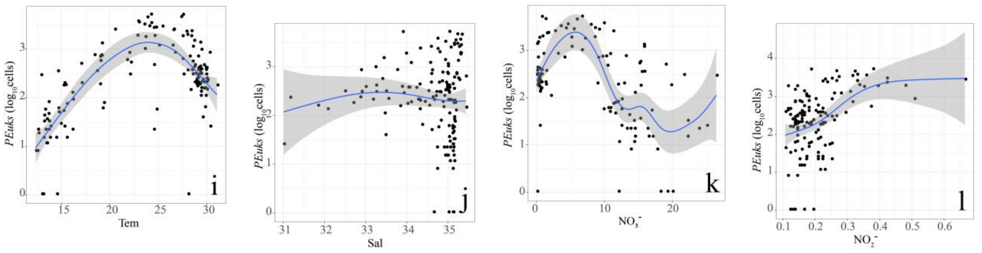
3.3. Relationship between Pico Abundance and Environmental Factors
4. Discussion
4.1. Characteristics of Pico Vertical Distribution
4.2. Coupling of Hydrography and the Pico Community
5. Conclusions
Author Contributions
Funding
Institutional Review Board Statement
Informed Consent Statement
Data Availability Statement
Acknowledgments
Conflicts of Interest
References
- Agustí, S.; Llabrés, M. Solar radiation-induced mortality of marine pico-phytoplankton in the oligotrophic ocean. Photochem. Photobiol. 2007, 83, 793–801. [Google Scholar] [CrossRef] [PubMed]
- Falkowski, P.G.; Woodhead, A.D.; Vivirito, K. Primary Productivity and Biogeochemical Cycles in the Sea; Plenum Press: New York, NY, USA, 1992; ISBN 978-1-4899-0764-6. [Google Scholar]
- Hallegraeff, G.M.; Jeffrey, S.W. Tropical phytoplankton species and pigments of continental shelf waters of north and north-west Australia. Mar. Ecol. Prog. Ser. Oldendorf 1984, 20, 59–74. Available online: http://hdl.handle.net/102.100.100/279816?index=1. [CrossRef]
- Takahashi, M.; Bienfang, P.K. Size structure of phytoplankton biomass and photosynthesis in subtropical Hawaiian waters. Mar. Biol. 1983, 76, 203–211. [Google Scholar] [CrossRef]
- Waterbury, J.B.; Watson, S.W.; Guillard, R.R.; Brand, L.E. Widespread occurrence of a unicellular, marine, planktonic, cyanobacterium. Nature 1979, 277, 293–294. [Google Scholar] [CrossRef]
- Chisholm, S.W.; Olson, R.J.; Zettler, E.R.; Goericke, R.; Waterbury, J.B.; Welschmeyer, N.A. A novel free-living prochlorophyte abundant in the oceanic euphotic zone. Nature 1988, 334, 340–343. [Google Scholar] [CrossRef]
- Li, W.; Rao, D.S.; Harrison, W.G.; Smith, J.C.; Cullen, J.J.; Irwin, B.; Platt, T. Autotrophic picoplankton in the tropical ocean. Science 1983, 219, 292–295. [Google Scholar] [CrossRef] [PubMed]
- Marie, D.; Simon, N.; Guillou, L.; Partensky, F.; Vaulot, D. Flow cytometry analysis of marine picoplankton. In Living Color; Springer: Berlin/Heidelberg, Germany, 2000; pp. 421–454. [Google Scholar] [CrossRef]
- Grébert, T.; Doré, H.; Partensky, F.; Farrant, G.K.; Boss, E.S.; Picheral, M.; Garczarek, L. Light color acclimation is a key process in the global ocean distribution of Synechococcus cyanobacteria. Proc. Natl. Acad. Sci. USA 2018, 115, E2010–E2019. [Google Scholar] [CrossRef] [Green Version]
- Zhang, Y.; Jiao, N.; Hong, N. Comparative study of picoplankton biomass and community structure in different provinces from subarctic to subtropical oceans. Deep. Sea Res. Part II Top. Stud. Oceanogr. 2008, 55, 1605–1614. [Google Scholar] [CrossRef]
- Blanchot, J.; Rodier, M. Picophytoplankton abundance and biomass in the western tropical Pacific Ocean during the 1992 El Niño year: Results from flow cytometry. Deep. Sea Res. Part I Oceanogr. Res. Pap. 1996, 43, 877–895. [Google Scholar] [CrossRef]
- Massana, R. Eukaryotic picoplankton in surface oceans. Annu. Rev. Microbiol. 2011, 65, 91–110. [Google Scholar] [CrossRef] [Green Version]
- Moon-van der Staay, S.Y.; De Wachter, R.; Vaulot, D. Oceanic 18S rDNA sequences from picoplankton reveal unsuspected eukaryotic diversity. Nature 2001, 409, 607–610. [Google Scholar] [CrossRef] [PubMed]
- Jiao, N. Marine Microbial Ecology; Science Press: Beijing, China, 2006; ISBN 7-03-018125-5. [Google Scholar]
- Fogg, G.E. Review Lecture-Picoplankton. Proc. R. Soc. Lond. Ser. B Biol. Sci. 1986, 228, 1–30. [Google Scholar] [CrossRef]
- Guo, C.; Liu, H.; Zheng, L.; Song, S.; Chen, B.; Huang, B. Seasonal and spatial patterns of picophytoplankton growth, grazing and distribution in the East China Sea. Biogeosciences 2014, 11, 1847–1862. [Google Scholar] [CrossRef] [Green Version]
- Jiao, N.; Yang, Y.; Koshikawa, H.; Watanabe, M. Influence of hydrographic conditions on picoplankton distribution in the East China Sea. Aquat. Microb. Ecol. 2002, 30, 37–48. [Google Scholar] [CrossRef] [Green Version]
- Wei, Y.; Zhang, G.; Chen, J.; Wang, J.; Ding, C.; Zhang, X.; Sun, J. Dynamic responses of picophytoplankton to physicochemical variation in the eastern Indian Ocean. Ecol. Evol. 2019, 9, 5003–5017. [Google Scholar] [CrossRef]
- Moloney, C.L.; Field, J.G. The size-based dynamics of plankton food webs. I. A simulation model of carbon and nitrogen flows. J. Plankton Res. 1991, 13, 1003–1038. [Google Scholar] [CrossRef] [Green Version]
- Yan, Z.; Tang, D. Changes in suspended sediments associated with 2004 Indian Ocean tsunami. Adv. Space Res. 2009, 43, 89–95. [Google Scholar] [CrossRef]
- Madhupratap, M.; Gauns, M.; Ramaiah, N.; Kumar, S.P.; Muraleedharan, P.M.; De Sousa, S.N.; Muraleedharan, U. Biogeochemistry of the Bay of Bengal: Physical, chemical and primary productivity characteristics of the central and western Bay of Bengal during summer monsoon 2001. Deep. Sea Res. Part II Top. Stud. Oceanogr. 2003, 50, 881–896. [Google Scholar] [CrossRef] [Green Version]
- Schott, F.A.; Xie, S.P.; McCreary Jr, J.P. Indian Ocean circulation and climate variability. Rev. Geophys. 2009, 47. [Google Scholar] [CrossRef]
- Strutton, P.G.; Coles, V.J.; Hood, R.R.; Matear, R.J.; McPhaden, M.J.; Phillips, H.E. Biogeochemical variability in the central equatorial Indian Ocean during the monsoon transition. Biogeosciences 2015, 12, 2367–2382. [Google Scholar] [CrossRef] [Green Version]
- Xuan, L.L.; Qiu, Y.; Xu, J.D.; Zeng, M.Z. Seasonal variation of surface-layer circulation in the eastern tropical Indian Ocean. J. Trop. Oceanogr. 2014, 33, 26–35. [Google Scholar] [CrossRef]
- Wiggert, J.D.; Murtugudde, R.G.; Christian, J.R. Annual ecosystem variability in the tropical Indian Ocean: Results of a coupled bio-physical ocean general circulation model. Deep. Sea Res. Part II Top. Stud. Oceanogr. 2006, 53, 644–676. [Google Scholar] [CrossRef]
- Xu, J.J.; Wang, D.X. Diagnosis of interannual and interdecadal variation in SST over Indian-Pacific Ocean and numerical simulation of their effect on Asian summer monsoon. Acta Oceanol. Sin. 2000, 22, 34–43. [Google Scholar]
- Yentsch, C.M.; Horan, P.K.; Muirhead, K.; Dortch, Q.; Haugen, E.; Legendre, L.; Zahuranec, B.J. Flow cytometry and cell sorting: A technique for analysis and sorting of aquatic particles. Limnol. Oceanogr. 1983, 28, 1275–1280. [Google Scholar] [CrossRef]
- Troussellier, M.; Courties, C.; Zettelmaier, S. Flow cytometric analysis of coastal lagoon bacterioplankton and picophytoplankton: Fixation and storage effects. Estuarine Coast. Shelf Sci. 1995, 40, 621–633. [Google Scholar] [CrossRef]
- Jiang, X.; Li, J.; Ke, Z.; Xiang, C.; Tan, Y.; Huang, L. Characteristics of picoplankton abundances during a Thalassiosira diporocyclus bloom in the Taiwan bank in late winter. Mar. Poll. Bull. 2017, 117, 66–74. [Google Scholar] [CrossRef]
- Dai, M.; Wang, L.; Guo, X.; Zhai, W.; Li, Q.; He, B.; Kao, S.J. Nitrification and inorganic nitrogen distribution in a large perturbed river/estuarine system: The Pearl River Estuary, China. Biogeosciences 2008, 5, 1227–1244. [Google Scholar] [CrossRef] [Green Version]
- Guo, S.; Feng, Y.; Wang, L.; Dai, M.; Liu, Z.; Bai, Y.; Sun, J. Seasonal variation in the phytoplankton community of a continental-shelf sea: The East China Sea. Mar. Ecol. Prog. Ser. 2014, 516, 103–126. [Google Scholar] [CrossRef] [Green Version]
- Parsons, T.R. A Manual of Chemical & Biological Methods for Seawater Analysis; Elsevier: Amsterdam, The Netherlands, 2013. [Google Scholar] [CrossRef]
- Pai, S.C.; Tsau, Y.J.; Yang, T.I. pH and buffering capacity problems involved in the determination of ammonia in saline water using the indophenol blue spectrophotometric method. Anal. Chim. Acta 2001, 434, 209–216. [Google Scholar] [CrossRef]
- Tan, J.Y.; Huang, L.M.; Tan, Y.H.; Lian, X.P.; Hu, Z.F. The influences of water-mass on phytoplankton community structure in the Luzon strait. Acta Oceanol. Sin. 2013, 35, 178–189. [Google Scholar] [CrossRef]
- Zwirglmaier, K.; Jardillier, L.; Ostrowski, M.; Mazard, S.; Garczarek, L.; Vaulot, D.; Not, F.; Massana, R.; Ulloa, O.; Scanlan, D.J. Global phylogeography of marine Synechococcus and Prochlorococcus reveals a distinct partitioning of lineages among oceanic biomes. Environ. Microbiol. 2008, 10, 147–161. [Google Scholar] [CrossRef] [PubMed]
- Graziano, L.M.; Geider, R.J.; Li, W.K.W.; Olaizola, M. Nitrogen limitation of North Atlantic phytoplankton: Analysis of physiological condition in nutrient enrichment experiments. Aquat. Microb. Ecol. 1996, 11, 53–64. [Google Scholar] [CrossRef]
- Vaulot, D.; Partensky, F. Cell cycle distributions of prochlorophytes in the North Western Mediterranean Sea. Deep Sea Res. Part A Oceanogr. Res. Pap. 1992, 39, 727–742. [Google Scholar] [CrossRef]
- Kuo, J.; Tew, K.S.; Ye, Y.X.; Cheng, J.O.; Meng, P.J.; Glover, D.C. Picoplankton dynamics and picoeukaryote diversity in a hyper-eutrophic subtropical lagoon. J. Environ. Sci. Health 2014, 49 Pt A, 116–124. [Google Scholar] [CrossRef]
- Shapiro, L.P.; Guillard, R.R.L. Physiology and ecology of the marine eukaryotic ultraplankton. Can. Bull. Fish. Aquat. Sci. 1986, 214, 371–389. [Google Scholar]
- Dela Peña, L.B.R.O.; Tejada, A.J.P.; Quijano, J.B.; Alonzo, K.H.; Gernato, E.G.; Caril, A.; Onda, D.F.L. Diversity of Marine Eukaryotic Picophytoplankton Communities with Emphasis on Mamiellophyceae in Northwestern Philippines. Philipp. J. Sci. 2021, 150, 27–42. [Google Scholar]
- Sengupta, D.; Bharath Raj, G.N.; Shenoi, S.S.C. Surface freshwater from Bay of Bengal runoff and Indonesian throughflow in the tropical Indian Ocean. Geophys. Res. Lett. 2006, 33. [Google Scholar] [CrossRef] [Green Version]
- Johnson, Z.I.; Zinser, E.R.; Coe, A.; McNulty, N.P.; Woodward, E.M.S.; Chisholm, S.W. Niche partitioning among Prochlorococcus ecotypes along ocean-scale environmental gradients. Science 2006, 311, 1737–1740. [Google Scholar] [CrossRef] [Green Version]
- Lee, Y.; Choi, J.K.; Youn, S.; Roh, S. Influence of the physical forcing of different water masses on the spatial and temporal distributions of picophytoplankton in the northern East China Sea. Cont. Shelf Res. 2014, 88, 216–227. [Google Scholar] [CrossRef]
- Liu, X.; Xiao, W.; Landry, M.R.; Chiang, K.P.; Wang, L.; Huang, B. Responses of phytoplankton communities to environmental variability in the East China Sea. Ecosystems 2016, 19, 832–849. [Google Scholar] [CrossRef]
- Chisholm, S.W.; Frankel, S.L.; Goericke, R.; Olson, R.J.; Palenik, B.; Waterbury, J.B.; Zettler, E.R. Prochlorococcus marinus nov. gen. nov. sp.: An oxyphototrophic marine prokaryote containing divinyl chlorophyll a and b. Arch. Microbiol. 1992, 157, 297–300. [Google Scholar] [CrossRef]
- Glibert, P.M.; Ray, R.T. Different patterns of growth and nitrogen uptake in two clones of marine Synechococcus spp. Mar. Biol. 1990, 107, 273–280. [Google Scholar] [CrossRef]
- Lindell, D.; Padan, E.; Post, A.F. Regulation of ntcA expression and nitrite uptake in the marine Synechococcus sp. strain WH 7803. J. Bacteriol. 1998, 180, 1878–1886. [Google Scholar] [CrossRef] [PubMed] [Green Version]
- Collier, J.L.; Brahamsha, B.; Palenik, B. The marine cyanobacterium Synechococcus sp. WH7805 requires urease (urea amiohydrolase, EC 3.5. 1.5) to utilize urea as a nitrogen source: Molecular-genetic and biochemical analysis of the enzyme. Microbiology 1999, 145, 447–459. [Google Scholar] [CrossRef] [PubMed] [Green Version]
- Glibert, P.M.; Kana, T.M.; Olson, R.J.; Kirchman, D.L.; Alberte, R.S. Clonal comparisons of growth and photosynthetic responses to nitrogen availability in marine Synechococcus spp. J. Exp. Mar. Biol. Ecol. 1986, 101, 199–208. [Google Scholar] [CrossRef]
- Wang, M.; Bai, X.G.; Liang, Y.T.; Wang, F.; Jiang, X.J.; Guo, Y.J.; Yang, F. Summer distribution of picophytoplankton in the north yellow sea. Chin. J. Plant Ecol. 2008, 32, 1184. [Google Scholar] [CrossRef]


Publisher’s Note: MDPI stays neutral with regard to jurisdictional claims in published maps and institutional affiliations. |
© 2022 by the authors. Licensee MDPI, Basel, Switzerland. This article is an open access article distributed under the terms and conditions of the Creative Commons Attribution (CC BY) license (https://creativecommons.org/licenses/by/4.0/).
Share and Cite
Wang, X.; Wang, F.; Sun, J. Distribution and Environmental Impact Factors of Picophytoplankton in the Eastern Indian Ocean. J. Mar. Sci. Eng. 2022, 10, 628. https://doi.org/10.3390/jmse10050628
Wang X, Wang F, Sun J. Distribution and Environmental Impact Factors of Picophytoplankton in the Eastern Indian Ocean. Journal of Marine Science and Engineering. 2022; 10(5):628. https://doi.org/10.3390/jmse10050628
Chicago/Turabian StyleWang, Xingzhou, Feng Wang, and Jun Sun. 2022. "Distribution and Environmental Impact Factors of Picophytoplankton in the Eastern Indian Ocean" Journal of Marine Science and Engineering 10, no. 5: 628. https://doi.org/10.3390/jmse10050628
APA StyleWang, X., Wang, F., & Sun, J. (2022). Distribution and Environmental Impact Factors of Picophytoplankton in the Eastern Indian Ocean. Journal of Marine Science and Engineering, 10(5), 628. https://doi.org/10.3390/jmse10050628