Different Types of Near-Inertial Internal Waves Observed by Lander in the Intermediate-Deep Layers of the South China Sea and Their Generation Mechanisms

Abstract

We report the direct and quantitative measurement of five significant near-inertial waves (NIWs) events observed by Lander at water depths of 600 m to 1100 m at 119°17′ E and 22°06′ N in the northern South China Sea from July to November 2017. We found that these five NIWs events lead to strong shearing, which plays an important role in deep water mixing. Each event corresponds to several different NIWs generation mechanisms. The results show that the NIWs events generated by typhoons were the most regular. This was caused by dispersive NIWs propagation over long periods of time and over long distances. NIWs formed by spontaneous generation do not have this feature. The strongest NIWs events during the observation period were caused by a combination of shelf wave attenuation and monsoon. This time, the signal was transmitted to the seabed, and the upward signal reflected in the meridional direction was found. The reflected signal was anisotropically affected by the seabed topography. A horizontally propagated NIWs event with relatively weak dispersion was also found in this study. Based on the topography, we suspect it was formed by the Lee wave, but we cannot provide any more useful evidence.

1. Introduction

Near-inertial waves (NIWs) are common components in the internal wave field of the ocean. It can be identified by spectral analysis, showing a prominent peak in the frequency band close to the local inertial frequency (f = 2Ωsinφ, where Ω and φ denote the angular velocity of the earth’s rotation and latitude, respectively) [1,2]. Unlike internal tidal waves, NIWs have more pronounced propagation characteristics and vertical structures [2]. As a necessary process of energy transfer from large scale to small scale, NIW events have been the focus of research in recent years [2,3]. NIWs can produce large vertical shears to induce energy dissipation in the horizontal direction, resulting in ocean mixing, which in turn can affect biogeochemistry and climate [4,5,6].

The NIWs are subject to multiple generation mechanisms, and thus are featured by different propagation characteristics. In general, the generation mechanisms of NIWs can be classified as wind forcing at the sea surface [7,8,9], parametric subharmonic instability (PSI) and wave–wave interactions [10,11], Lee waves formation by geostrophic flow over the seafloor [12,13] and spontaneous generation [14]. Sea surface wind forcing is considered as the main generation mechanism of NIWs [2]. The NIWs have been widely observed after tropical cyclones or hurricanes. Once the NIW is initiated, it radiates downward into the stratified interior, draining energy from the mixed layer and ultimately depositing it in the form of turbulent mixing, which acts as a sink for near-inertial energy [2,15].

The South China Sea (SCS) is vulnerable to tropical cyclones with an average of approximately 18 typhoons passing by per year. Consequently, the NIWs have been well captured by in situ observations in the SCS. Based on three years’ mooring data, Chen et al. suggested that the NIWs signal show highest intensity in August, September and October [16]. Further investigation shows that the energy of the NIW is associated with the strength of the typhoon. For example, the corresponding near-inertial kinetic energy (NIKE) would increase by 18%, 38% and 19%, if the radius of maximum wind speed, maximum wind speed, or moving velocity of typhoon was increased by 10%, respectively [17]. In addition, abrupt changes in sea surface wind induced by summer monsoon onset also could trigger NIWs [18]. When the energy is transmitted to a depth of more than 500 m, the wind-induced NIWs events gradually weaken [19]. Therefore, in waters deeper than 500 m, the NIWs induced by other factors are expected to be stronger than those induced by sea surface wind. Meanwhile, the generation mechanisms of the NIWs also tend to be dominate by other factors rather than by the sea surface wind below 500 m water depth. The spontaneous generation is one of the main reasons for the NIWs in deep layers with water depth greater than 500 m. After the local rotation balance structure is destroyed by subinertial current, the NIWs could be generated because of the Rossby adjustment [20]. The mechanisms fall into two categories: frontogenesis [21], in which NIWs arise as instabilities in a sharpening front formed by large-scale strain, and radiation by time-dependent instabilities of the low-frequency flow [14]. The earliest research on the generation of NIWs from the front began with atmospheric fronts [22,23]. Later, Danioux et al. [24] used a 2 km resolution primitive equation ocean model to show that gravity waves are emitted from large-Rossby-number flow associated with density filaments near the surface. Shakespeare and Taylor [25] discovered that a two-dimensional front with frontal action can radiate inertial gravity waves. The researchers found that localized wave packets are emitted when thin filaments in the surface density are formed by straining, leading to large vertical vorticity and correspondingly large Rossby numbers. Nagai et al. [26] observed strong NIWs shear in the Kuroshio front, which means that the spontaneous generation of NIWs represents a redistribution of quasi-geostrophic energy rather than a significant sink.

It is difficult to analyze NIWs with different generation mechanisms at the same location, which requires the availability of data in complex seas and multiple NIWs confirmation methods. For the South China Sea, the characteristics of complex seas are not difficult. The South China Sea is the marginal sea of the Northwest Pacific, with an average depth of 1212 m and a maximum depth of 5559 m. The complex topography and frequent typhoon passages lead to various generation mechanisms of NIWs have been studied in the South China Sea. In the South China Sea, NIWs energy and shear are significantly enhanced and exceed tidal counterparts by a factor of 2 to 3 in the upper layer during typhoons [27]. Guan et al. [7] found that the NIWs generated by Typhoon Megi interacted with the D1 tidal component, damping the generation of NIWs. Due to the existence of the Luzon Strait in the northeastern part of the South China Sea, vertical heaving by strong internal tides can Doppler shift NIWs to frequencies higher than f in the Eulerian spectra [3], causing the South China Sea to have strong wind fields but no long-term or deep NIWs. The formation of NIWs in the South China Sea can be caused by factors other than wind. Xie et al. [11] found that even at noncritical latitudes in the South China Sea, NIWs signals are generated by the PSI mechanism. Hu [13] also found that NIWs pulses are generated when the South China Sea seabed eddy passes by, and these NIWs events are generated by the lee wave mechanism. Since different NIWs have different generation mechanisms, the NIWs events generated by different mechanisms must also have different characteristics. The comparison of NIWs with different formation mechanisms in the South China Sea lacks sufficient research. Sun et al. [28] compared the NIWs characteristics generated by three typhoons and verified that the negative vorticity strengthens the NIWs phenomenon. Cao et al. [29] compared five NIWs events and found two NIWs events that were not caused by typhoons. Those two NIWs had larger wavenumbers and smaller wavelengths and produced stronger shear in deep water.

Previous studies have investigated different types of NIWs in the SCS. However, most of these studies focus on the upper layer. Meanwhile, these NIWs are generally case studies that occurred in different locations. On 25 July 2017, we have deployed a Lander equipped with an upward looking Acoustic Doppler Current Profiler (ADCP) to observe the current velocity profile in the northwest of the Luzon Strait. A total of 124 days continuous time series was obtained. The observation has captured 5 NIWs with different generation mechanism at the same location, which has not been reported yet. In this study, the features and generation mechanisms of the pronounced 5 NIWs are investigated and compared. This paper is organized as follows. Section 2 introduces the data and methods. Section 3 represents the observed features of the NIWs. Section 4 analyzed the generation mechanisms of the different NIWs. Discussion is given in Section 5, and it is followed by the summary.

2. Data and Methods

2.1. Lander Observation

During the summer and fall of 2017, the research Lander was moored at 1135 m water depth in the northwestern of the Luzon Strait (119°17′ E, 22°06′ N) (Figure 1a). The Lander was equipped with an upward looking 75 kHz ADCP to measure the current velocity covering the water depth of approximately 600–1100 m, with vertical resolution of 8 m and time interval of 20 min. A total of 124 days continuous time series (from 25 July to 25 November) were collected. Figure 1b shows a diagram of Lander and its instrumentation. During the Lander observation period, there are 5 typhoons, namely, the Guchol, Mawar, Hato, Haitang, and Roke, which may be related to the 5 NIWs, passed by the SCS and are marked in Figure 1a.

2.2. Sea Level Anomalies

Sea surface height anomalies are provided by the French National Space Research Center Satellite Oceanography Archive Data Center (AVISO official website) and shared on the website (https://resources.marine.copernicus.eu/?option=com_csw&task=results, accessed on 27 June 2018). AVISO integrates and differentiates a number of different satellites, such as Seasat-A, ERS-1, TOPEX/POSEIDON, Jason-1, and Envisat-1, to form a global grid of data and greatly improves the observational data spatial and temporal resolutions. With the advancement of technology in ocean data collection, the current data within a range of tens of kilometers from the shore are all credible.

2.3. Cross-Calibrated Multiplatform Wind Vector Analysis

The wind field data are a marine wind field product developed by the Physical Oceanography Distributed Active Archive Center (PO. DAAC) of the National Aeronautics and Space Administration (NASA), shared on the website (https://climatedataguide.ucar.edu/climate-data/ccmp-cross-calibrated-multi-platform-wind-vector-analysis, accessed on 3 July 2018). The Cross-Calibrated Multi-Platform (CCMP) wind analysis is a near-global raster dataset with high spatial and temporal resolutions, covering surface wind vectors from 1987 to present. The input data are a combination of mutually calibrated satellite data from numerous radiometers and scatterometers and in situ data from moored buoys. The algorithm uses ERA-Interim to reanalyze the wind as a first guess and finds the best solution for all available observations.

2.4. Accurate Algorithm for Frequency and Phase

For the data whose sampling frequency is Fs, the frequency at a certain n point obtained by spectral analysis is

$$Fn=(n-1)\cdot Fs/N$$

(1)

where N is the total number of samples. It can be seen from the above formula that the frequency that Fn can distinguish is Fs/N. For ADCP data, the time interval was 20 min and the average time of analysis per event was 12 days. This means that Fs is 72 d⁻¹ and N is 864. Several values around the inertial band (f₀ = 0.752 cpd) are 0.667 cpd (0.886 f₀), 0.750 cpd (0.997 f₀) and 0.833 cpd (1.11 f₀). A more precise frequency distribution is not available. Since the frequency and phase determined by spectrum analysis are not adequately accurate, we can observe the frequency and phase of NIWs by fitting the function to an equation [30,31].

$$V(t)=v_0+v_1\sin (2\pi f_{i}t+\theta )+R(t)$$

(2)

where V(t) is the time series, v₀, v₁, f_i and θ are the parameters to be fitted, and R(t) is the residual.

NIWs are a type of inertial gravity wave. For inertial gravity waves propagating freely in the ocean, the velocity satisfies the following equation:

$$\begin{array}{l}U=u\cos (kx+ly+mz-\omega t)\\ V=v\sin (kx+ly+mz-\omega t)\end{array}$$

(3)

where k, l, and m are the wavenumbers of the waves. ω is the angular velocity for the NIW, and ω = 2πf. For the Lander observation data, both x and y are constants. Thus, Equation (3) can be simplified as follows:

$$\begin{array}{l}{U}_{NIW}=u\cos (mz-2\pi ft+{\theta }_0)=u\sin (mz-2\pi ft+{\theta }_0+\frac{\pi }{2})\\ V_{NIW}=v\sin (mz-2\pi ft+{\theta }_0)\end{array}$$

(4)

According to a comparison between the results of Equations (2) and (4), θ has a linear relationship with depth.

$$\theta =mz+{\theta }_0$$

(5)

At the same time, the downwardly propagating NIWs correspond to m < 0, so the deeper the water depth is, the greater the m value is. Conversely, if m does not change or decrease with water depth, the NIWs events propagate horizontally or upward. Moreover, Equation (4) shows that the phase difference between the zonal (U) and meridional (V) directions is 90 degrees for the same NIWs under ideal conditions.

In short, there are three advantages to using this method of analysis. First of all, the accurate peak frequency and wave number can be obtained by this method. Secondly, the composition of the signal can be analyzed by the phase difference. Finally, the vertical wave number can be obtained from the slope of the phase.

2.5. Bicoherence

Many waves that comprise the internal wave field of the ocean are not independent because they interact with each other. Bicoherence [32] determines the specific frequency and wavenumber of the interaction. Here, we will give a very brief overview of the bicoherence method. We define the frequency bispectrum over the Fourier frequency pair (ω₁, ω₂) as follows:

$$B({\omega }_1,{\omega }_2)=E[X_k{X}_l{X}_{k+l}^{*}]$$

(6)

where $X_{k+l}^{*}$ is the complex conjugate of $[X_{-(k+l)}]$ and E[] is the expected value. The size of the bispectrum depends on the size and relative phase of each Fourier coefficient. If the volatility is the sum of statistically independent stochastic oscillators, the bispectrum will be zero. However, if some oscillations are caused by nonlinear coupling between other oscillations, nonzero values will be produced. Therefore, the bispectrum is a measure of the dependence within the wave triad (ω_k, ω_l, ω_k+l).

The bispectrum can be normalized to eliminate the influence of wave amplitude, resulting in bicoherence b(k,l), which is defined as follows:

$$b^2(k,l)=\frac{{\left|B(k,l)\right|}^2}{E[{\left|X_k{X}_l\right|}^2]E[{\left|X_{k+l}^{}\right|}^2]}$$

(7)

When the bicoherence of the sample exceeds zero by an appropriate threshold, it is shown to be statistically significant, where thresholds for the 90%, 95%, and 99% confidence levels at m degrees of freedom (dof) are respectively given as follows:

$$b_{80\%}=\sqrt{3.2/m},b_{90\%}=\sqrt{4.6/m},b_{95\%}=\sqrt{6/m}$$

The number of degrees of freedom is two times the independent realizations. As mentioned above, if the three components of a triad are independently applied so that the linear combination of their phases is zero, a significant bicoherence value may appear.

3. Results

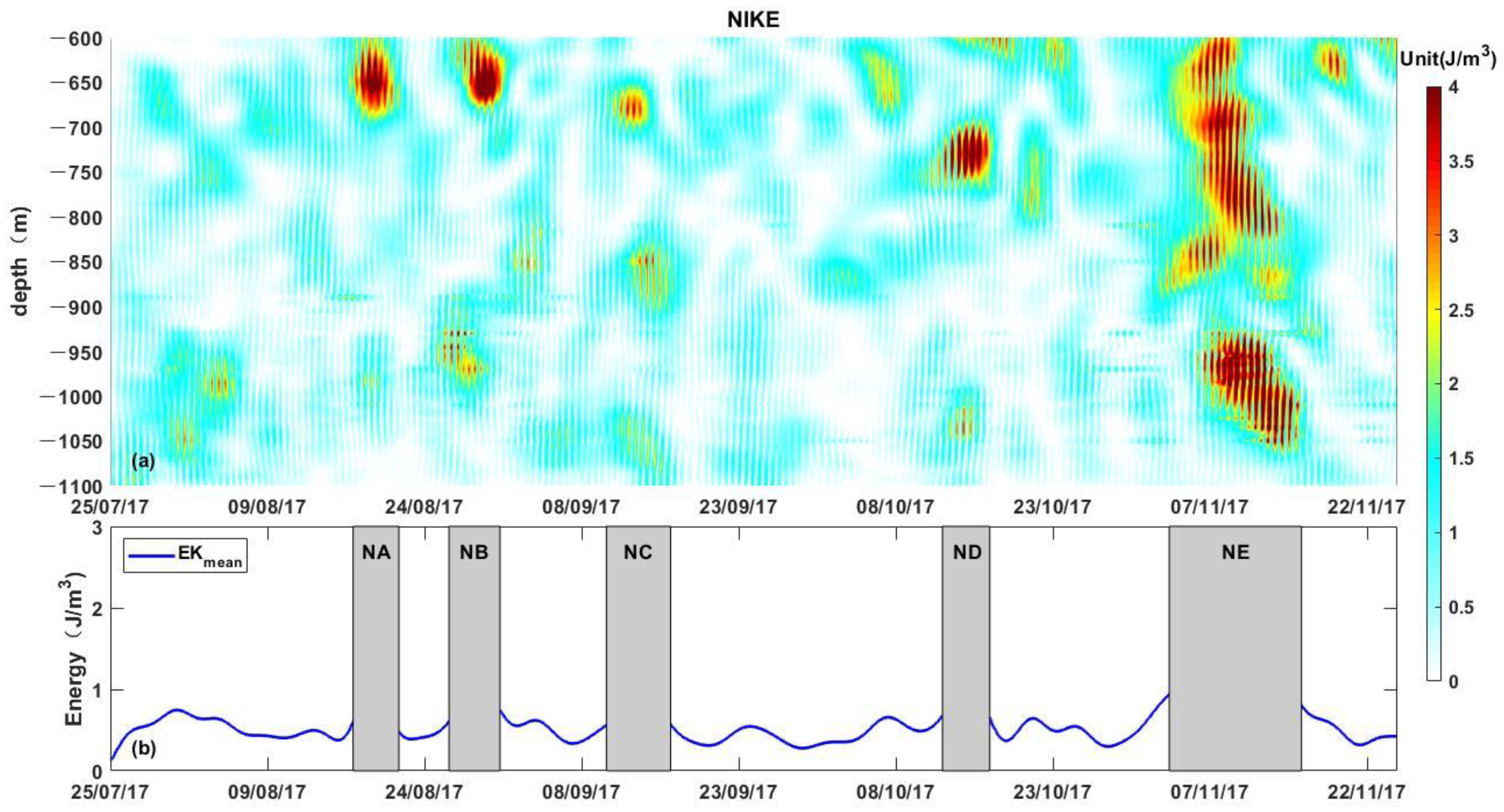
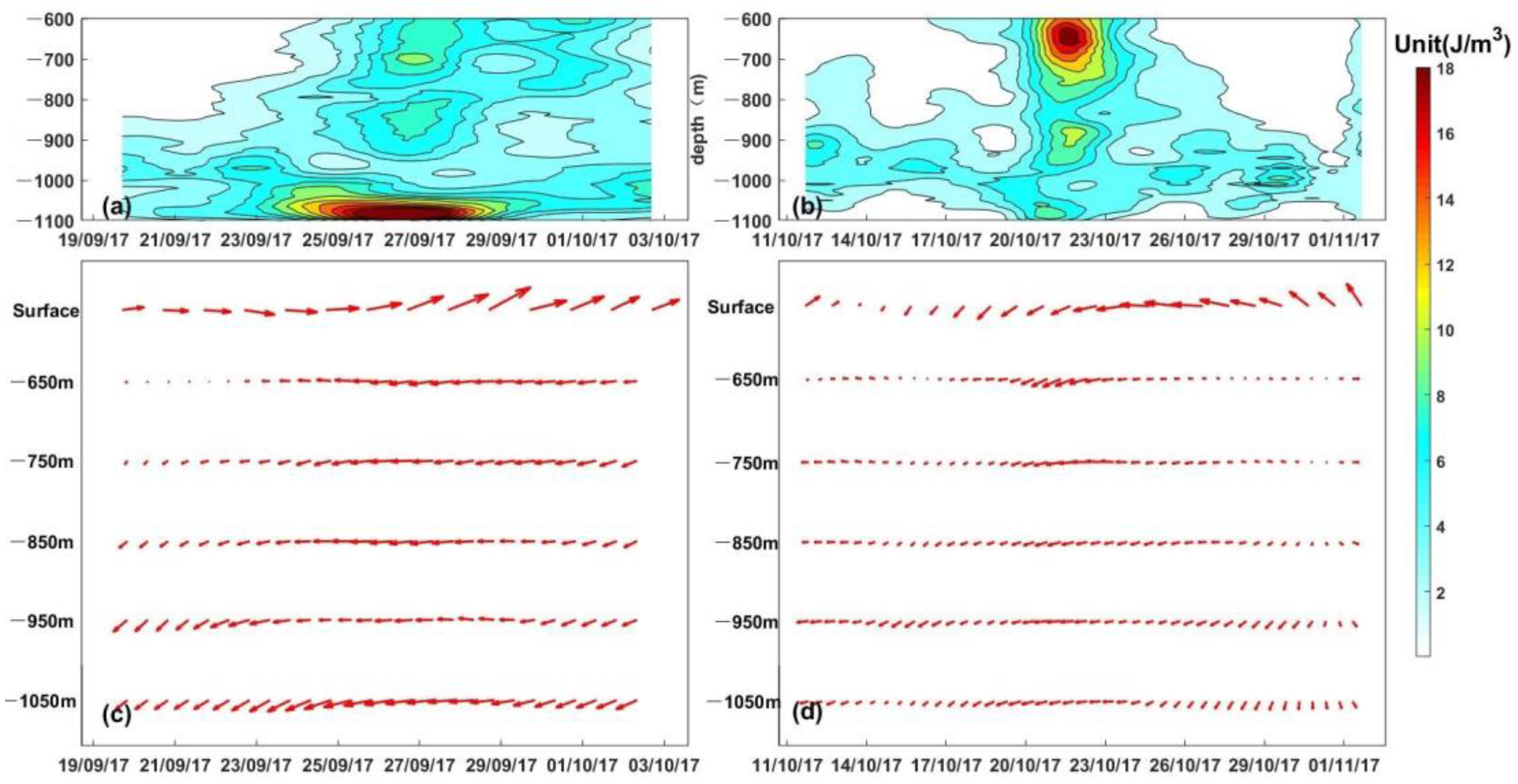
3.1. Spatiotemporal Distribution of Near-Inertial Kinetic Energy

To analyze NIWs characteristics, we filter the flow velocity collected by ADCP. The bandpass range is from 0.8 f₀ to 1.2 f₀. Figure 2 shows the velocity profile of the filtering results. Similar to many previous observational studies, NIKE had obvious discontinuities—e.g., [16]. The results can show five distinct NIWs events. Here, NIWs events A, B, C, D, and E (NA, NB, NC, ND, and NE, respectively) are used to name these five phenomena. The reason why the five obvious NIWs events were selected was because their corresponding maxima were more than one standard deviation range of the average NIKE. The depth distribution of NIKE, NIKE = 0.5ρ(u_f² + v_f²) (J/m³), shown in Figure 3a, shows the temporal and spatial distributions of NIKE during the Lander observations. Figure 3b shows the depth average of NIKE. The main NIKE during the observation period is marked by the shaded part of Figure 3b. The apparent NIWs time period was determined using the following method. Firstly, the time of maximum value of the depth-averaged NIKE was found. Then, the nearest minimum on both sides of the maximum was found. Finally, the time midpoint between the maximum value and the minimum value was considered to be the starting point and ending point of a significant NIWs period. For example, the first maximum value of NA kinetic energy appeared on 19 August, and the corresponding minimum values on both sides were 15 August and 23 August. We selected the NA time period as 17 August to 21 August. The same method was used to determine the NIWs events of NB, NC, ND, and NE.

As shown in Figure 2, the meridional direction of the near-inertial velocity was significantly higher than the zonal direction. This was due to the elliptical polarization of the observed NIWs events. Although these five events all produced NIKE enhancements, their apparent distribution locations vary vertically. In the NA, NB, and NE events, the strongest flow velocity occurred in the uppermost layer of the observations. This was most likely the energy passed down from above. At the same time, in the NE event, NIKE had a strong velocity in the whole water depth. This was very abnormal, indicating that the formation mechanism of this event may not be a single condition. This study will analyze the mechanism by which these events occurred.

Observing the NIKE in the intermediate-deep layer during these 124 days (Figure 3), energy signals with different characteristics were discovered. At some point, the main strong NIKE area was close to the shallowest water of the observation range, such as NA and NB. Occasionally, the main strong NIKE area appeared at deeper water depths, such as NC and ND. Additionally, the main strong NIKE area appeared in the entire observation water depth area, such as NE, throughout the observed water depth. The appearance of different NIKE characteristics showed that the NIWs generation mechanism were different in the observed time interval.

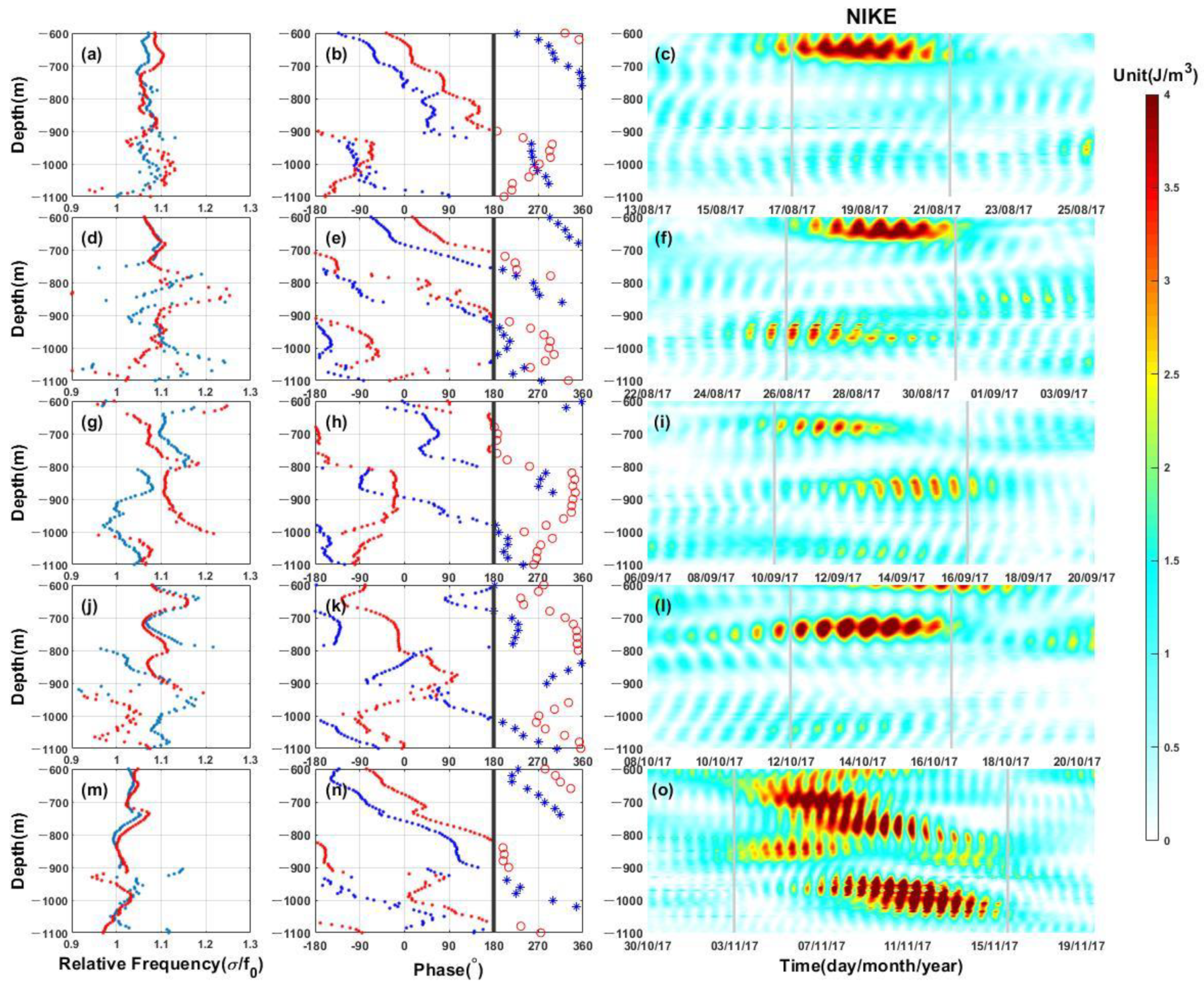
3.2. Frequency and Phase of Five NIWs

Since NIWs are transmitted upward or downward, there will be a ‘skew’ in the time distribution of velocity. Of the five events, it is clear that NA and NB are more skewed, and ND appears to be less skewed. These inclinations are related to the vertical wavenumber, so next, we will use the method in Section 2 to find the frequency, phase, vertical wave-number and other characteristics of several NIWs events.

The composition of NIWs events can be analyzed by observing the change in the vertical wavenumber. Each NIWs event will generate signals with a wide frequency range, among which high-mode signals are easier to dissipate and low-mode signals are easier to transmit over a long distance. This leads to different NIWs events with different characteristics after long time and long-distance propagation. Although the NIWs events transfer energy to other frequencies through PSI, its own frequency will not change drastically with propagation. If a significant change in wavenumber or frequency was observed at a certain depth, the NIWs events deeper than this depth and the NIWs events shallower than this depth was not the same signal. Using this method, the frequency and phase of five obvious NIWs events were calculated, and the characteristics of five obvious NIWs events were analyzed.

The strongest NIKE of NA occurred in the shallowest position (600–700 m) of the observation area (Figure 4c). By studying the NIWs event in this water depth range, the depth of influence at this part of the NIWs event is found. In the phase depth distribution map (Figure 4b), the NIWs phase basically showed a relatively stable linear change in part of the water depth below 800 m, and the phase became larger with water depth, which indicated that the vertical wavenumber m < 0. Therefore, the main signal of NA actually affects depths of 600 m to 800 m. The frequency of this event was 1.08 f₀. Through function fitting, the vertical wavenumber is −0.013 m⁻¹. Figure 4a shows that the NIWs frequency of this depth range was concentrated at approximately 1.08 f. NA in the deep-water area was different from the NA at shallower than 800 m depth. Firstly, the phase was basically unchanged along the water depth, which shows that the vertical wavenumber was basically close to zero, and the NA signal in the deep-water area propagates weakly downward. Secondly, the frequency variation along the water depth is much greater in the deep-water area.

NB and NA had similarities in the water depth distribution of NIKE, and the strongest NIKE also occurred in the shallowest position (600–685 m) (Figure 4f). A strong difference was a NIKE spike in deep water (925–975 m). The same analytical method that was used for NA was also used for NB. Although the downward wave signal extends in the shallowest position (Figure 4e), the signal in the shallowest position and a signal in middle water (685–925 m) had different characteristics and were not the same signal. By fitting the slopes, we know that the vertical wavenumber in shallow water was −0.015 m⁻¹. The frequencies in the zonal and meridional directions were same, and the frequency was about 1.09 f₀. In deep water depth, the vertical wavenumber was stable at −0.035 m⁻¹, and the vertical wavenumber was different from that in the shallowest position. The frequencies in the zonal and meridional directions are no longer consistent. The phase and frequency of the NIWs event in deep water became chaotic, and there was no stable frequency or phase (Figure 4d,e). The NIWs event in deep water again became regular. From the NIKE point of view, this part corresponds to energy intensities in deep water. The occurrence of this signal is slightly earlier than that of shallow water. The signals in the zonal and meridional directions were different. The vertical wavenumber in the zonal direction was −0.008 m⁻¹, and the vertical wavenumber in the meridional direction was −0.020 m⁻¹. In summary, the shallow NIWs affects water depths from 600 m to 685 m. The deep NIWs influence water depth ranged from 925 to 975 m. The NIWs of the two parts were not the same NIWs events.

The NIKE of NC had three peaks along the different water depths (Figure 4i). This study of NC was divided into three parts: upper, middle, and lower. The common feature of the three parts was that the signals in the zonal and meridional directions did not have the same frequency, and the phase difference between these two directions was not 90 degrees (Figure 4h). Unlike NB and NA, the largest NIKE of NC did not occur in the shallowest position of the observations. The strongest NIKE was located in the water depth range of 640 m to 700 m. The frequency in the zonal direction was 1.1 f₀, and the frequency in the meridional direction was 1.08 f₀. The frequency in the zonal direction was greater than the frequency in the meridional direction (Figure 4g). The vertical wavenumbers in the zonal direction and the meridional direction were different (0.009 m⁻¹ and 0.006 m⁻¹). The frequency in the meridional direction changed sharply. This reason was sufficient to conclude that the signals in the zonal and meridional directions were not the same signal. The water depth of the middle part of NC ranged from 810 m to 950 m. The signal in the meridional direction was stable. The frequency was 1.1 f₀, and the phase did not change with depth. This result shows that the vertical wavenumber in the meridional direction was zero. The zonal direction signal was chaotic, and it is impossible to find a pattern. The lower part was at the bottom of the NC, which was 1050 m deeper. The frequency and phase were relatively stable. The frequency varied with depth around approximately 1.06 f₀. The phase change with depth was also relatively small.

The ND had only one maximum energy value in the depth distribution, so we focused on the NIWs event in this water depth range (700–790 m) (Figure 4l). The phase analysis shows that the phase of this depth did not change with water depth. This finding showed that the vertical wavenumber of the NIWs event at this water depth was zero (Figure 4k). Energy did not propagate downward. At the same time, we also found that the frequencies of the water depth in the zonal and meridional directions were basically the same, and both increased with water depth. The average frequency was 1.09 f₀. (Figure 4j). The frequency also changed with depth in the same trend, and the phase difference between these two directions was larger than 90°. This result would cause ND to produce an elliptical polarization. In general, the frequency and phase of the strongest ND NIKE zone were the same, but the frequency was not fixed along the water depth. The phase difference between the zonal and meridional directions was not 90°. The phase difference did not change with the depth of the water, but the frequencies in both directions vary uniformly with water depth. Therefore, the reason for the generation of ND was different from the previous one.

NIKE of NE could be observed across the whole water depth (Figure 4o). Detailed analysis revealed that the signals were still different. In the shallowest position (600–720 m), the frequencies in the zonal and meridional directions were maintained at 1.03 f₀ (Figure 4m). The phase difference between the two directions was basically maintained at 90° (Figure 4n). The vertical wavenumber was estimated to be −0.017 m⁻¹. Then, the zonal and meridional direction signals changed from 740 m to 820 m. There was a difference in frequency, and the frequency was not the same as the uppermost layer in the two directions. The phase difference between the two directions was also less than 90°. The vertical wavenumber was −0.026 m⁻¹. However, this phenomenon only lasted until 820 m, and then, from depths of 820 m to 880 m, the phase difference between the zonal and meridional directions changed back to 90°. Another feature of this part of the NIWs event was that the vertical wavenumber was equal to zero, and the energy did not propagate downward with depth. The frequency was equal to f₀, which was lower than the frequency of all NIWs events observed over the entire 124 days. This part of the low-frequency NIWs could be found in NIKE, corresponding to the NIKE near a water depth of 850 m before November 8th. As the water depth reached 940 m, a NIKE peak was found. Then, through the frequency distribution, the zonal and meridional direction signals of this NIWs no longer showed the same changing trend. The NIWs event in the zonal direction ranged from 940 m to 1050 m. The phase increased with water depth, the energy propagated downward, and the vertical wavenumber was approximately −0.028 m⁻¹. The meridional direction was divided into two sections at 985 m, and the vertical wavenumber of the signal from 940 m to 985 m was 0.020 m⁻¹. This result corresponds to the upward of energy, which was not seen during the entire observation period. The NIWs vertical wavenumber in the meridional direction below 985 m was −0.038 m⁻¹, and the corresponding energy continued to propagate downward. To summarize the characteristics of NE, there was a clear dividing line at 880 m. The vertical wavenumbers of the zonal and meridional directions of the NE at water depths shallower than 880 m were constantly changing and could be divided into three types of NIWs event: two downward signals and one horizontally propagating signal. The wavenumbers in the zonal and meridional directions of the signal at water depths shallower than 880 m were not the same, and an upward-propagating NIKE was observed.

In general, during the NC period, the NIWs event showed a significant difference between the zonal and meridional directions. Analyzing the two events of NA and NB, we know that the zonal and meridional directions of the strongest NIKE had a phase difference of 90 degrees. However, this phenomenon was not found in the three parts of NC. When analyzing NB, we found that there was another energy peak in the area with the largest NIKE depth, and they had a phase difference that was not 90 degrees. This signal period occurred slightly earlier than the main signal of NB. Therefore, the mechanism of the NC was different from the NB.

Based on analysis, the five NIWs events we determined have different characteristics. To summarize, the events were divided into the following situations. The NIWs event were sometimes downward (NA, NB, and NE) and sometimes not (NC and ND). The phase difference between the zonal and meridional directions was sometimes 90 degrees (NA, NB, and NE) and sometimes not 90 degrees (NC and ND). The frequency did not always change with water depth (NA and NB), but it occasionally changed with water depth (NC, ND, and NE). These different characteristics of NIWs events mean that each event had a different generation mechanism. Here, we analyze the formation mechanism of these NIWs through a series of analyses and explain the NIWs phenomenon under different mechanisms. In Section 4, the mechanism of different NIKE characteristics is analyzed through different ocean and atmospheric characteristics.

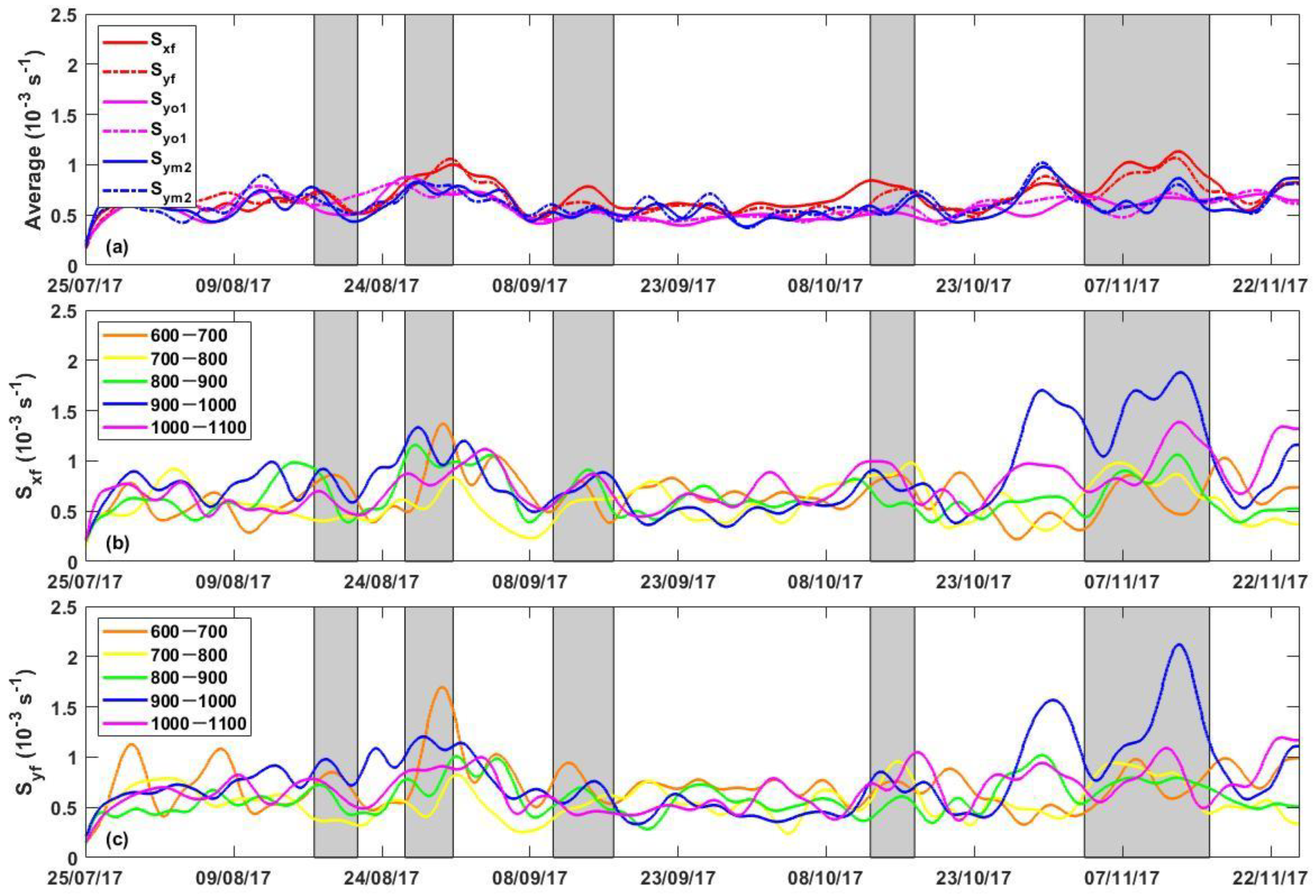
3.3. Shearing of Near-Inertial Waves

Although the NIWs events were not as strong as the surface layer, the position of the NIWs events in the energy cascade in the deep-water area cannot be ignored. This section would discuss the role of mid-deep NIWs in shearing and energy cascades in the South China Sea.

The characteristics of NIWs under different generation mechanisms were analyzed above. Now, we compare the effects of different NIWs on mixing. Figure 5a shows the vertical shear of the NIWs velocity averaged across the water depth. First, the shear of NIWs was stronger than the shear of the semidiurnal tide and diurnal tide during the observation period. The NIWs shear was stronger than the baroclinic tidal shear on the overall time average, which shows that although the NIWs in the South China Sea occurred intermittently [2] and were not easily transmitted below 500 m [3], the mixed contribution of NIWs at depths of 600 m to 1100 m was still stronger than the semidiurnal tide and the full diurnal tide. Second, the NIWs shear in the zonal direction was slightly higher than that in the meridional direction. This result showed that in the deep-water environment, due to the influence of terrain and other environmental factors, the elliptical characteristics of the near-inertial current were more obvious.

As is shown in Figure 5b,c, under different NIWs events, the strongest shearing of NIWs also occurs at different water depths. The strongest shearing of NA and NB occurred at the shallowest water depth tested, that is, at depths of 600 m to 700 m. At the same time, the shearing was also very strong at depths of 900 m to 1000 m. During ND, the strongest energy occurred at a water depth of 700 to 800 m, but from the perspective of shearing, the shearing at this water depth was less than the bottom mixing at 1000 to 1100 m. The strongest shearing during NE also occurred at water depths of 900 m to 1000 m. This water depth range was exactly the same as the water depth range of the energy upward signal. Therefore, the mixing enhancement from 900 m to 1000 m water depth was largely dependent on the reflection of NIKE from the seabed. In general, NA and NB had strong mixing at depths of 600 to 700 m. However, the water depth corresponding to the overall strongest mixing occurs at water depths of 900 to 1000 m.

4. NIWs Generation Mechanism

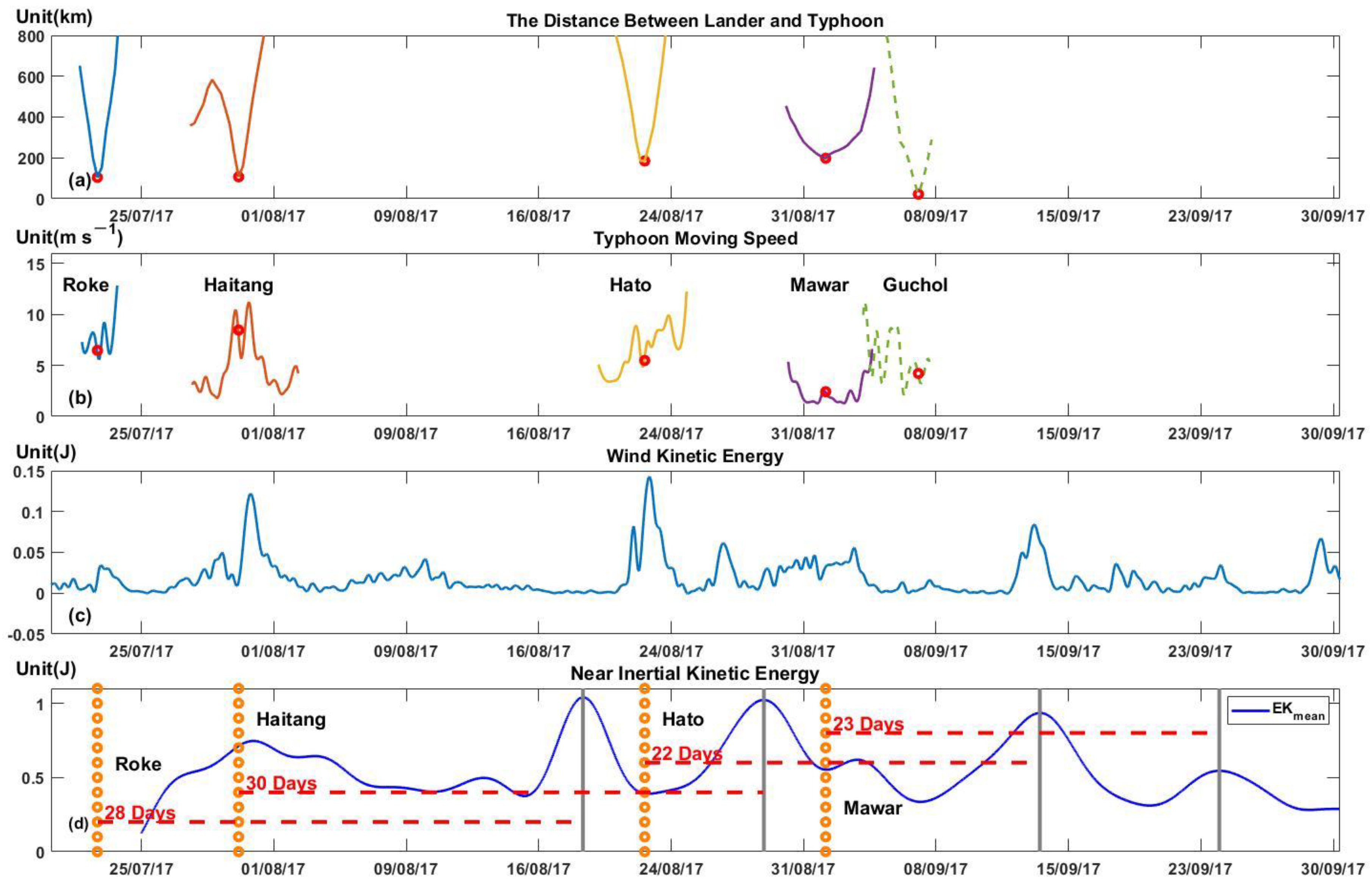
4.1. Typhoons

Typhoons are the main formation mechanism of NIWs in the South China Sea. Therefore, the characteristics of typhoons are very important for understanding the NIWs events observed by Lander. Previous studies have shown that a strong NIWs event will form after a typhoon, e.g., [33]. However, due to the strong nonlinear interaction of the currents in the South China Sea, the NIWs events decay rapidly, and it is difficult to pass below 500 m, e.g., [28]. Whether the NIWs events generated by the typhoon can be observed within the range of 600 m to 1100 m remains to be confirmed. Taking these into account, the typhoon characteristics during the observation period are shown in Figure 6. With the typhoon data of the Japan Meteorological Agency, the typhoon’s distance from the Lander and the movement speed of the typhoon are shown in Figure 6a,b, respectively. The time at which each typhoon was closest to the Lander is marked with a red circle for each typhoon phenomenon in the three pictures. The wind kinetic energy at the Lander location is also plotted in Figure 6c using CCMP data. The NIKE from 18 July to 1 October is also shown in Figure 6d. To discover the relationship between NIKE and typhoons, we marked the typhoon on NIKE. At the same time, the time difference between the maximum value of NIKE and the closest typhoon is shown.

By comparing the typhoon information with NIKE (Figure 6d), the typhoon characteristics from 20 July to 15 September and the NIWs events from 10 August to 30 September show good corresponding characteristics. Five typhoon events were discovered during the observation period. The specific characteristics of these five typhoons are shown in

Table 1. Characteristics of the five typhoons when they were closest to Lander.

Typhoon	Closest Distance (km)	Moving Speed (m/s)	Central Pressure (hPa)	Closest Time	NIW	Energy Maximum Time	Time Difference (Days)
Roke	104.27	6.46	1004	22 July	NA	19 August	28
Haitang	107.15	8.46	985	30 July	NB	29 August	30
Hato	184.82	5.48	975	22 August	NC	13 September	22
Mawar	198.09	2.41	996	1 September	Weak NIWs after NC	24 September	23
Guchol	2.63	4.20	1006	7 September			17

. During the NIWs period from 10 August to 30 September, there were three obvious, strong NIWs events, namely, NA, NB, and NC. After NC, there was a weaker NIWs energy bump. Four NIWs correspond to these five typhoons. Whether all NIWs were affected by the typhoon requires further investigation.

Typhoons Roke, Haitang, Hato, Mawar, and Guchol and their corresponding NIWs lag by 28 days, 30 days, 22 days, 23 days, and 17 days, respectively (Table 1). The fourth and fifth typhoons corresponded to weak NIWs events behind NC. According to the conclusion of Xu et al. [17], when the three parameters (radius of maximum wind speed, maximum wind speed, and moving velocity of typhoon) increase by 10%, the corresponding NIKE increases by 18%, 38%, and 19%, respectively. The maximum wind speed has the greatest impact on NIW. Therefore, Typhoons Roke and Haitang were more likely to produce strong NIWs. Typhoons Hato and Mawar traveled further distances at slower moving speeds. The maximum wind speed of Typhoon Guchol was low, and its moving speed was very slow. If all four NIWs events were caused by typhoons, a weaker NIWs event was transmitted to deep water faster, which was obviously impossible. Therefore, some NIWs events were not generated by typhoons.

According to the feature analysis of NIWs, the main signal regions of NA and NB had similar features. These two NIWs had several common features. Firstly, the vertical wavenumber was less than zero, which shows that the NIWs were downward energy transmission. These characteristics were similar to the NIWs generated by typhoons observed by previous study, e.g., [30,31]. Secondly, the observed frequency and wavenumber were relatively regular in the upper level of observations, and they were more chaotic in the lower level. In other words, the NIWs observed in the upper layer generally had a phase difference of 90° in the zonal and meridional directions, and the estimated vertical wavenumbers and frequencies in the zonal and meridional directions were the same. The phase difference between the zonal and meridional directions in the chaotic state of the lower layer was not 90 degrees. At the same time, the frequencies of the NIWs in the upper zonal and meridional directions were not the same, and they were not fixed values. The signal is the same as the near-inertial signal generated by the typhoon in previous study [34]. Thus, the upper NIWs event was the NIWs event generated under the influence of the typhoon. This signal was generated in the mixed layer and then passed down. This occurrence was why the observed vertical wavenumbers were all less than zero. This signal had regular characteristics. The zonal and meridional directions had the same frequency and wavenumber, and the phase difference between the zonal and meridional directions was also 90°. Observing NB in the deep-water area was not directly caused by the typhoon. The characteristic of this part of the signal was the signal anisotropy, the zonal and meridional direction signals had different wavenumbers, unfixed frequencies and a phase difference that was not 90°. These features were also found in NC and the weak NIWs event behind NC. Next, this study reveals why typhoon-generated NIWs have these characteristics.

According to previous research, a typhoon would produce NIWs events, a high-modal signal that quickly dissipates locally. The other was a low-mode signal, which was easier to transmit over a long distance [2]. Therefore, the signals transmitted to a distant location must have the same characteristics. In other words, the main signals of NA and NB 700 were generated from the mixed layer and transmitted down to the deep-water area. Using Figure 4a–i to analyze the impact depth of the NIW, Typhoon Roke caused the deepest NA impact. The second greatest impact was NB caused by Typhoon Haitang. In contrast, NC was very unlike the NIWs triggered by a typhoon. Although the weak NIWs event behind NC and NC could correspond to several typhoon events, the two evets had no obvious downward characteristics, no obvious 90-degree phase difference, and the largest NIKE did not occur. These two NIWs events (NC and the weak NIWs event behind NC) were different from previous NIWs event observations on typhoon generation [32,33]. Meanwhile, NA and NB were the NIWs events triggered by typhoons, which could be demonstrated by another method. If it was assumed that the depth of the mixed layer was 50 m and the NIWs were generated one day after the typhoon, the vertical group velocities of NA and NB were 20 m d⁻¹ and 19 m d⁻¹, respectively. This result was combined with the estimated vertical group velocity by NIKE data (18 m d⁻¹ and 17 m d⁻¹), which was basically consistent.

Based on Figure 6 and Table 1, the three factors most closely related to the NIKE are the distance the typhoon passes through Lander, the wind speed, and wind kinetic energy when it passes. Among the three typhoons, Typhoon Roke was the closest to Lander, and Typhoon Haitang and Typhoon Roke were approximately the same distance from Lander. Typhoon Hato and Typhoon Mawar were nearly at twice the distance from the previous two typhoons. Although both Typhoon Haitang and Typhoon Hato could generate strong wind kinetic energy at Lander’s location, as Haitang was closer, the generated NIWs event was stronger, which was why the impact of NB was stronger than NC. As Typhoon Mawar was too far away from Lander, it did not generate significant wind kinetic energy in the Lander position. The central air pressure of Typhoon Guchol was too high, the generated wind kinetic energy was too weak, and the wind kinetic energy could not be seen from the Lander position. Combining several NIWs characteristics, we find that when the wind kinetic energy was greater than 0.04 J, the transmission depth of the NIWs generated by typhoons were only related to the distance of the typhoon from Lander. When the typhoon was too far away, even if the wind kinetic energy at the observation location was strong, NIWs cannot be transmitted down to a water depth below 600 m.

Based on the above inferences, Typhoons Roke and Haitang generated NIWs events in the mixed layer and passed to the observation waters to form NA and NB. We found that these two NIWs had several common features. Firstly, the vertical wavenumber was less than zero, showing that the NIWs generated by a typhoon will have downward energy transmission. Secondly, the observed frequency and wavenumber were relatively regular in the upper level of the observations, and they were more chaotic in the lower level. In other words, the NIWs observed in the upper layer generally had a phase difference of 90° in the zonal and meridional directions, and the estimated vertical wavenumbers and frequencies in the zonal and meridional directions were the same. The phase difference between the zonal and meridional directions in the chaotic state of the lower layer was not 90 degrees. At the same time, the frequencies of the NIWs in the zonal and meridional directions were not the same, and they were not fixed values. Thus, a conclusion can be obtained that the upper NIWs event was the NIWs event generated under the influence of the typhoon. This signal was generated in the mixed layer and then passed down, which was why the observed vertical wavenumbers were all less than zero. As the NIWs event was dispersive, the signal had regular characteristics after travelling over long distances. The zonal and meridional directions had the same frequency and wavenumber, and the phase difference between the zonal and meridional directions was also 90°. Observing the lower NIWs event was not directly caused by the NIWs event generated by the typhoon. NC was not an NIWs event generated by a typhoon in the mixed layer.

4.2. Role of the Parametric Subharmonic Instability Mechanism

The PSI mechanism, as one of the main excitation mechanisms of NIWs, should be discussed. Higher-order spectral analysis, such as bicoherence (normalized bispectrum), can be used to distinguish between nonlinearly coupled waves and waves that have been independently excited [30,35,36]. The NIWs event generated by the PSI mechanism in the South China Sea did not necessarily occur at critical latitudes [11]. At the same time, Boyer et al. [3] found that the South China Sea was prone to nonlinear interactions, which made it difficult to generate strong NIWs events in the South China Sea. Cao et al. [28] investigated whether NIWs were triggered by internal tides by calculating the correlation between an NIWs and M2 tides, NIWs and M2 + f, and NIWs and M2 − f. If the NIWs events had strong correlation with the internal tide signal, the NIWs events were generated by internal tides through PSI. If the correlation was weak, these two signals were generated by different mechanisms and then interacted.

As mentioned above, the two NIWs of NA and NB were caused by typhoons, so we focused on the three events of NC, ND, and NE. Figure 7 presents the average of the bicoherence of the velocities in the zonal and meridional directions from all depth bins between 600 and 1100 m. However, no obvious PSI phenomenon occurred in these three events. Especially during the NE event, we found that the NIWs events had a strong correlation with the M2 tide signal and the M2 − f signal (not shown in this study), but the result of the bicoherence value was very weak, indicating that each event was not a PSI effect.

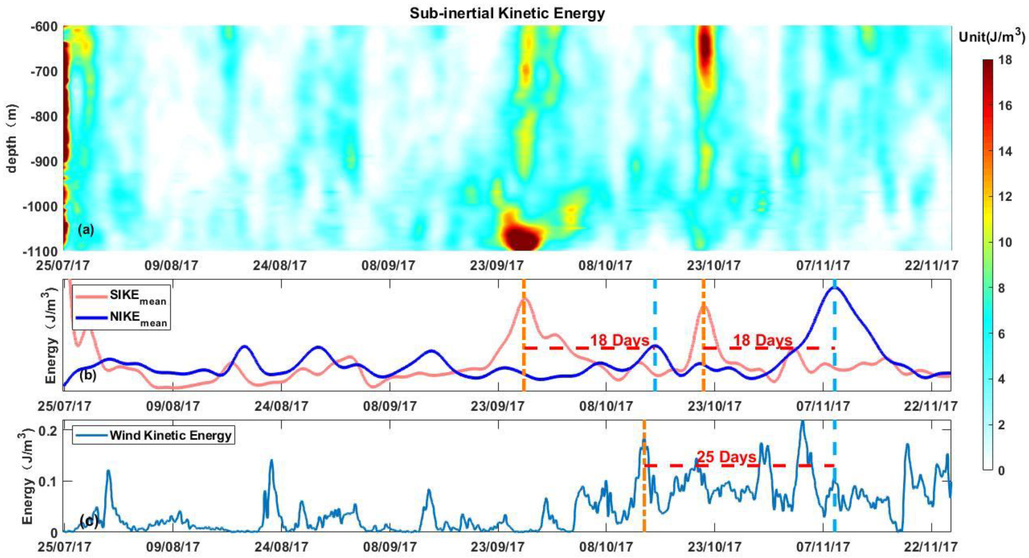
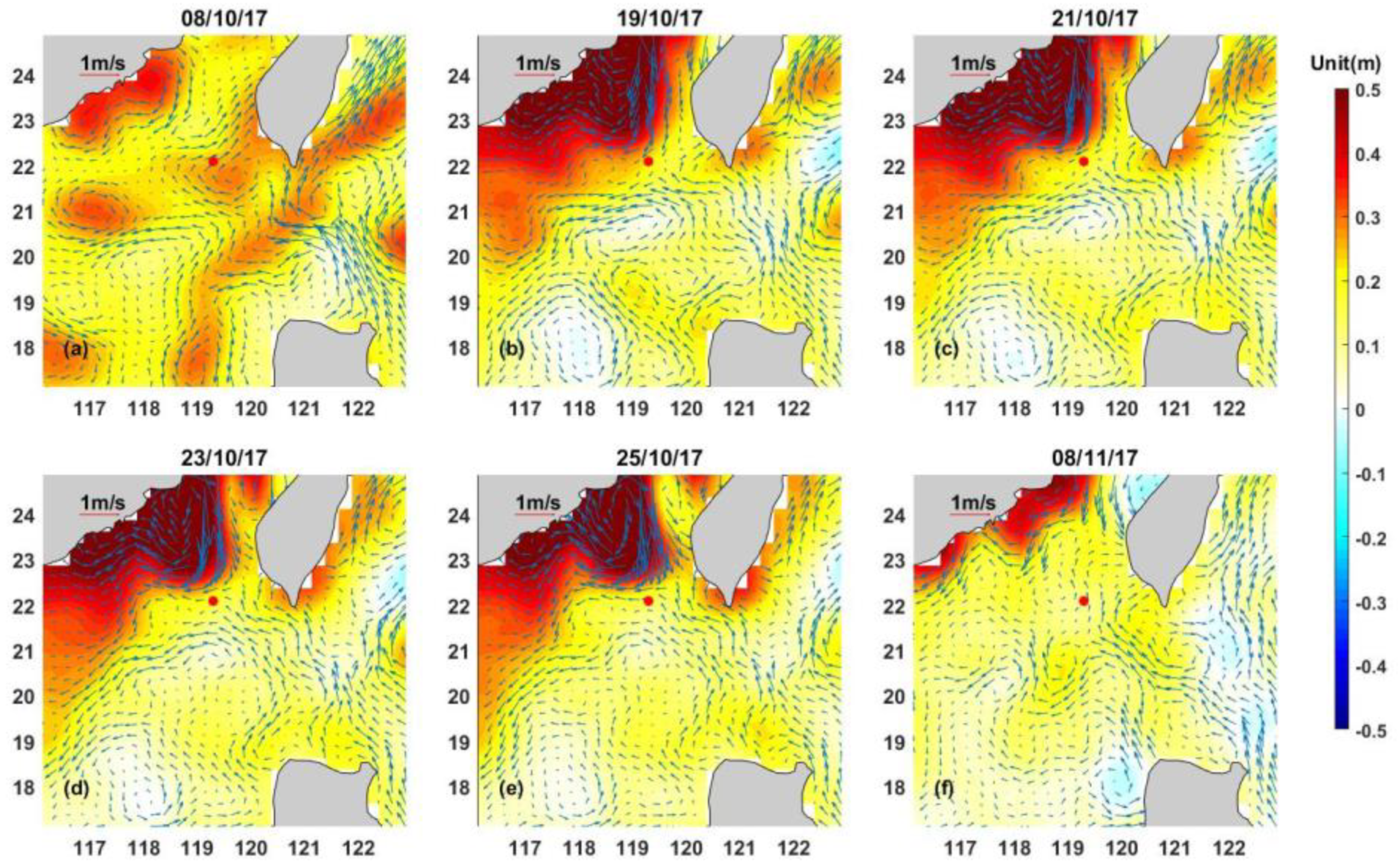
4.3. Subinertial Currents

In the previous sections, we described the characteristics of NIWs generated by typhoons. NIKE was seen at the observation depth least 28 days after the typhoon passed. PSI had no effect in the observation area. NIWs generated by SICs will be discussed in this section. There are two ways for SICs to generate NIWs. The first way is to destroy the geostrophic balance after crossing the potential vorticity isopleth. The fluid will generate NIWs to restore the geostrophic balance. This process is called Rossby adjustment [20]. The other way is the friction between the strong geostrophic current and the seabed topography. This process is called a Lee wave [37]. In this section, we determine whether ND and NE are affected by SIC by analyzing the characteristics.

Figure 8 shows the SIC characteristics of low-pass filtering with a timeframe of less than three days in the observation period. Figure 8a shows the depth–time distribution of kinetic energy. Figure 8b shows the depth average of subinertial kinetic energy (SIKE) and NIKE. During the entire observation period of Lander, two strong SIKEs occurred (Figure 8b). The two strongest SIKEs occurred on 26 September and 21 October, and they were unique throughout the observation period. Except for these two strong SIKEs, the third strong SIKE could not reach half of the energies during these two times. Coincidentally, both ND and NE occurred 18 days after these two events (Figure 8b). Since the attenuation of SIKE affected the potential vorticity contour, Rossby adjustment occurred [20], resulting in NIWs events. Therefore, these two strong SIKE events must be related to ND and NE. The position of the maximum value of SIKE was different in the two times, which means that the two NIWs events generations had different generation mechanisms. To analyze the impact of these two characteristics in detail, a feather diagram of the SIC during the two strong SIKE observations is shown in Figure 9, and the AVISO satellite data are combined to analyze whether the surface circulation affects the observation SIC of water depth.

To simplify the name of the two events, we named the strong SIKE phenomenon that occurred in September S9 and the phenomenon that occurred in October S10. By comparing the two graphs in Figure 9, many different SIC features between S9 and S10 can be found. Firstly, the strongest SIKE during S9 occurred in the deepest layer of the observed water depth interval, which was close to the seabed. The maximum SIKE was 30.78 J m⁻³, which occurred at a depth of 1085 m. The strongest SIKE during S10 occurred at the shallowest depth of the observation area. The maximum SIKE was 20.35 J m⁻³, which occurred at a depth of 655 m. Although the water depth average SIKE of S9 and S10 was not much different, the maximum value of the spatial distribution differed by more than 10 J m⁻³. Secondly, during S9, the direction of the velocity of the surface layer was basically opposite to the direction of the velocity of the observed water depth. During S10, the two were basically the same.

The S10 closest to the NE event was analyzed first. As shown in Figure 9, the flow velocity distribution during S10 and S9 was different. The surface velocity and the direction of the velocity of the water depth from 600 m to 1050 m were the same during S10. This shows that the surface flow field was barotropic, and the surface flow field can reflect the spatial transformation of the bottom flow. Therefore, the generation characteristics and mechanism of S10 could be analyzed by observing the changes in the sea surface current field. However, S9 cannot be analyzed this way. The sea level abnormally (SLA) during S10 is plotted in Figure 10. SLA and velocity anomalies were selected and plotted in Figure 10. Figure 10 shows that the strong SIKE of S10 originates from the coastal shelf wave (SCW) near the Chinese mainland. CSWs are subinertial waves generated by large-scale weather systems moving along or across the continental shelf [38,39,40,41,42]. This CSW exhibited a centimeter-level amplitude, a period close to one month and a wavelength of approximately one hundred kilometers, which was similar to previous CSW results [40,43]. This CSW was generated on October 8th (Figure 10a), expanded to its maximum range on October 21st (Figure 10c), and then decayed on November 8th (Figure 10f). The range of Lander can be affected from 19–25 October (Figure 10b–e), so SLA on 8, 19, 21, 23, 25 October and 8 November were selected in Figure 10. By combining the results of the Lander currents, the CSW was very strong at this time, and the flow field structure directly affected the seabed. The energy generated by the attenuation of this strong coastal shelf wave stimulated the Rossby adjustment in the nearby sea area. This process generates NIWs. In order to verify that our theory is correct, we estimated the signal in the middle layer of NE and the signal in the bottom layer, and found that the signal in the middle layer propagates horizontally, and the downward group velocity of the signal in the deep layer is 17 m d⁻¹. These two velocities, when multiplied by 18 days, correspond exactly to the attenuation of SIKE at 700 m and 900 m. That is to say, the SIKE attenuation at a water depth of 700 m produces the signal at the bottom of the NE, and the signal propagated horizontally in the middle layer is caused by the SIKE attenuation at 900 m. This could also explain why the horizontally propagating signal (middle layer signal) in the NE is earlier than the bottom layer signal.

4.4. Seabed Reflection

The NIWs event with NE below 900 m had its own unique characteristics. Through energy tracking, it was found that this part of the signal was caused by SIKE attenuation at a depth of about 700 m. In the meridional direction, NIWs events from 920 m to 1000 m appeared to propagate upwards. This feature was not found during the observation period, indicating that there was a special mechanism. The Lee wave generation method was excluded in areas below 900 m. Because it was the observation sea area to receive the Lee wave from outside, the time should be less than that from the shallow water location (18 days). However, no obvious features were found in the subinertial current within 18 days. Since the wave reflected when it touched the seabed, this part of the upward wave was the reflection of the NIWs energy. This phenomenon was not found in the zonal direction, indicating that under the influence of the terrain, the reflection of the NIWs event would appear to be anisotropic. However, although there was an upward energy transfer feature at NE below 900 m, there was no standing wave feature. This research task was required by two factors. First, the reflected upward energy was not equal to the original downward energy. Second, the observed NIWs had anisotropic characteristics, which made the incident signal different from the reflected signal and it could not form a standing wave. Previous studies, e.g., [44], modeled the reflected internal wave characteristics. If the observation position was at a certain distance from the reflection position, the strongest reflected energy did not occur on the seabed. Therefore, NE exhibited the characteristics of upward-propagating energy in certain water depth ranges (from 900 m to 985 m) and downward energy transmission in certain water depth ranges (from 1000 m to 1050 m).

4.5. Monsoons

The NE in the shallowest area and that of the NIWs event generated by typhoons have both common and different points. NE also had downward-propagation signals. However, the downward-propagation signal of NE was stronger than the NIWs event generated by the typhoon, and the phase difference between the zonal and meridional directions was not always 90 degrees. The NIWs event could be seen in the whole water depth of the observation area. This phenomenon was difficult to see in NIWs caused by typhoons. Notably, in the NIWs event shallower than 880 m, three distinct signals were found. The NE signal at a water depth of 820 to 880 m propagates horizontally and has a phase difference of 90 degrees. The NIWs events from 600 m to 720 m and signals from 740 m to 820 m were all transmitted downward. The signal in the upper layer (600–720 m) had a phase difference of 90 degrees, but the signal in the lower layer (740–820 m) was not. These three signals can be clearly found in Figure 4m. Through the previous results, we found that the NIWs generated by the typhoon had a phase difference of 90 degrees in the zonal and meridional directions and was characterized by downward energy transmission. At the same time, the phase difference of the ND produced by the SIKE attenuation was not 90 degrees, and the frequency signal was not stable. The signals in the upper layer were likely to originate from different formation mechanisms. Therefore, the characteristics of the winter monsoon were discussed in this study.

The winter monsoon, as a possible cause of NIWs, was discussed here. Figure 7c describes the change in wind kinetic energy during the observation period. From July to October, the wind kinetic energy could well reflect the changes in the wind field under the action of typhoons. Strong wind kinetic energy events would be produced after several typhoons. After October, although there was no longer a typhoon affecting the area where Lander was located, the winter monsoon from the northeast was strengthening. From the perspective of wind kinetic energy, it was obvious that the wind kinetic energy after October was much higher than that before October. This phenomenon was caused by the winter monsoon. Based on our previous research findings, it takes approximately 28 to 30 days to trace the NIWs events in the observed water depth to the strong wind kinetic energy of the typhoon. With this time interval as the standard, there was a strong winter monsoon 25 days before the occurrence of NE. This winter monsoon was also marked in Figure 7c. Since previous studies have shown that the summer monsoon produces an obvious NIWs event [18], the generation of NE was also inevitably related to the appearance of this winter monsoon. We estimate the downward group velocity of the shallowest layer of NE by NIKE, which is about 25m d⁻¹, which is slightly higher than the NIWs events generated by typhoons. Assuming that NIWs events were generated in the mixed layer (50 m water depth) 25 days ago, then energy propagation to 690 m at the NIKE maximum position requires a downward group velocity of approximately 25.6 m d⁻¹. This is consistent with the estimated NIKE group velocity.

During the formation of the shallowest layer of NE, there were two possible mechanisms of NIW. Firstly, through satellite and SIC research, there was a strong coastal shelf wave attenuation phenomenon on the ocean surface (Figure 10). This process generated Rossby adjustment. Secondly, the winter monsoon had a strong wind field phenomenon at this time (Figure 8c). The wind kinetic energy at this time exceeded the wind kinetic energy produced by the strongest typhoon. It is found that the time difference of 25 days can also just match the time of downward propagation by tracking NIKE. This winter monsoon also produced NIWs events. By comparing Figure 7b,c, it is found that the NIKE behind the NE does not have a significant correlation with the wind stress intensity of the winter monsoon, which indicates that the winter monsoon alone cannot generate NIWs events propagating this depth. It is worth noting that the NIWs signal at this depth has a stable signal, which is characteristic of the NIWs signal that propagates over long distances. Therefore, we conclude that the upper part of NE is generated due to the resonance between NIWs events generated by monsoons and NIWs generated by shelf waves. The reason why other monsoon-generated NIWs signals are not observed is that the resonance enhancement of other signals does not occur. Therefore, we concluded that the NIWs events in the upper layer were affected by two different generation mechanisms, forming three different NIWs events.

The attenuation of SIKE will produce horizontally propagating NIWs events, while the wind-generated NIWs event will propagate downward. Therefore, we know that NE’s horizontal propagation signal at a water depth of 820 to 880 m resulted from the energy obtained by SIKE attenuation. This phenomenon corresponds to the S10 attenuation at 900 m. The NIWs events from 600 m to 720 m and signals from 740 m to 820 m were all transmitted downward. The generation mechanism of the two parts of the signal could not only be judged by the downward-propagation feature. Since we know that the NIWs event is dispersive, the signal becomes increasingly consistent when signals are transmitted over a long distance. This phenomenon was particularly obvious in NA and NB generated by typhoons. Since the NIWs events from 600 m to 720 m had a phase difference of 90 degrees and correspond to the strengthening of the monsoon 25 days ago, this part of the signal was generated by the wind. Since the monsoon alone cannot generate NIWs events that travel more than 600 m, this energy was also affected by shelf wave attenuation to generate NIKE resonances. The signal from 740 m to 820 m does not have this characteristic, so it is caused by SIKE attenuation. In general, during the NE period, the NIWs event in the full water depth range can be divided into the NIWs event generated by the winter monsoon, in the water depth range of 600 to 720 m; the NIWs event generated by the shelf wave attenuation, in the range of all observation areas; and the NIWs event generated by the seabed reflection, in the range of 920 to 1000 m. The reflection signal was stronger in the zonal direction than in the meridional direction.

4.6. Lee Wave

The generation mechanism of Lee wave was not discussed. This is because, currently, the seafloor topography data we currently have cannot be made public. However, we observed that the generation of NDs was likely to be a Lee wave phenomenon.

We suspect that ND was a Lee waves mechanism for several reasons. Firstly, during S9, which is associated with the ND events, the SIC flows to the southwest, with a maximum at the bottom. If the ND comes from the Rossby adjustment caused by the direct SIKE attenuation, it was more likely that the NIWs event would transfer energy from the bottom to the top. This is different from the characteristics of ND, which is propagated horizontally. Secondly, the circulation during S9 also could not find obvious eddy features. Since eddies can affect the propagation direction of NIWs events, this indicates that the ND relay process did not encounter events that affect the internal wave characteristics and propagation direction. The observation found that the ND propagation is in the horizontal direction, which means that the generation position of ND is also in this water depth. This means that if the energy comes from the Rossby adjustment, then the SIKE would experience a significant change in energy decay in water depths of 700 to 800 m. This could be seen in Figure 9a that SIKE was attenuated, but the intensity was much less than the S10 phenomenon. Thus, it also shows that ND was not generated by Rossby adjustment. Thirdly, the shipboard Echo Sounder showed that there is a ridge with a depth of 800 m in the area northeast of Lander Station. Since these data are not sharable, they cannot be presented in this study. Considering that the strongest SIC at the bottom of the ocean was observed and upstream of the SIC encounters obstructions from submarine ridges, the generation of ND comes from the friction between the SIC and the ridge. Therefore, ND was likely NIWs events caused by the Lee wave mechanism.

5. Discussion

During the observation period, all strong NIWs events were analyzed. These events account for 47% of the total NIKE, and showed NIWs characteristics generated by typhoons, NIWs characteristics generated by monsoons, NIWs characteristics generated by Rossby adjustment, and NIWs characteristics generated by reflection. Since the currently obtained seabed topography data cannot be made public, it is impossible to discuss the NIWs phenomenon formed by the Lee wave, but we have made a reasonable speculation about the formation of the ND. In this study, by tracing the source of the NIWs propagation process, it was found that this event occurred at the seafloor ridge. This process deserves more analysis. The study found that there is a time interval of 18 days between the ND and the strong sub-inertial flow event, coinciding with the arrival time of the NIWs, as suggested in previous studies. However, the source of the NIKE of ND cannot be identified, as the propagation direction is not capable of capturing by a single station measurement of current profile. However, the temperature-salt structure given by WOA can obtain the phase velocity of the ideal wave, so that the NIWs can be simulated. This process is a very interesting physical phenomenon. Future research can try to analyze the ND phenomenon separately through this idea.

The energy reflectivity of the seafloor is still worth modeling, and only a significant upward signal at a distance between 940 m and 985 m was found in NE. However, NA, NB, NC, and NE found strong shear at depths of 900 m to 1000 m. ND occurs at water depths of 1000 to 1100 m. The signal was very likely to originate from the reflection of the seabed. However, from the NIKE study, only NE found the reflected signal and nothing else. At the same time, the reflected signal also shows obvious anisotropy, which is closely related to topography. These processes need to be clarified in future work.

6. Summary

Temporal and spatial patterns of NIKE were investigated in the Lander ADCP in the northeastern part of the South China Sea from July to November 2017. Lander was located at a depth of 1135 m under the sea. The ADCP sent signals upwards and could obtain flow field data from a depth of 600 m to 1100 m. The purpose was to (1) document the spatiotemporal distribution of near-inertial energy. (2) Determine the reason for the generation of the NIWs field in the existing data. (3) Determine the difference in NIWs events under different generation mechanisms. To calculate the NIWs frequency and vertical wavenumber more accurately, Sun’s method [27] is used here. The data support the following conclusions.

A total of five significant NIWs events were discovered during the observation period. These events were named NA, NB, NC, ND, and NE. Analyzing the temporal and spatial characteristics of five events, it was found that NA and NB have downward energy signals, and the signal characteristics are relatively stable. The main signals of NA and NB had a phase difference of 90 degrees in the zonal and meridional directions. In the NC main signal, the zonal and meridional directions no longer had the characteristics of vertical stability, and the energy transmission characteristics were no longer obvious. The vertical wavenumber of the ND main signal was close to zero, and the phase difference between the zonal and meridional directions was greater than 90 degrees. The frequency peak increases with water depth. Even in the depth range of 600 m to 1100 m, the mixed contribution of NIWs event was stronger than that of semidiurnal tides and diurnal tides. The shear in the zonal direction was slightly higher than that in the meridional direction. Among the five NIWs, the strongest shear occurred in NE because NE was stimulated by multiple factors. It is found the downstream signal at all water depths during NE, but the 90-degree phase difference did not continue to the full water depth. Shearing was generally strongest at water depths of 900 m to 1000 m close to the seabed, which was probably caused by terrain reflections. These five NIWs events had different characteristics, which means that different generation mechanisms and influencing factors existed during these five events.

The reasons for the generation of these five NIWs events were analyzed in this study. Typhoons are the primary consideration. Typhoons will inevitably generate NIWs, but whether the generated NIWs can be transmitted to deep water needs to be analyzed. Due to the depth of the observed area, there was a gap between the observed NIWs event time and the typhoon passing time. After analysis, two typical NIWs events, NA and NB, were caused by typhoons Roke and Haitang. The intervals between typhoons and NIWs were 28 days and 30 days, respectively. The estimated vertical group velocities of these two events at the observed positions and interval time just coincided with the vertical propagation velocities estimated by the phase vertical slope. The NIWs generated by the typhoon spread over a long time and distance, and its signal was uniform. The phase difference between the zonal and meridional directions stabilized at 90 degrees. At the same time, it had a negative vertical wavenumber in which energy was transmitted downward. Although NC coincides well with the typhoon period, NC did not have the above characteristics, so it is known that NC was not directly caused by the typhoon. Other possible formation causes of NC were also explored. It was found that neither PSI, monsoon, nor background flow weakening could be responsible for the generation of NC. Thus, NC can only occur by spontaneous generation.

The characteristics of NE were the strongest among the five events. The attenuation characteristic of SIKE appeared 18 days before NE was generated. This feature could be verified as a shelf wave event by the sea surface height. Because the NE excitation source was above the observation, energy was transmitted downward. At the same time, the strength of the wind field was also found 25 days before NE generation. By tracking NIKE, it was found that the 25 days and the time of NIWs downward generated by the monsoon can correspond, so monsoon also contributed to the generation of NE. According to NE’s characteristic analysis, the signal between 600 m and 720 m was generated by monsoon. It can be transmitted deeper than other monsoon-generated NIWs events due to the Rossby adjustment resonance. It had the characteristics of energy downward propagation and had a phase difference of 90 degrees. The signal below 740 m was generated by SIKE. Some parts of the energy can be tracked to find their corresponding Rossby adjustment positions. Its energy sometimes transmitted horizontally and sometimes transmitted downward, the phase difference was not 90 degrees. The signal between 940 m and 1050 m contains the signal reflected from the seafloor. The reflected signal was only observed in the meridional direction, which is due to the complex seafloor topography.

ND had the characteristics of horizontal transmission. Through analysis of the generation mechanism, ND was generated by SIKE. A strong SIKE phenomenon occurred 18 days before ND was generated. In this strong SIKE phenomenon, the strongest energy did not appear at the shallowest part of the observations, but around 800 m of water. Tracing the source of the energy revealed no obvious Rossby adjustment areas. Combined with the seafloor topography data, we found that there is a ridge approximately 800 m upstream of the current field. Since data on the topography of the seafloor cannot be shared, further research is difficult. Thus, in this study, it is speculated that ND was probably caused by the interaction between SIC and ridges. In addition to the horizontal propagation characteristic of the generated ND, the phase difference between the zonal and meridional directions was not 90 degrees, which differed from the NIWs event directly generated by a typhoon. This is because the horizontally propagating NIWs events have only two-dimensional dispersion characteristics, which are weaker than the wind-generated NIWs characteristics of three-dimensional dispersion. This results in signals of multiple frequencies still appearing simultaneously, rather than being spread out like three-dimensional dispersion. Therefore, the observed frequency was not constant along the water depth, but increases, and the phase difference between the zonal and meridional directions is not 90 degrees, which shows that the ND includes different horizontal propagation signal components.

References

1. Fu, L.L. Observations and models of inertial waves in the deep ocean. Rev. Geophys. 1981, 19, 141–170. [Google Scholar] [CrossRef] [Green Version]
2. Alford, M.H.; MacKinnon, J.A.; Simmons, H.L.; Nash, J.D. Near-inertial internal gravity waves in the ocean. Annu. Rev. Mar. Sci. 2016, 8, 95–123. [Google Scholar] [CrossRef] [Green Version]
3. Le Boyer, A.; Alford, M.H.; Pinkel, R.; Hennon, T.D.; Yang, Y.J.; Ko, D.; Nash, J. Frequency shift of near-inertial waves in the South China Sea. J. Phys. Oceanogr. 2020, 50, 1121–1135. [Google Scholar] [CrossRef] [Green Version]
4. MacKinnon, J.A.; Gregg, M.C. Near-inertial waves on the New England shelf: The role of evolving stratification, turbulent dissipation, and bottom drag. J. Phys. Oceanogr. 2005, 35, 2408–2424. [Google Scholar] [CrossRef] [Green Version]
5. Van der Lee, E.M.; Umlauf, L. Internal wave mixing in the Baltic Sea: Near-inertial waves in the absence of tides. J. Geophys. Res. Ocean. 2011, 116. [Google Scholar] [CrossRef]
6. Lucas, A.J.; Pitcher, G.C.; Probyn, T.A.; Kudela, R.M. The influence of diurnal winds on phytoplankton dynamics in a coastal upwelling system off southwestern Africa. Deep. Sea Res. Part II Top. Stud. Oceanogr. 2014, 101, 50–62. [Google Scholar] [CrossRef]
7. Guan, S.; Zhao, W.; Huthnance, J.; Tian, J.; Wang, J. Observed upper ocean response to typhoon Megi (2010) in the Northern South China Sea. J. Geophys. Res. Ocean. 2014, 119, 3134–3157. [Google Scholar] [CrossRef] [Green Version]
8. Hou, H.; Yu, F.; Nan, F.; Yang, B.; Guan, S.; Zhang, Y. Observation of near-inertial oscillations induced by energy transformation during typhoons. Energies 2019, 12, 99. [Google Scholar] [CrossRef] [Green Version]
9. Wang, G.; Li, D.; Wei, Z.; Li, S.; Wang, Y.; Xu, T. Observed Near Inertial Waves in the Wake of Typhoon Linfa (2015) in the Northern South China Sea. J. Ocean. Univ. China 2019, 18, 1013–1021. [Google Scholar] [CrossRef]
10. MacKinnon, J.A.; Winters, K.B. Subtropical catastrophe: Significant loss of low-mode tidal energy at 28.9°. Geophys. Res. Lett. 2005, 32. [Google Scholar] [CrossRef] [Green Version]
11. Xie, X.H.; Shang, X.D.; van Haren, H.; Chen, G.Y.; Zhang, Y.Z. Observations of parametric subharmonic instability-induced near-inertial waves equatorward of the critical diurnal latitude. Geophys. Res. Lett. 2011, 38. [Google Scholar] [CrossRef] [Green Version]
12. Nikurashin, M.; Ferrari, R. Radiation and dissipation of internal waves generated by geostrophic motions impinging on small-scale topography: Theory. J. Phys. Oceanogr. 2010, 40, 1055–1074. [Google Scholar] [CrossRef]
13. Hu, Q.; Huang, X.; Zhang, Z.; Zhang, X.; Tian, J. Cascade of internal wave energy catalyzed by eddy-Topography interactions in the deep South China Sea. Geophys. Res. Lett. 2020, 47, e2019GL086510. [Google Scholar] [CrossRef]
14. Ford, R. Gravity wave radiation from vortex trains in rotating shallow water. J. Fluid Mech. 1994, 281, 81–118. [Google Scholar] [CrossRef]
15. Jaimes, B.; Shay, L.K. Near-inertial wave wake of Hurricanes Katrina and Rita over mesoscale oceanic eddies. J. Phys. Oceanogr. 2010, 40, 1320–1337. [Google Scholar] [CrossRef]
16. Chen, G.; Xue, H.; Wang, D.; Xie, Q. Observed near-inertial kinetic energy in the northwestern South China Sea. J. Geophys. Res. Ocean. 2013, 118, 4965–4977. [Google Scholar] [CrossRef] [Green Version]
17. Xu, J.; Huang, Y.; Chen, Z.; Liu, J.; Liu, T.; Li, J.; Ning, D. Horizontal variations of typhoon-forced near-inertial oscillations in the south China sea simulated by a numerical model. Cont. Shelf Res. 2019, 180, 24–34. [Google Scholar] [CrossRef]
18. Shu, Y.; Pan, J.; Wang, D.; Chen, G.; Sun, L.; Yao, J. Generation of near-inertial oscillations by summer monsoon onset over the South China Sea in 1998 and 1999. Deep. Sea Res. Part I Oceanogr. Res. Pap. 2016, 118, 10–19. [Google Scholar] [CrossRef]
19. Ma, Y.; Zhang, S.; Qi, Y.; Jing, Z. Upper ocean near-inertial response to the passage of two sequential typhoons in the northwestern South China Sea. Sci. China Earth Sci. 2019, 62, 863–871. [Google Scholar] [CrossRef]
20. Rossby, C.G. On the mutual adjustment of pressure and velocity distributions in certain simple current systems, II. J. mar. Res. 1938, 1, 239–263. [Google Scholar] [CrossRef]
21. Hoskins, B.J.; Bretherton, F.P. Atmospheric frontogenesis models: Mathematical formulation and solution. J. Atmos. Sci. 1972, 29, 11–37. [Google Scholar] [CrossRef] [Green Version]
22. Snyder, C.; Skamarock, W.C.; Rotunno, R. Frontal dynamics near and following frontal collapse. J. Atmos. Sci. 1993, 50, 3194–3212. [Google Scholar] [CrossRef]
23. Plougonven, R.; Snyder, C. Inertia–gravity waves spontaneously generated by jets and fronts. Part I: Different baroclinic life cycles. J. Atmos. Sci. 2007, 64, 2502–2520. [Google Scholar] [CrossRef] [Green Version]
24. Danioux, N. Bilan des Campagnes Océanographiques Françaises 2012, French Oceanographic Cruises Report. IFREMER. 2013. Available online: https://archimer.ifremer.fr/doc/00149/26002/ (accessed on 1 March 2022).
25. Shakespeare, C.J.; Taylor, J.R. The spontaneous generation of inertia–gravity waves during frontogenesis forced by large strain: Theory. J. Fluid Mech. 2014, 757, 817–853. [Google Scholar] [CrossRef]
26. Nagai, T.; Tandon, A.; Kunze, E.; Mahadevan, A. Spontaneous generation of near-inertial waves by the Kuroshio Front. J. Phys. Oceanogr. 2015, 45, 2381–2406. [Google Scholar] [CrossRef]
27. Xu, Z.; Yin, B.; Hou, Y.; Xu, Y. Variability of internal tides and near-inertial waves on the continental slope of the northwestern South China Sea. J. Geophys. Res. Ocean. 2013, 118, 197–211. [Google Scholar] [CrossRef]
28. Sun, Z.; Hu, J.; Zheng, Q.; Gan, J. Comparison of typhoon-induced near-inertial oscillations in shear flow in the northern South China Sea. Acta Oceanol. Sin. 2015, 34, 38–45. [Google Scholar] [CrossRef]
29. Cao, A.; Guo, Z.; Song, J.; Lv, X.; He, H.; Fan, W. Near-inertial waves and their underlying mechanisms based on the South China Sea internal wave experiment (2010–2011). J. Geophys. Res. Ocean. 2018, 123, 5026–5040. [Google Scholar] [CrossRef]
30. Sun, L.; Zheng, Q.; Wang, D.; Hu, J.; Tai, C.K.; Sun, Z. A case study of near-inertial oscillation in the South China Sea using mooring observations and satellite altimeter data. J. Oceanogr. 2011, 67, 677–687. [Google Scholar] [CrossRef]
31. Yang, B.; Hou, Y.; Hu, P.; Liu, Z.; Liu, Y. Shallow ocean response to tropical cyclones observed on the continental shelf of the northwestern South China Sea. J. Geophys. Res. Ocean. 2015, 120, 3817–3836. [Google Scholar] [CrossRef]
32. Kim, Y.C.; Powers, E.J. Digital bispectral analysis and its applications to nonlinear wave interactions. IEEE Trans. Plasma Sci. 1979, 7, 120–131. [Google Scholar] [CrossRef]
33. Alford, M.H.; Whitmont, M. Seasonal and spatial variability of near-inertial kinetic energy from historical moored velocity records. J. Phys. Oceanogr. 2007, 37, 2022–2037. [Google Scholar] [CrossRef]
34. Sun, Z.; Hu, J.; Zheng, Q.; Li, C. Strong near-inertial oscillations in geostrophic shear in the northern South China Sea. J. Oceanogr. 2011, 67, 377–384. [Google Scholar] [CrossRef]
35. McComas, C.H.; Briscoe, M.G. Bispectra of internal waves. J. Fluid Mech. 1980, 97, 205–213. [Google Scholar] [CrossRef]
36. Carter, G.S.; Gregg, M.C. Persistent near-diurnal internal waves observed above a site of M2 barotropic-to-baroclinic conversion. J. Phys. Oceanogr. 2006, 36, 1136–1147. [Google Scholar] [CrossRef]
37. St Laurent, L.; Naveira Garabato, A.C.; Ledwell, J.R.; Thurnherr, A.M.; Toole, J.M.; Watson, A.J. Turbulence and diapycnal mixing in Drake Passage. J. Phys. Oceanogr. 2012, 42, 2143–2152. [Google Scholar] [CrossRef] [Green Version]
38. Robinson, A.R. Continental shelf waves and the response of sea level to weather systems. J. Geophys. Res. 1964, 69, 367–368. [Google Scholar] [CrossRef]
39. Mysak, L.A.; Hamon, B.V. Low-frequency sea level behavior and continental shelf waves off North Carolina. J. Geophys. Res. 1969, 74, 1397–1405. [Google Scholar] [CrossRef]
40. Adams, J.K.; Buchwald, V.T. The generation of continental shelf waves. J. Fluid Mech. 1969, 35, 815–826. [Google Scholar] [CrossRef]
41. LeBlond, P.H.; Mysak, L.A. Waves in the Ocean; Elsevier: Amsterdam, The Netherlands, 1981. [Google Scholar]
42. Thiebaut, S.; Vennell, R. Observation of a fast continental shelf wave generated by a storm impacting Newfoundland using wavelet and cross-wavelet analyses. J. Phys. Oceanogr. 2010, 40, 417–428. [Google Scholar] [CrossRef]
43. Schumann, E.H.; Brink, K.H. Coastal-trapped waves off the coast of South Africa: Generation, propagation and current structures. J. Phys. Oceanogr. 1990, 20, 1206–1218. [Google Scholar] [CrossRef] [Green Version]
44. Wang, G.; Zheng, Q.; Lin, M.; Dai, D.; Qiao, F. Three dimensional simulation of internal wave attractors in the Luzon Strait. Acta Oceanol. Sin. 2015, 34, 14–21. [Google Scholar] [CrossRef]
Figure 1. (a) Deployment of the Lander research in 2017. Lander was moored near the Luzon Strait. During the 2017 Lander component, the measurement location was approximately 177 km northwest of the strait in the sea area of the Kuroshio invasion. Lander was placed at approximately 1135 m water depth in 2017. All typhoon paths passed during the observation period are also plotted in different colors. The name of each typhoon is marked next to the typhoon track. (b) Schematic of acoustic Doppler current profiler (ADCP) instrumentation using during Lander data acquisition. The ADCP recorded horizontal velocities with an approximately 8 m vertical resolution.
Jmse 10 00594 g001
Figure 2. Near-inertial current velocity profiles. In (a,b) are shown the U and V components, respectively. The bandpass range used is from 0.8 f0 to 1.2 f0. The gray vertical lines in the figure mark the extent of each NIWs event.
Jmse 10 00594 g002
Figure 3. (a) Depth–time map of near-inertial kinetic energy (NIKE) per unit of volume, NIKE = 0.5ρ(uf2 + vf2) (J/m3), and (b) depth-averaged components. The shaded area represents a significant near-inertial signal. The names of these five phenomena are marked in the shaded area.
Jmse 10 00594 g003
Figure 4. (a,d,g,j,m) The depth distribution of the frequency for NA, NB, NC, ND, and NE. (b,e,h,k,n) The depth distribution of the phase for NA, NB, NC, ND, and NE. (c,f,i,l,o) Depth–time map of the NIKE for NA, NB, NC, ND, and NE. The blue points indicate the zonal velocity (U) result, and the red points indicate the meridional velocity (V) result. Color bar units are J m−3. To better discover the depth change in the phase, we drew a mark for the part from −180° to 0° a second time and placed it between 180° and 360° using asterisks and circles.
Jmse 10 00594 g004
Figure 5. (a) The shear of NIW, diurnal and semidiurnal tides during the observation period. Red represents NIWs shear. Magenta represents diurnal tide shear. Blue represents the semidiurnal tide. The solid line represents the zonal direction. The dashed line represents the meridional direction. (b) Vertical shear in the zonal direction averaged every 100 m. Different colors represent different water depths, marked in the figure. (c) The same as (b), but for the meridional direction.
Jmse 10 00594 g005
Figure 6. All typhoons characteristic energy with the closest distance of less than 20 km after July 2017. The data are selected from the Japan Meteorological Agency. There were five typhoons that met this condition: Roke, Haitang, Hato, Mawar, and Guchol. Figure (a) shows the time series of distance between the Lander and five typhoons. (b) The moving speeds of the centers of the five typhoons. The red dots in (a) mark the time corresponding to the nearest locations of the typhoon and Lander. At the same time, the corresponding times in (b) are marked in this figure. Figure (c) shows the characteristics of wind kinetic energy during this period. The data are derived from CCMP wind field data. (d) The depth average of NIKE, and the time interval is selected from 25 July to 1 October. The closest times to Lander of four typhoons, Roke, Haitang, Hato, and Mawar, which produced NIWs, are also marked with orange circles. The gray line marks the time when NIKE is strongest. The red dashed lines represent the time between the typhoons and the maximum value of NIKE. The specific times are also marked in (d).
Jmse 10 00594 g006
Figure 7. Bicoherence value in the frequency bin corresponding to PSI (FM2 = f + FM2 − f) plotted as a function of depth. The vertical dashed lines give the 80%, 90%, and 95% significance levels. Figure (a) corresponds to the NC period, Figure (b) corresponds to the ND period, and Figure (c) corresponds to the NE period.
Jmse 10 00594 g007
Figure 8. (a) Depth–time map of subinertial kinetic energy. Color bar units are J m−3. (b) Depth averages of subinertial kinetic energy and NIKE. The light blue dashed line represents the time of maximum ND and NE NIKE. The orange dotted line represents the time of maximum subinertial kinetic energy. The time difference between the maximum NIKE and maximum subinertial kinetic energy is also marked on the graph. (c) Surface wind kinetic energy. The light blue broken line represents the time of maximum NE NIKE. The orange dotted line represents the time of maximum wind kinetic energy. The time difference between the maximum NIKE and wind kinetic energy is also marked on the graph.
Jmse 10 00594 g008
Figure 9. Spatiotemporal distribution of subinertial kinetic energy from 20 September to 3 October (a) and from 12 October to 2 November (b). Feather chart of subinertial velocity from 20 September to 3 October (c) and from 12 October to 2 November (d). Lander data are used for the 600–1100 m data. The surface data are illustrated by AVISO satellite surface flow field data at the Lander location.
Jmse 10 00594 g009
Figure 10. Sea level anomaly (SLA) on 8th October (a), 19th (b), 21st (c), 23rd (d), 25th (e) and 8th November (f). The unit of the color bar is meters. The standard flow velocity of one meter per second is shown on the upper right of each graph. The red dot marks the location of Lander.
Jmse 10 00594 g010