
Fluid-Structure Interaction of a Foiling Craft

 , ,
, ,
Abstract
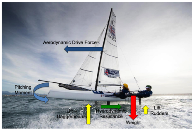
:1. Introduction
- Adjusting the weight of the crews that constantly move along the hull;
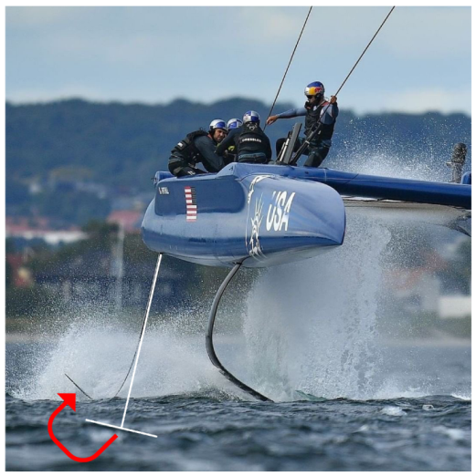
- Actively changing the rake angle of the daggerboards with a range of to . This can be done with a series of pulley systems whilst sailing. The daggerboards can be independently moved, giving the possibility of having the windward and leeward daggerboard on different and even opposing rake angles;
- Adjusting the rake of the T-rudders whilst stationary on land or in between races. The rake range in the rudders varies approximately between to .
2. Background on Fluid-Structure Interaction
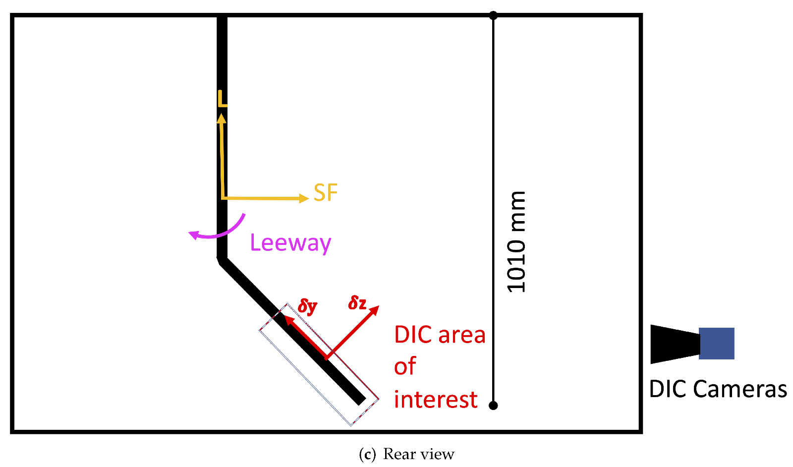
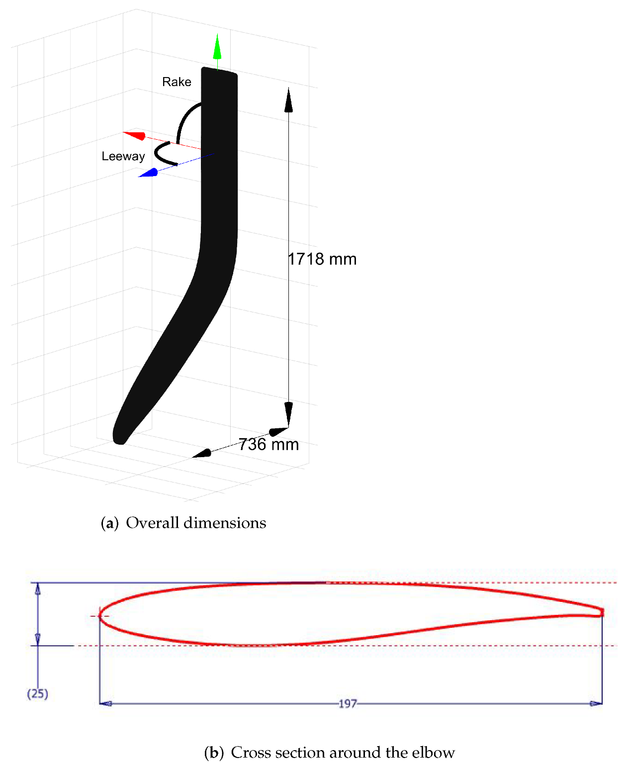
3. Geometries and Reference Systems
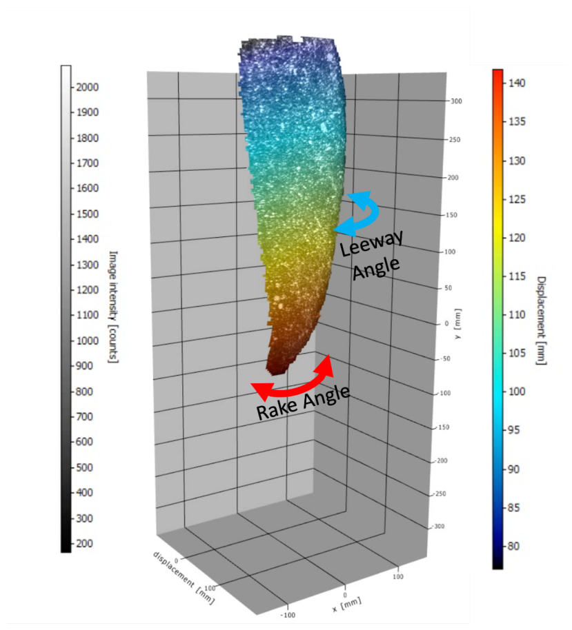
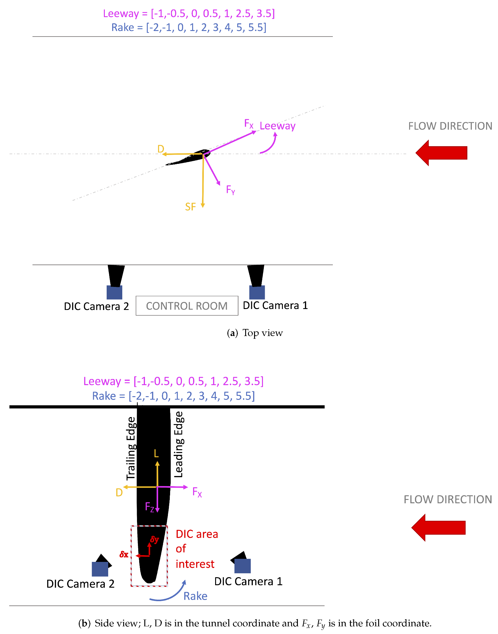
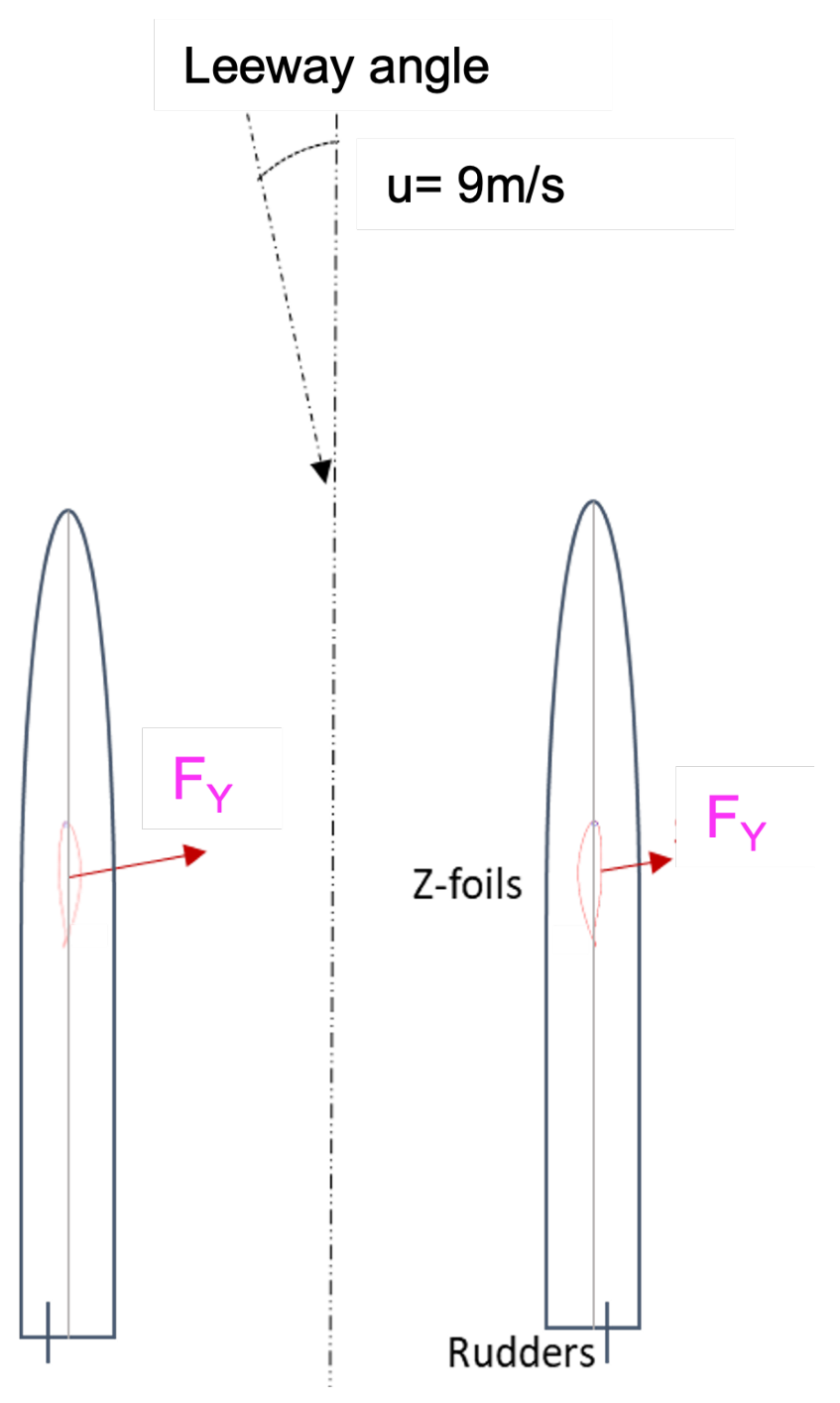
- Leeway angle: T = ;
- Rake angle: R = ;
- Speed: U = 5 m/s, 7 m/s, 9 m/s.
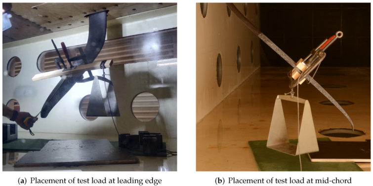
4. Experimental Setup
5. Computational Methods
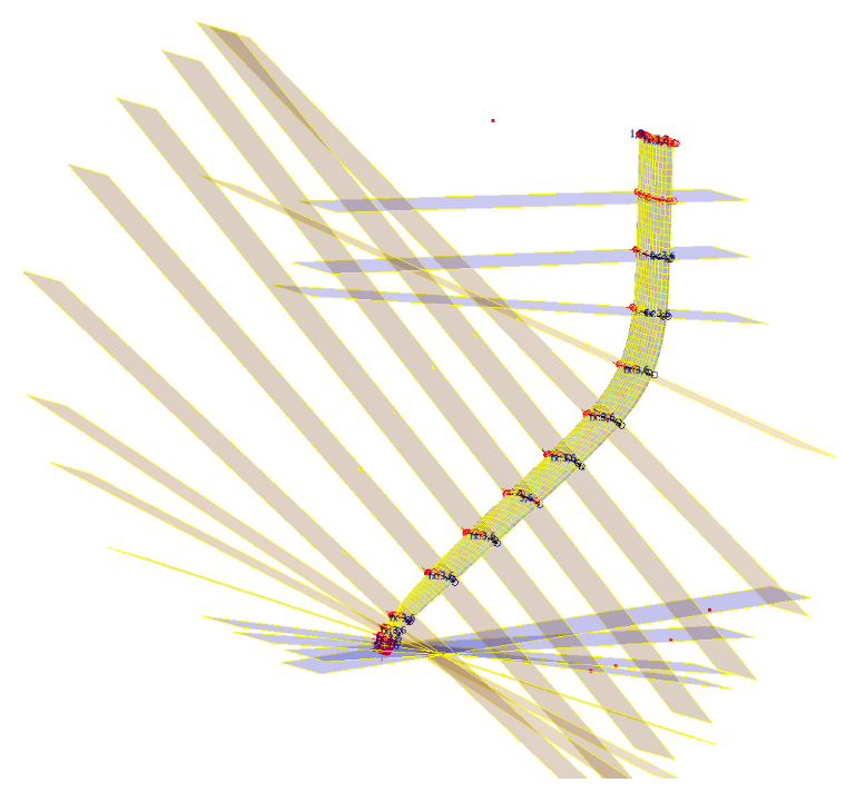
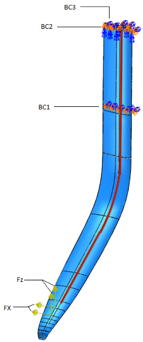
5.1. Finite Element Analysis
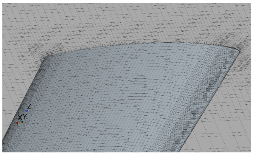
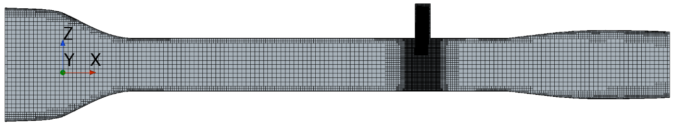
5.2. Computational Fluid Dynamics
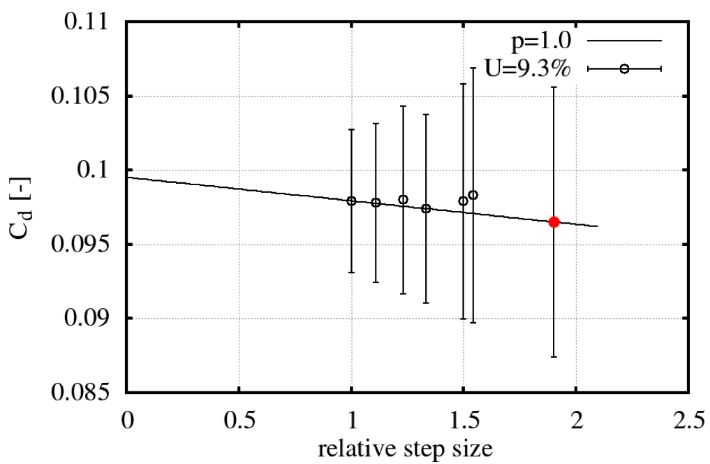
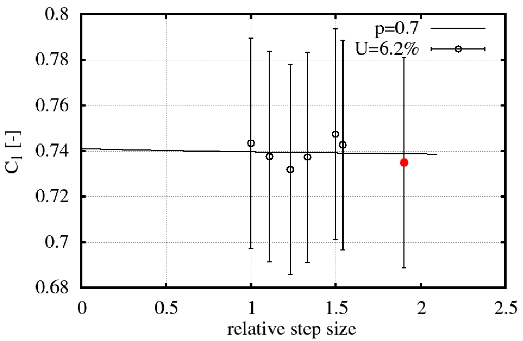
Verification
6. Discussion of the Results
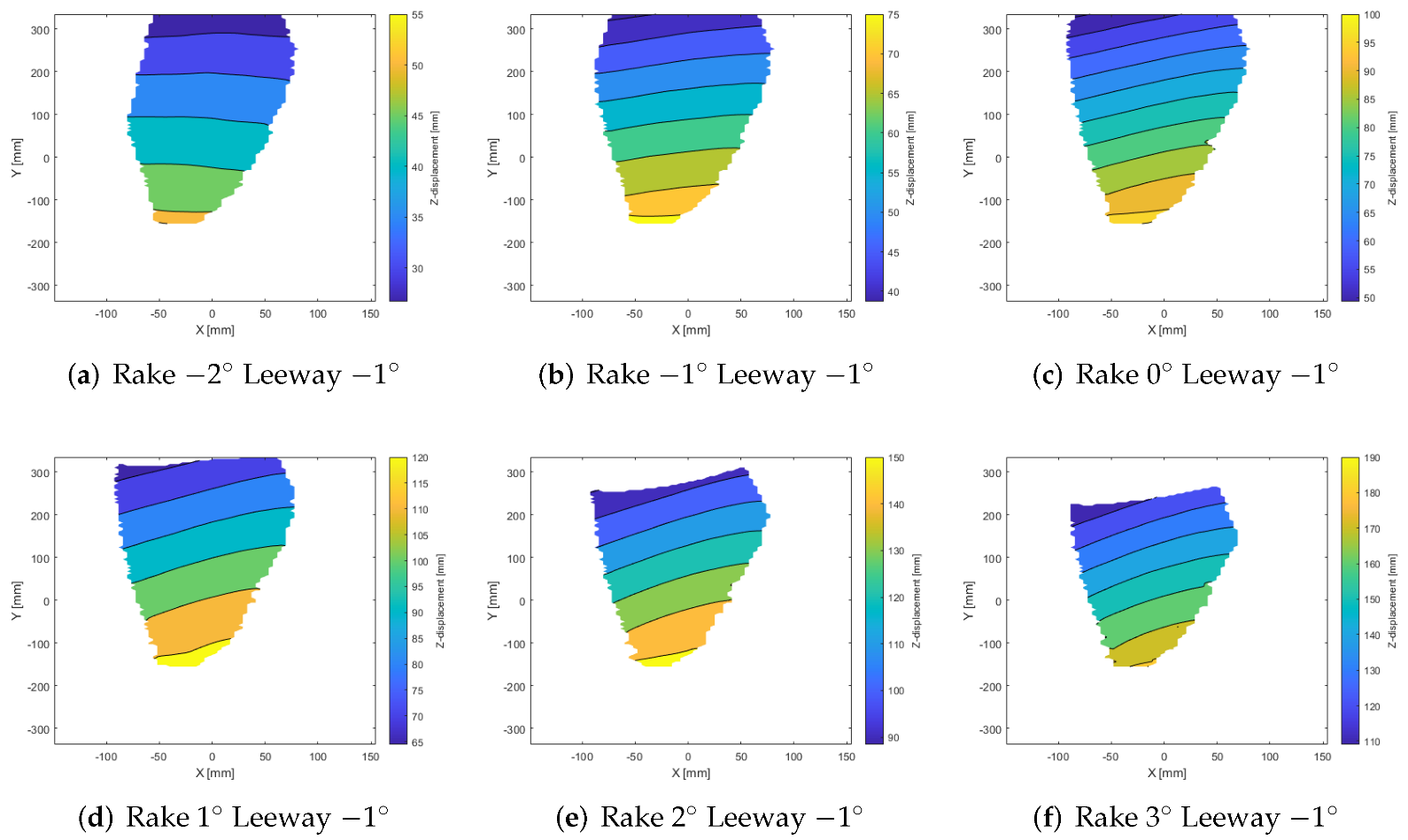
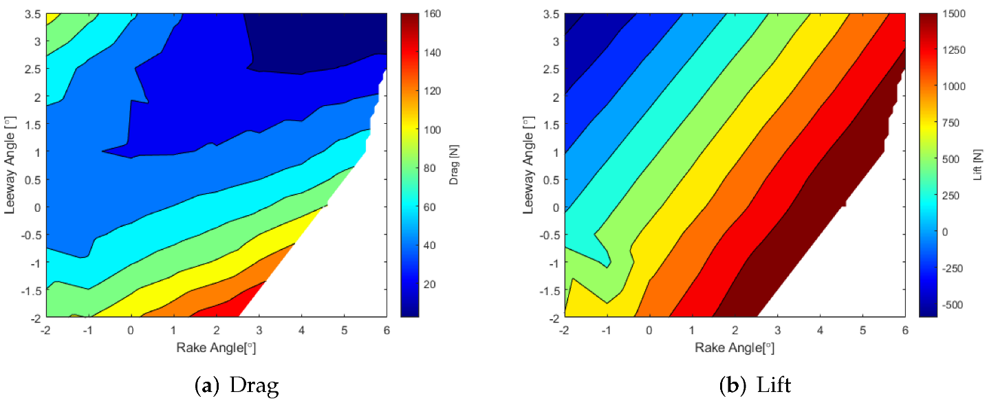
6.1. Experimental Results
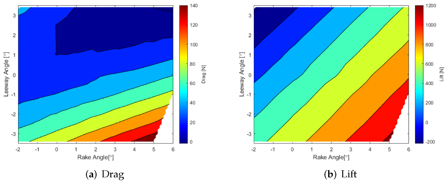
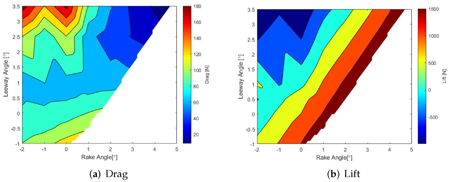
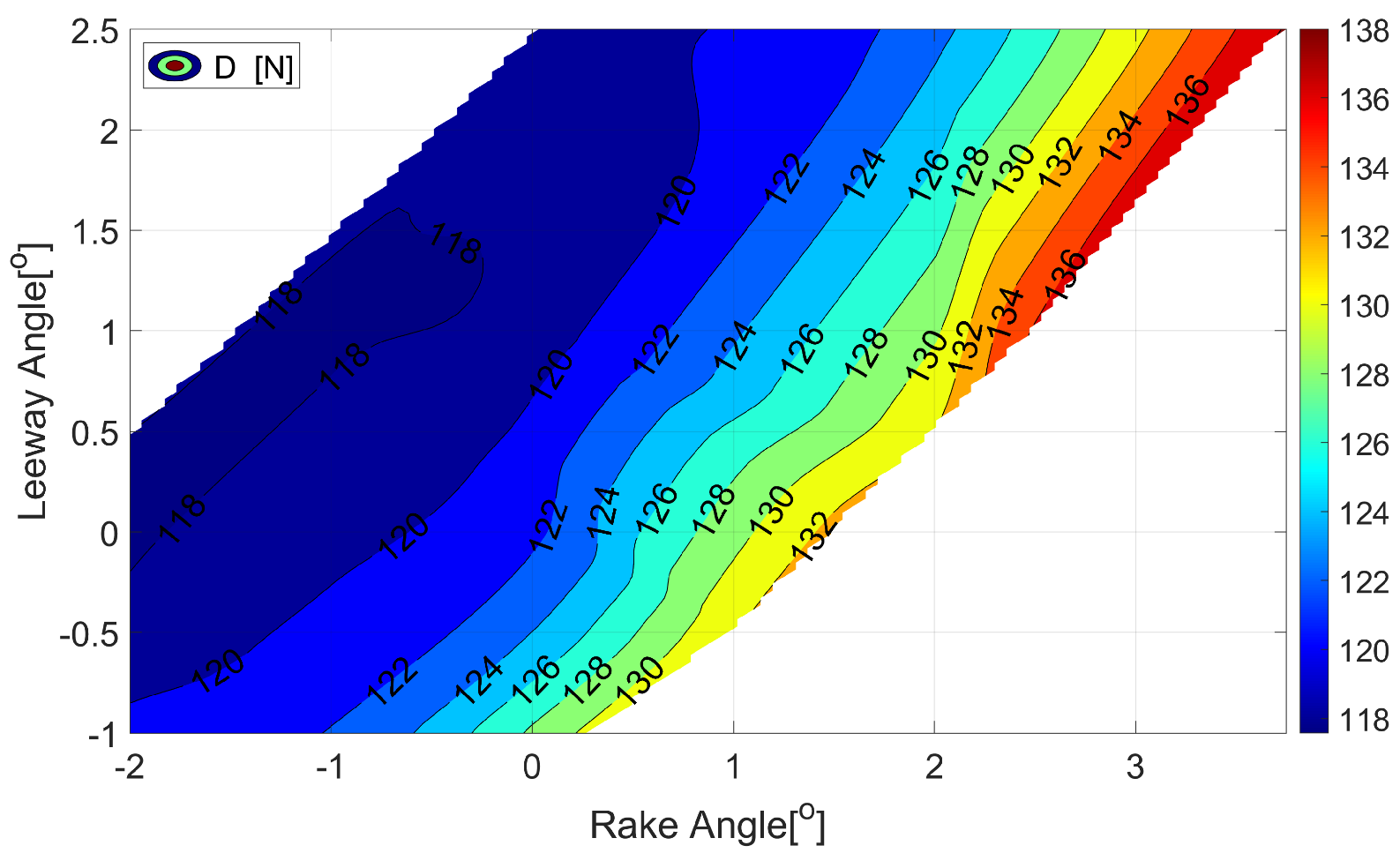
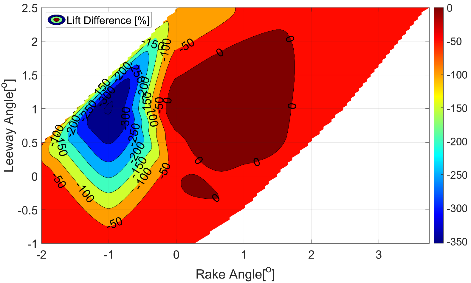
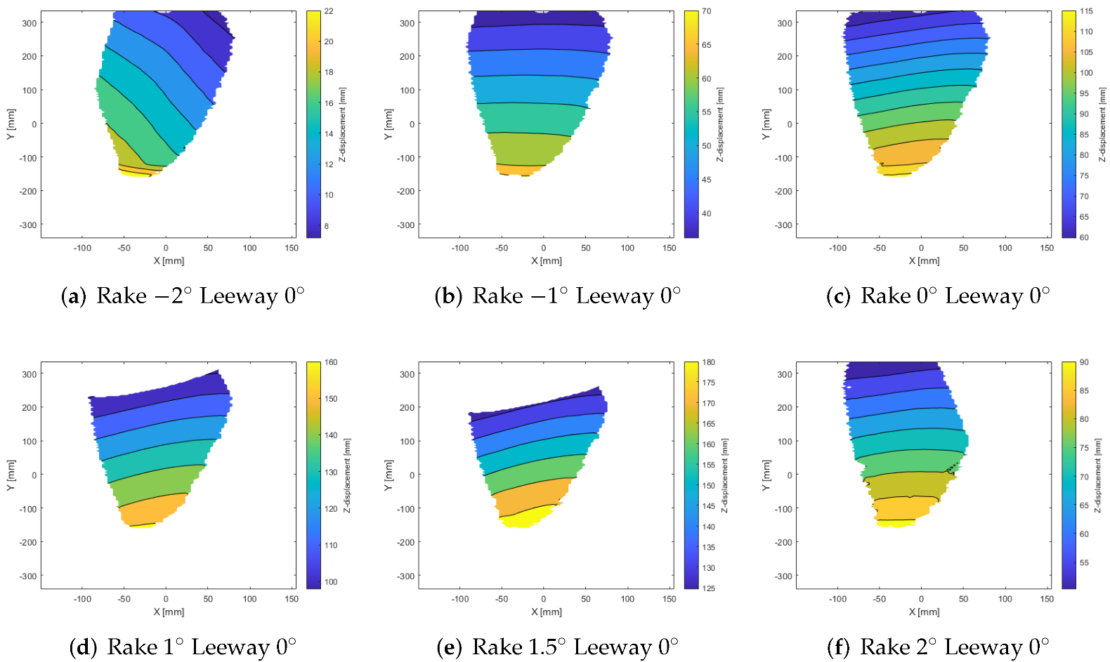
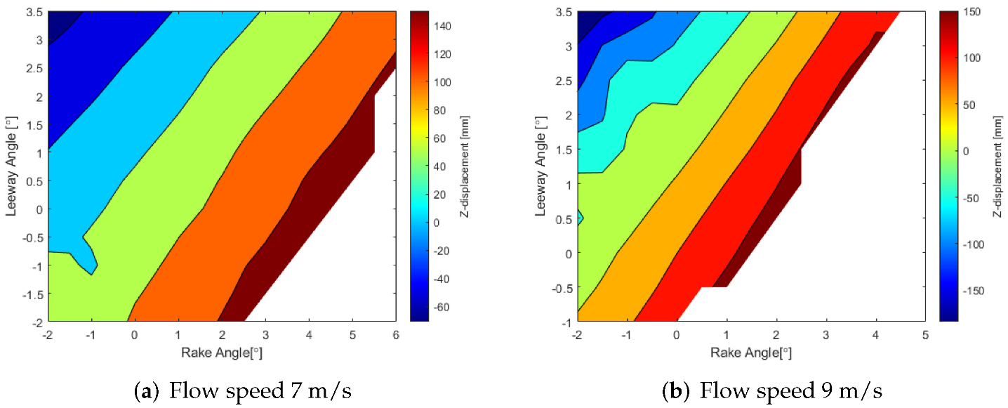
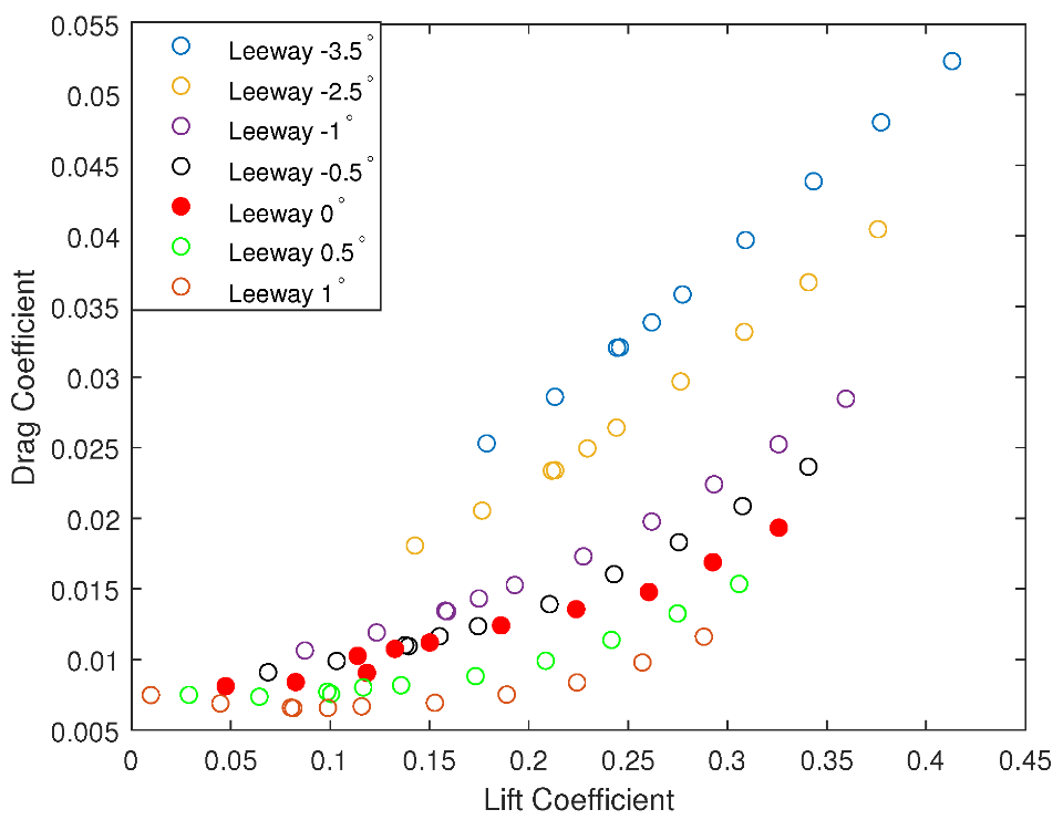
6.2. Numerical Results
7. Conclusions
Author Contributions
Funding
Institutional Review Board Statement
Informed Consent Statement
Acknowledgments
Conflicts of Interest
References
- NACRA Sailing. NACRA 17 Specifications. Available online: https://nacra17.org/nacra17/ (accessed on 7 June 2021).
- Guida, P.; Marimon Giovannetti, L.; Boyd, S.W. Three-dimensional variations of the NACRA 17 main foil for benchmarking shape optimizations. In Proceedings of the 5th International Conference on Innovation in High Performance Sailing Yachts and Sail-Assisted Ship Propulsion, INNOVSAIL, Gothenburg, Sweden, 15–17 June 2020. [Google Scholar]
- Marimon Giovannetti, L.; Stenius, I. Review of underwater Fluid-Structure Interaction measuring techniques. In Proceedings of the 7th High Performance Yacht Design Conference, Auckland, New Zealand, 11–12 March 2021. [Google Scholar]
- Bazilevs, Y.; Takizawa, K.; Tezduyar, T.E. Computational Fluid-Structure Interaction: Methods and Applications; Elsevier Ltd.: Amsterdam, The Netherlands, 2014. [Google Scholar]
- Zienkiewicz, O.C.; Taylor, R.L.; Nithiarasu, P. The Finite Element Method for Fluid Dynamics, 7th ed.; John Wiley and Sons: Hoboken, NJ, USA, 2013. [Google Scholar]
- Manudha, H.T.; Lee, A.K.L.; Prusty, G.B. Design of Shape-Adaptive Wind Turbine Blades Using Differential Stiffness Bend–Twist Coupling. Ocean Eng. 2015, 95, 157–165. [Google Scholar]
- Manudha, H.T.; Phillips, A.W.; St John, N.; Brandner, P.; Pearce, B.; Prusty, G. Hydrodynamic Response of a Passive Shape-Adaptive Composite Hydrofoil. Mar. Struct. 2021, 80, 103084. [Google Scholar]
- Vanilla, T.T.; Benoit, A.; Benoit, P. Hydro-elastic response of composite hydrofoil with FSI. Ocean Eng. 2021, 221, 108230. [Google Scholar] [CrossRef]
- Pernod, L.; Ducoin, A.; Le Sourne, H.; Astolfi, J.A.; Casari, P. Experimental and Numerical Investigation of the Fluid-Structure Interaction on a Flexible Composite Hydrofoil under Viscous Flows. Ocean Eng. 2021, 194, 106647. [Google Scholar] [CrossRef]
- López, I.; Piquee, J.; Bucher, P.; Bletzinger, K.U.; Breitsamter, C.; Wüchner, R. Numerical Analysis of an Elasto-Flexible Membrane Blade Using Steady-State Fluid–Structure Interaction Simulations. J. Fluids Struct. 2021, 106, 103355. [Google Scholar] [CrossRef]
- Antoine, D.; Astolfi, J.A.; Sigrist, J.F. An Experimental Analysis of Fluid Structure Interaction on a Flexible Hydrofoil in Various Flow Regimes Including Cavitating Flow. Eur. J. Mech. B Fluids 2012, 36, 63–74. [Google Scholar]
- SAP Sailing Analytics. Olympic Summer Games 2020 Tokyo. 2021. Available online: https://tokyo2020.sapsailing.com/ (accessed on 2 August 2021).
- Graf, K.; Freiheit, O. VPP-driven sail and foil trim optimization for the Olympic NACRA 17 foiling catamaran. In Proceedings of the 5th International Conference on Innovation in High Performance Sailing Yachts and Sail-Assisted Ship Propulsion, INNOVSAIL, Gothenburg, Sweden, 15–17 June 2020. [Google Scholar]
- Casanueva, J. Report following Conclusion of Disciplinary Process Iker Martinez (ESP 70), Santander. 2019. Available online: https://www.sailing.org/tools/documents/MartinezReport-[24818].pdf (accessed on 2 August 2021).
- Crammond, G.; Boyd, S.W.; Dulieu-Barton, J.M. Speckle pattern quality assessment for digital image correlation. Opt. Lasers Eng. 2013, 51, 1368–1378. [Google Scholar] [CrossRef]
- Mccormick, N. Digital image correlation for structural measurements. Proc. Inst. Civ. Eng. 2012, 165, 185–190. [Google Scholar] [CrossRef]
- Tang, Z.; Liang, J.; Xiao, Z.; Guo, C. Large deformation measurement scheme for 3D digital image correlation method. Opt. Lasers Eng. 2012, 50, 122–130. [Google Scholar] [CrossRef]
- Rastogi, P.K.; Hack, E. Optical Methods for Solid Mechanics: A Full-Field Approach; Wiley-VCH: Weinheim, Germany, 2012. [Google Scholar]
- Marimon Giovannetti, L.; Banks, J.; Ledri, M.; Turnock, S.R.; Boyd, S.W. Toward the development of a hydrofoil tailored to passively reduce its lift response to fluid load. Ocean Eng. 2018, 167, 1–10. [Google Scholar] [CrossRef] [Green Version]
- Banks, J.; Marimon Giovannetti, L.; Soubeyran, X.; Wright, A.M.; Turnock, S.R.; Boyd, S.W. Assessment of Digital Image Correlation as a method of obtaining deformations of a structure under fluid load. J. Fluids Struct. 2015, 58, 173–187. [Google Scholar] [CrossRef] [Green Version]
- Marimon Giovannetti, L.; Banks, J.; Turnock, S.R.; Boyd, S.W. Uncertainty assessment of coupled Digital Image Correlation and Particle Image Velocimetry for fluid-structure interaction wind tunnel experiments. J. Fluids Struct. 2017, 68, 125–140. [Google Scholar] [CrossRef] [Green Version]
- International Towing Tank Conference, Propulsion; Cavitation Induced Erosion on Propellers, Rudders and Appendages Model Scale Experiments. In ITTC—Recommended Procedures and Guidelines; rev 1; 2005; Available online: https://www.wartsila.com/encyclopedia/term/international-towing-tank-conference-(ittc) (accessed on 2 August 2021).
- Jacobson, R.E.; Ray, S.F.; Attridge, G.G.; Axford, N.R. The Manual of Photography: Photographic and Digital Imaging; Focal Press: Waltham, MA, USA, 2000. [Google Scholar]
- Ferziger, J.H.; Perić, M. Computational Methods for Fluid Dynamics, 3rd ed.; Springer: Berlin/Heidelberg, Germany, 1999. [Google Scholar]
- Demirdžić, I.; Muzaferija, S. Numerical Method for Coupled Fluid Flow, Heat Transfer and Stress Analysis Using Unstructured Moving Meshes with Cells of Arbitrary Topology. In Computer Methods in Applied Mechanics and Engineering; Elsevier Ltd.: Amsterdam, The Netherlands, 1995; Volume 125, pp. 235–255. [Google Scholar]
- Weiss, J.; Maruszewski, J.P.; Smith, W.A. Implicit Solution of Preconditioned Navier-Stokes Equations Using Algebraic Multigrid. AIAA J. 1999, 37, 29–36. [Google Scholar] [CrossRef]
- Eça, L.; Hoekstra, M. A procedure for the estimation of the numerical uncertainty of CFD calculations based on grid refinement studies. J. Comput. Phys. 2014, 262, 104–130. [Google Scholar] [CrossRef]
- Pate, D.J.; German, B.J. Lift distributions for minimum induced drag with generalized bending moment constraints. J. Aircr. 2013, 50, 936–946. [Google Scholar] [CrossRef]
- MathWorks, Computer Vision. Mathworks. 2021. Available online: https://se.mathworks.com/products/computer-vision.html (accessed on 23 May 2021).


| Particular | Dimension | Unit |
|---|---|---|
| Length Overall (LOA) | 5.25 | m |
| Waterline Length (LWL) | 5.15 | m |
| Overall beam | 2.59 | m |
| Hull beam | 0.40 | m |
| Boat weight (dry condition—minimum) | 163 | kg |
| Crew weight | 131–148 | kg |
| Mainsail area | 16.1 | m |
| Jib area | 4.0 | m |
| Gennaker area | 17.9 | m |
| Z-Foil span | 1.9 | m |
| Z-Foil chord | 0.238 | m |
| Z-Foil t/c | 0.16 | - |
| Component | Range | Uncertainty |
|---|---|---|
| Fx | 1000 N | 4 N |
| Fy | 4000 N | 15 N |
| Fz | 4000 N | 15 N |
| Mx | 2000 Nm | 4 Nm |
| My | 200 Nm | 2 Nm |
| Mz | 500 Nm | 5 Nm |
| Ry | 360 | 0.5 |
| Rz | 15 | 0.5 |
| Equipment | Set-Up |
|---|---|
| Camera | 2 high-speed Phantom VEO 710L |
| Sensor size: 25.6 × 16 mm | |
| Pixel size: 20 m | |
| Resolution (max): 1080 × 800 pixels | |
| Exposure time: 2000 s | |
| Frame rate: 0.5–2 kHz | |
| Lens | Nikon: Nikkor 50 mm f/1.8D |
| Aperture: f-8 | |
| Depth of field: 302 mm | |
| Speckle pattern | Speckle size: approx. 6 pixels |
| Dimensions: 500 × 180 mm | |
| Angles | Prism angle: |
| Stereo angle: approx. | |
| Effective stereo angle: approx. | |
| DIC Processing | Subset size: 29 pixel |
| Step size: 9 pixel |
| Position | Loads [kg] | |||||
|---|---|---|---|---|---|---|
| 165 mm behind trailing edge | 5 | 10 | 15 | 20 | - | - |
| Centered | 5 | 10 | 15 | 20 | 25 | 30 |
| 195 mm in front of leading edge | 5 | 10 | 15 | 20 | - | - |
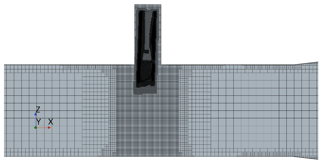
| Property | Mesh |
|---|---|
| Cell type | Trimmed cell |
| 30–50 everywhere | |
| CL number | <10 |
| Physics | Wall function |
| Surface refinement | Around the foil |
| Around the fluid domain | |
| Around the extruder at the top of the tunnel | |
| Around the foil part inside the extruder | |
| Volumetric refinement | Around the foil |
| Around the fluid domain | |
| Behind the foil tip | |
| Number of elements | 7.1 million cells |
| Boundary conditions | Inlet: = 3.26 m/s, defined from |
| A = A to reach | |
| a fully developed flow at the | |
| the foil Position of 9 m/s | |
| Outlet: pressure outlet | |
| Top, bottom, Side, Wall: wall with | |
| no-slip conditions |
| Leeway Angle (T) | Rake Angle (R) |
|---|---|
| 0, 0.3, , | |
| 0, 1, , | |
| 0 | 0, 1, 1.5, , |
| 0.5 | 0, 1, 2, , |
| 1 | 0, 1, 2, 2.5, , |
| 2.5 | 0, 1, 2, 3, 3.75, , |
| 3.5 | 0, 1, 2, 3, 4, 4.75, , |
Publisher’s Note: MDPI stays neutral with regard to jurisdictional claims in published maps and institutional affiliations. |
© 2022 by the authors. Licensee MDPI, Basel, Switzerland. This article is an open access article distributed under the terms and conditions of the Creative Commons Attribution (CC BY) license (https://creativecommons.org/licenses/by/4.0/).
Share and Cite
Marimon Giovannetti, L.; Farousi, A.; Ebbesson, F.; Thollot, A.; Shiri, A.; Eslamdoost, A. Fluid-Structure Interaction of a Foiling Craft. J. Mar. Sci. Eng. 2022, 10, 372. https://doi.org/10.3390/jmse10030372
Marimon Giovannetti L, Farousi A, Ebbesson F, Thollot A, Shiri A, Eslamdoost A. Fluid-Structure Interaction of a Foiling Craft. Journal of Marine Science and Engineering. 2022; 10(3):372. https://doi.org/10.3390/jmse10030372
Chicago/Turabian StyleMarimon Giovannetti, Laura, Ali Farousi, Fabian Ebbesson, Alois Thollot, Alex Shiri, and Arash Eslamdoost. 2022. "Fluid-Structure Interaction of a Foiling Craft" Journal of Marine Science and Engineering 10, no. 3: 372. https://doi.org/10.3390/jmse10030372
APA StyleMarimon Giovannetti, L., Farousi, A., Ebbesson, F., Thollot, A., Shiri, A., & Eslamdoost, A. (2022). Fluid-Structure Interaction of a Foiling Craft. Journal of Marine Science and Engineering, 10(3), 372. https://doi.org/10.3390/jmse10030372