Abstract
The abundance and distribution of marine fishes is influenced by environmental conditions, predator–prey relationships, multispecies interactions, and direct human impacts, such as fishing. The adaptive response of the system depends on its structure and the pathways that link environmental factors to the taxon in question. The “Star Diagram” is a socio-ecological model of marine ecosystems that depicts the general pathways between climate, fish, and fisheries, and their intersection with climate policy and resource management. We illustrate its use by identifying the key factors, pathways and drivers that influence walleye pollock, crab, and sockeye salmon, under a warming scenario on the eastern Bering Sea shelf. This approach predicts that all three species will see reduced populations under a long-term warming scenario. Going forward, the challenge to managers is to balance the magnitude of the effect of harvest and the adaptability of their management system, with the scale and degree of resilience and the behavioral, physiological, or evolutionary adaptation of the ecosystem and its constituents. The Star Diagram provides a novel conceptual construct that managers can use to visualize and integrate the various aspects of the system into a holistic, socio-ecological management framework.
1. Introduction
Variability in the abundance and distribution of marine fishes is influenced by environmental conditions, predator–prey relationships, multispecies interactions and direct human impacts, such as fishing. Although a species can be directly impacted by physical factors (e.g., temperature impact on metabolic rates), the net effect of the various physical and biological factors is the result of complex direct and indirect interactions among them. Fish productivity is, thus, an integrated function within a buffered system, with capacity to absorb the impacts of changing environmental conditions (up to a defined limit, e.g., resilience and tipping points). The way in which the system responds to the environmental and anthropogenic factors depends on the system structure and the nature of the pathways that link environmental factors to the taxon in question [1,2]. Ideally, the response mirrors the scale and re-enforces or complements the type of ecosystem response, without producing negative effects [3]. Once the pathways are better understood and key factors identified, however, the magnitude and type of adaptive response can be better defined and used to devise effective ecosystem-based fisheries management strategies.
Fishery managers generally strive to achieve sustainable/optimum yield, and/or to protect/maintain marine ecosystems. The effectiveness of management strategies in this pursuit is strongly impacted by limitations in gathering and interpreting biological data, inherent environmental variability, and the uncertainty introduced by global climate change [4]. Until we know more about how environmental factors drive the system, and the ways in which these factors interact and will change over time, modifying management strategies to include environmental factors does not improve our ability to achieve management goals much, if at all [4]. The modeling of ecosystem dynamics based on insufficient data leads to uncertainty in model outputs [5]. Szuwalski and Punt [3] noted that in the absence of accurate systems knowledge, management strategies that attempt to account for predicted changes in productivity over time can introduce greater risks if the predicted changes do not occur. Furthermore, different environmental and anthropogenic factors, operating simultaneously, may have complete or partial dominance, be compensatory or interact additively, depending on timing, location, and the state of other associated parameters. It, thus, follows that to support an effective ecosystem-based approach to fisheries management (EBAFM), a key step is to further explicitly define the characteristics of, and interaction among, environmental and anthropogenic factors.
Conceptual ecological models for marine systems that integrate environmental factors, that have direct and indirect influence on commercial fishes, have been developed for the Bering Sea [6,7], the Barents Sea [8], the North Sea [9], amongst others, and described and proposed in general terms [10,11,12]. More recently, conceptual models have more explicitly incorporated anthropogenic effects and drivers for a coastal system in Washington State [13], and the California Current system [14], and there has been a move towards integrated ecosystem assessment models that conceptually also include a diversity of direct and indirect anthropogenic effects on commercial fish populations and their habitat [15]. These approaches vary in their exact configuration but are similar in that they show linkages in a web-like configuration; typically with some weighting of these linkages, sometimes scenario-based. Generally, however, there is little scope for prioritization or bundling of the different parameters, according to their scope, magnitude, scale, and cross parameter linkages.
We propose a new general marine ecosystem conceptual model, in a cyclical framework, that simultaneously captures the hierarchical “cause and effect” relationship among the parameters, while also representing the interconnectedness among them. This new conceptual model allows for incorporation of natural and anthropogenic inputs and helps to effectively identify the most important parameters, their relationships to other parameters, and their synoptic effects across a continuous 360-degree representation of the system. Through the incorporation of the major anthropogenic inputs to the system, our goal here is to apply the model to ecosystem-based fisheries management, related resource management efforts, and research monitoring programs. To avoid a solely abstract representation of our model, we illustrate the general pathways between climate, fishes and fisheries in the Eastern Bering Sea (EBS). We then use this new framework to identify the key factors, pathways and attributes that influence the key commercial species of walleye pollock (Gadus chalcogrammus), crab (including Tanner crab (Chionoecetes bairdi), snow crab (Chionoecetes opilio), blue king crab (Paralithodes platypus), red king crab (Paralithodes camtschaticus)), and sockeye salmon (Oncorhynchus nerka), under a warming scenario on the eastern Bering Sea (EBS) shelf.
2. Conceptual Approach
We propose a conceptual approach called the “Star Diagram” that depicts the linkages between the factors, attributes and drivers of marine ecosystems (Figure 1, Table 1). The overall goal of the Star Diagram is to help illustrate which factors, attributes, and drivers have the potential to affect unique aspects of the species’ life history, and identify through which pathways this influence may occur, so that biological resource management agencies can prioritize monitoring and mechanistic investigation efforts and anticipate how to adaptively respond, going forward into a greenhouse gas- (GHG) driven climate future. We first describe the generic conceptual model and, then, to highlight the relative importance of different pathways with their drivers and factors, we present the application of the Star Diagram for three important fishery taxa in the EBS.
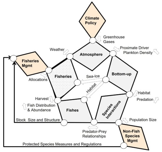
Figure 1.
Star Diagram: Generic conceptual model of a seasonally ice-covered marine ecosystem linking climate policy and resource management to fishes and fisheries. The diagram identifies natural (gray) and anthropogenic (including Fisheries (dotted), and policy/management (orange) Factors (bold labeled polygons that contain specific Attributes listed in Table 1)); Pathways between Factors (circles and arrows), and key Drivers (labels next to Pathways). Arrows indicate the direction in which Drivers act between Factors. See text for further details.

Table 1.
Key Attributes of natural and anthropogenic Factors contained in the Star Diagram conceptual model of a seasonally ice-covered marine ecosystem. Anticipated positive (solid underline) and negative (dotted underline) trends in the values of Climate Policy, Atmosphere and Bottom-up Attributes under a warming scenario in the EBS are indicated (see text for details).
The core of the system is depicted by five linked diamond shaped Factors, labeled in bold (Atmosphere, Bottom-up, Species Interactions, Fishes, Fisheries), forming a pentagon or Star (Figure 1). Each Factor is characterized by a series of Attributes (Table 1). Attributes have interactions (not shown) and some of them mechanistically combine into key Drivers (labels between Factors) that act on other Factors and their Attributes, via a Pathway (circles and arrows). The Drivers can be either basal Attributes, such as temperature, or an integrated measure, such as habitat conditions, and act clockwise, counter clockwise, or be bi-directional (as indicated by arrows). Linked to the core system are three policy/management Factors (Climate Policy, Non-Fish Species Management, and Fisheries Management), which enter the system at different points in the Star Diagram as top-down controls. A more detailed description follows.
Broadly speaking, marine ecosystems are influenced by hemispheric and regional atmospheric Attributes (Atmosphere Factor), such as solar radiation, cloud cover, precipitation, winds, and carbon dioxide (CO2) levels, which are partially determined by a suite of atmospheric greenhouse gases (GHG Driver), such as carbon dioxide and methane, that are regulated by national and international climate policies (Climate Policy Factor). The Atmosphere Factor has a far reaching and deeply penetrant influence and has, thus, been deliberately placed at the most prominent position, in the core of the Star Diagram. Atmosphere Attributes culminate in four Proximate Drivers (air temperature, wind, CO2 levels, and light intensity) that propagate through the system in a clockwise fashion, via the Pathway from Atmosphere to the Bottom-up Factor. These four Proximate Drivers, by themselves and/or in combination, largely determine the temporal and spatial characteristics of the physical and chemical Attributes of the Bottom-up Factor. The physical and chemical Bottom-up Attributes interact with each other to influence biological Bottom-up Attributes, such as production, abundance, phenology and species composition of ice algae, heterotrophic microbes (phytoplankton), zooplankton, ichthyoplankton and forage fishes. Atmosphere and Bottom-up Attributes in Table 1 are shown in solid underline or dotted underline, depending on whether they are predicted to decrease or increase during a warming scenario. The influence of, and interactions among, Bottom-up Attributes to specific fish species are the subject of the application of the Star Diagram, as detailed in the three case-studies below.
There are three different Bottom-up Drivers that influence other parts of the system through four Pathways, as follows: plankton Density, which feeds back to influence the solar radiation attribute, as it impacts light intensity in the water column, and the CO2 levels attribute, via a reduction in water column mineral carbon (Ortiz et al., 2016); sea ice timing and extent, which influences the Fisheries Factor because the presence of ice can limit access to certain fishing areas [16]; habitat, defined as an aggregate of three key single or composite Attributes (water temperature, ocean pH, and prey), which influences Fishes Factor Attributes directly, but also indirectly, through the Species Interactions Factor, by determining the extent of spatial and temporal overlap among fishes, seabirds and marine mammals affecting predation (including cannibalism) and competition (predator–prey relationships). The Species Interactions Factor is further influenced by management decisions affecting seabirds and marine mammals, as captured by the Non-Fish Species Management Factor, by impacting the Driver Population Size of key fish predators and competitors, which, in turn, also feeds back to the biological Bottom-up Attributes.
In addition to habitat and predator–prey relationship drivers, the Fishes Factor is impacted top-down, through Harvest pressure from commercial and subsistence Fisheries. In turn, the Distribution and Abundance of Fishes Drivers provide feedback to Fisheries by influencing real-time decisions made by fishers about where and when to fish (defined as harvester behavior in [17]. In combination, the three Pathways modifying Fishes Factor Attributes, result in a fish Stock Size and Structure Driver that is assessed through systematic surveys and directly influences Fisheries Management decisions, such as catch limits, different harvest control rules, area closures, and other ecosystem conservation measures (e.g., EBAFM, Fishery Ecosystem Plan—FEP). Fisheries Management decisions may also be directly influenced by management decisions made for Protected Species, such as those which, in the U.S., would come through the Endangered Species Act (ESA), or the Marine Mammal Protected Act (MMPA). Specific fisheries Allocations decided in this manner then circle back to the Fisheries Factor and influences its key Attributes, such as Fleet Size and Composition, Quotas, Seasonal Distribution of effort, etc. It is at this juncture that we come full circle, and allocated fishery effort is influenced by sea ice, as previously noted, and the Weather Driver (particularly the occurrence and severity of storms), via the Atmosphere Factor.
The Star Diagram identifies the different system Factors, Attributes, Pathways and Drivers that structure marine ecosystems, but does not mean to imply that these characteristics are consistent in time or space, e.g., [18] or that all are of the same relevance to all species. Indeed, temporal and spatial variation is at the heart of the difficulty in elucidating the complexity of marine ecosystems and setting sustainable and adaptable policies that properly account for habitat, species management, their interactions, and other ecosystem services. The effect of each of the constituents of the Star Diagram will vary in intensity and direction of influence, not only intrinsically, but also depending on the degree and type of interaction among them, whether additive, compensatory or neutral, and the physiological needs of particular taxa (Figure 2).
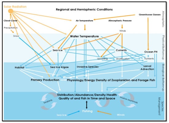
Figure 2.
Interactions within and between Atmosphere and Bottom-up Factors influencing Fish and Fisheries (example includes sea ice for application to marine ecosystems impacted by seasonal ice).
To illustrate the utility of the Star Diagram, we present three case studies from the Eastern Bering Sea (EBS), where the North Pacific Fishery Management Council (NPFMC, one of eight U.S. regional councils established by the Magnuson–Stevens Fishery Conservation and Management Act in 1976 to manage fisheries in the 200-mile Exclusive Economic Zone) is implementing a Fishery Ecosystem Plan (FEP) to help further EBAFM for the Bering Sea, where a lot of new understanding has been gained by ecosystem level research, conducted over the last decade (described in [19], and extensively published in [20,21,22,23]. The purpose of FEPs is to provide fishery management councils with a foundation from which to apply a comprehensive understanding of the habitat and biology of species, fishery information, social and economic impacts of management actions, and the ecological consequences of conservation and management strategies [24]. As such, a major task for the design of FEPs is to describe the current state of the science, regarding ecosystem structure and function, and to establish how fisheries impact, and are impacted by, the broader ecosystem in which they operate. Here, we first provide a general characterization of the EBS marine ecosystem and describe the regional Driver status and trends of the Atmosphere and Bottom-up Factors that define habitat for fishes, birds, and marine mammals. From this foundation, we apply the Star Diagram conceptual model to three specific case studies on walleye pollock, crab (multiple taxa) and sockeye salmon, with the ultimate goal of clarifying how climate-driven change will alter distribution, abundance, health and survival of these important taxa, and thus, highlight what managers and policy makers should focus on to monitor and sustainably manage this complex system.
3. Eastern Bering Sea
The eastern Bering Sea marine ecosystem supports fisheries that provide almost half of all seafood consumed in the United States [25,26]. The EBS consists of a broad (~500 km) shelf, extending approximately 1000 km from the Alaska Peninsula, north to the Bering Strait [27]. The shelf slopes gently from the coast, westward to the shelf break at about 180 m depth (Figure 3). South of 62° N, patterns of wind and tidal energy divide the shelf into the following three cross-shelf domains during spring, summer, and fall [28,29,30]: the coastal domain (<50 m water depth), which is vertically well-mixed by tidal and wind mixing; the middle shelf domain (~50–100 m), which is sharply stratified into an upper mixed layer, and a lower mixed layer; the outer shelf domain (~100–180 m), where the surface wind-mixed layer and the bottom tidally mixed layer are separated by a transitional layer. Each of the regions has its own chemical signature [31,32], biological communities, and levels of lower trophic-level production [33,34,35,36,37,38]. Numerous physical and biological connections have been identified between the different physical domains, e.g., [6,39,40].
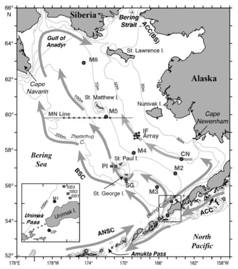
Figure 3.
Eastern Bering Sea study area showing major isobaths. Currents, place names and mooring sites (circles and squares, e.g., IF, CN, M2). “X” indicates hydrographic stations. UP is Unimak Pass, SB is Slime Bank, SG is St. George Island, PI is the Pribilof Islands, IF is the inner front. (Figure reproduced from [41], with permission from Elsevier as per STM guidelines).
The Bering Slope Current (BSC) is a major source of transport that influences conditions on the inner and middle Bering Shelf domains. Largely fueled by the Aleutian North Slope Current (ANSC), the BSC has either an ill-defined variable flow, interspersed with eddies and meanders [42,43], or a more regular, northwestward flowing current [44,45]. Exchange across the shelf break is likely dependent on which of these two flow patterns are dominant. The BSC is important due to its transport of heat and nutrients, but it also transports the eggs and larvae of several demersal fish species, such as Walleye Pollock [46], Greenland (Reinhardtius hippoglossoides) and Pacific halibut (Hippoglossus stenolepis) [47], and other flat fishes [48], from the oceanic and slope region to the Outer Shelf Domain, where the habitat is more conducive to result in higher survival rates. The on-shelf flow mode of the BSC varies as a result of wind-driven advection and interaction of the BSC with bathymetry, in particular, the funneling effect of canyons [38,49,50,51,52].
Sea ice is a prominent feature of this northern sea and is a critical component of the physical oceanography of the Bering Sea Shelf, which structures the spring habitat, impacts the phenology of primary and secondary production, and provides a breeding and resting platform for birds and seals, as well as hunting and traveling platforms for coastal communities, e.g., [53,54]. The timing and fate of the primary production has dramatic consequences for both benthic and pelagic organisms [54,55]. During fall and winter, nutrient levels on the shelf are replenished, at least in part, from the Bering Sea Basin. When the sea ice melts in the spring, nutrients from sediment, trapped in the ice, are released, contributing to primary production. Ice algae production begins prior to ice melt and the stratification that leads to the primary spring bloom typically begins to set up in May and breaks down in September/October; these dates can vary by more than 30 days [56]. In the northern Bering Sea, the majority of the primary production is not consumed in the water column, and eventually sinks to the sea floor to be consumed by benthic epi- and in-fauna, making the ecology of the northern Bering Sea Shelf predominantly benthic [6,57,58,59]; cited by [30]. As a result, benthic feeders, such as walrus, spectacled eiders and gray whales, are predictively found on the northern shelf in abundance, depending on the time of year. In the southern Bering Sea, light and nutrient levels are such that grazing zooplankton can take advantage of the primary production in spring and summer, supporting pelagic fishes (e.g., pollock), sea birds (e.g., short-tailed shearwaters, and crested and least auklets) and baleen whales, such as fin and humpback.
3.1. Driver Status and Trends
3.1.1. Proximate Drivers
Large scale atmospheric patterns, such as the Arctic Oscillation (AO; [60]), the Aleutian Low (AL; [61]), and Pacific Decadal Oscillation (PDO; [62]), are influenced by greenhouse gases (GHGs; predominantly carbon dioxide, methane and nitrous oxide) and impact air temperature, winds, cloud cover, and precipitation (Figure 2). Based on the trends and patterns of these larger scale drivers, and predicted increases in GHGs by 10–25% from current levels by 2030 [63,64], it is anticipated that the climate in the southeastern Bering Sea, over the next few decades, will continue to be dominated by a progression of warm and cold fluctuations of interannual, or longer, intervals, arising intrinsically [65], with a long-term overall warming trend [66]. Greenhouse gas-driven warming will warm the Arctic much faster than more temperate regions [67], and is predicted to reach an average rate of change of 0.6 °C per decade by the year 2020 [68]. This trend will also drive increased freshwater input into the Bering Sea via accelerated glacial ice melt [69].
Cloud cover [70] and precipitation [71] in the EBS and adjacent areas are projected to increase by 15% to 30%, across all four seasons by late this century [72,73]. Precipitation in the form of snow falling on sea ice has particularly potent effects on marine ecology, because it acts as an insulating blanket, slowing down air-driven ice melt and reducing photosynthetically active radiation (PAR) penetration into the water column. Snow cover also provides important denning habitat for polar bears and ringed seals [74,75]. Warming air temperatures are increasingly turning snow to rain and have led to a decline of snow cover in the Northern Hemisphere by about 10 percent since the late 1960s, with stronger trends noted since the late 1980s [76]. In Alaska, the snow cover duration dropped by 15 days from 1980 to 2009, with a significant decrease in snow cover extent, particularly in spring, with a 4 to 6 day earlier disappearance of snow [76]. As a result, the 40-year record on solar heating shows a long-term increasing trend and reduced surface latent-heat fluxes, correlated with increases in sea surface temperatures [77].
Surface winds have a strong effect on the marine ecology of the Bering Sea, by promoting mixing [56], driving transport of zooplankton, phytoplankton, heat [78] and sea ice [45], all of which are closely tied to pelagic-benthic coupling and production and provision of prey for larval fish [79]. Surface winds arise due to spatial differences in surface pressure, which in the Bering Sea, are dominated by the location of the Aleutian Low (AL) [45,61]. Models predict that under warming conditions, the AL will move northward, resulting in an increase in the predominance of southwesterly winds in spring and increased westerly winds in fall, but with weaker winds overall, especially northeasterly [27,80]. A relative increase in southerly winds (generally warmer than northerly) will promote a decrease in the extent of sea ice [27] and result in the greater on-shelf transport of salty, nutrient-rich waters across the shelf break [81].
3.1.2. Plankton Density
The overall effect of climate change on Bering Sea phytoplankton community composition, biomass and rates of production is difficult to predict. Multiple parameters, such as ice thickness, snow cover, cloud cover, winds, and nutrient availability, shape primary production, whether it be associated with ice, or in the surface or sub-surface water [82]. Predicted decreases in snow cover, with an associated increase in light penetration through the ice, would result in increased ice algal production if nutrients are present to support it. However, a reduction in maximum sea ice extent and earlier sea ice retreat will likely overrule the effect of reduced snow cover and lead to a net reduction in ice algal production, with less availability of this important food source in winter and spring, particularly on the far southern reaches of the shelf [83]. Warmer temperatures appear to lead to higher water column phytoplankton production [84,85]. Years with significant ice after mid-March generally see an early (March–April) pelagic bloom, accompanied, during some years, by a second bloom in May or June, resulting from an injection of bioavailable nitrogen into the upper-water column [86]. This does not necessarily suggest, however, that warm years, which may only have one spring bloom, cause an overall decline in total annual production; some evidence suggests that spring bloom magnitude may be higher overall when ice and ice algae are absent [86]. Likewise, Eisner et al. [87] found that late summer and early fall chlorophyll a values were higher during warm years. Taken together, a future warmer Bering Sea may have increased overall primary production, with a concomitant decline in ice algae production.
3.1.3. Sea Ice
The thickness, areal coverage, and southern extent of sea ice vary on multiple timescales [27,88,89,90]. Examination of the patterns of sea ice formation and retreat shows that there is always ice on the northern Bering Sea shelf (north of 60° N) during winter and much of spring, with the variability occurring predominantly in the south [27]. Sea ice extent in March and April determines the temperature and extent of the Bering Shelf cold pool of the middle shelf of the southern Bering Sea [27]. Climate models suggest large declines in sea ice extent in the Alaskan region [65]. A decrease in the southerly extent of sea ice, coupled with an earlier retreat, will result in an increase in temperature and a reduction in size of the cold pool throughout the south [58,91]. Modeling carried out by Wang et al. [92] predicts complete loss of summer sea ice in the Chukchi Sea, between 2030 and 2050, and areal losses of winter sea ice in the Bering and Chukchi seas of more than 50% by the end of the century. Cheng et al. [91] predicts a northward shift of ice extent by ~2° latitude in the next 40 years. Such changes in the sea ice will have particularly strong effects in the south, by delaying the timing of primary production and impacting the distribution and species composition of primary and secondary producers. Indeed, projections for future SST anomalies for the Bering Sea show an increase in frequency of positive anomalies for all months, which tracks the predicted increases in air temperatures described above. The decreasing sea ice coverage, combined with overall weaker winds [27,80], is expected to lead to stronger upper layer stratification in springtime, with associated decreased nutrient availability in surface waters [93], which would shift the system towards a late spring bloom initiation [80]. This will, in turn, have effects on production of the commercial fishery species, such as pollock, cod, salmon and crab [27,40,54,58,94].
3.1.4. Habitat
Water temperature, pH, prey abundance, and prey nutritional value combine to make up the key aspects of habitat for fishes, birds and mammals. The Bering Sea goes through cycles of cold and warm periods, with the latest cooling trend stretching from 2005 to 2011 [27], but with an apparent warming trend beginning in 2013 [41]. Climate-driven simulations, for over the next several decades, suggest a warming of 1 to 2 °C but still with considerable uncertainty in the interannual and interdecadal variation between the models [95]. The projection in Herman et al. [95] suggests that there will be less ice on the southern shelf, but ice will continue to form in the northern Bering Sea in the winter up to 2040. Spatial (both horizontal and vertical) and temporal heterogeneity in the projected warming is less predictable than projections across the entire system.
The ocean has absorbed more than 25% of the total anthropogenic-derived CO2, resulting in a global surface ocean pH decrease of approximately 0.1 units [96,97], rendering the ocean 30% more acidic today compared to pre-industrial times [98]. More rapid and seasonally intensified decreases in pH have occurred in the Bering Sea, in part due to freshwater runoff and changes in benthic-pelagic coupling, leading to increased remineralization [99,100,101]. The decline in pH can have direct effects on various species by lowering the concentration of carbonate, which is essential for the growth and maintenance of crustaceans, mollusks and corals, and can also affect many species indirectly, by reducing the abundance, distribution and energy content of their prey [98,102]. Important effectors of ocean pH in the Bering Sea, besides atmospheric CO2, are phytoplankton production, freshwater runoff, timing and extent of sea ice and remineralization of organic carbon. Under a warming scenario, the only one of these effectors that serves to curb acidification is the anticipated increase in upper ocean primary production in summer. All the others are anticipated to lead to increased ocean acidification in surface and bottom waters in spring and summer [99,100,101].
Zooplankton, ichthyoplankton, and forage fishes combine to make up the key prey for fishes, birds, and mammals. Zooplankton abundance, distribution and community composition can change dramatically in the Bering Sea, due to the interaction of wind and ocean circulation; these drivers determine which zooplankton species that over winter off-shelf make it on to the shelf in the spring. Ice dynamics drive the type and amount of food that is available to zooplankters on the shelf once they arrive there [27]. Under warming conditions, as substantiated by past warm periods, there is likely to be lower large crustacean zooplankton abundance and biomass [87,103], due to decreased winter survival, caused by a reduction in fat storage, a decrease in ice-algae, a shift in phytoplankton community composition and phenology [84], increased respiration due to warmer temperatures [83,85,86], and increased predation [86,104]. Abundance of small taxa and gelatinous zooplankton, however, is predicted to increase due to more growth-favorable temperatures, increased food availability, and production of more cohorts during a longer growing season [87,105].
Ichthyoplankton community-level responses to a warming southeastern Bering Sea show strong spatial patterns, related to water column temperature, salinity, cross-shelf transport mechanisms [104,106], and developmental stage [107]. Each species will react in different ways, although, in general, larval abundances have been observed to be greater in warm years [106].
Species and location-specific responses to warming are expected for forage fish, such as capelin (Mallotus villosus), sandlance (Ammodytes hexapterus), herring (Clupea pallasii) and early life stages of commercially important species [108,109,110]. Their responses are directly impacted by temperature preferences, and indirectly through the effect of a warmer ocean on their prey [111,112]. For example, as large zooplankton decline during warm years, fewer age-0 walleye pollock survive their first winter, causing concern for other fishes, including salmon, herring, and capelin that turn to age-0 pollock as prey, when large zooplankton are not available [13,112]. In addition, without large zooplankton to eat, the bigger of the age-0 pollock appear to consume the smaller age-0 pollock individuals, thus, further lowering pollock population size. Observations suggest that a reduction in large lipid-rich crustacean zooplankton, leading to increased predation pressure on forage fishes, is at the center of an overall system-wide decline in forage fish abundance in a warming scenario.
Biotic impacts of the projected changes in the sea ice and habitat driver attributes are species-specific, depending on physiological preferences, nutritional requirements and adaptability. Because these drivers also influence temporal and spatial overlap between predators and prey [113,114,115,116,117,118], they also impact dynamics governing Species Interactions and Predator–Prey Relationships. We present three case studies to illustrate to what degree, and through which Pathways, these biotic and abiotic Drivers may affect Fishes Attributes. We examine the implications of these findings for ecosystem monitoring efforts and fishery management in the discussion.
4. Case Studies
4.1. Case Study 1: Walleye Pollock
We focus on Walleye Pollock as one of the focal species because it supports the largest single species fishery in the Bering Sea, is arguably the best studied species in this system, provides insight into the mechanisms driving the pelagic food web, and is a species with a moderate to warm temperature preference.
4.1.1. Habitat and Sea Ice
The Bottom-up Attributes, pH, water temperature, and prey field combine to characterize Habitat for walleye pollock. Examination of Bering Sea physics and biota in the recent warm (2001–2005) and cold (2007–2010) phases has provided a natural laboratory for assessment of the potential effects of climate warming. Experiments indicate that hatching and early growth of walleye pollock are not negatively affected by CO2 levels, even in excess of those predicted under warming climate scenarios [119], and there is no evidence to suggest that pollock of the later life stages are directly affected either [120]. Thus, marine fishes with high metabolic rates and well-developed acid-base regulatory systems, such as pollock, are believed to have the capacity to adapt to reduced pH levels [121,122]. Indirectly, however, there are potential concerns about the effects of ocean acidification on abundance, health, and species composition of their preferred invertebrate prey, such as copepods and euphausiids [123]. Although we have little predictive ability on the response of zooplankton populations to ocean acidification [124], recent findings from the Pacific coast of North America indicate that euphausiids, and potentially other zooplankton species that experience a range of pCO2 values during diel migration, have high adaptability to reduced pH levels [125].
Warmer water temperatures appear to directly increase the growth of walleye pollock at early stages and increase metabolic rate [126]. Caloric requirements of adult pollock are projected to increase by 26%, with a rise in water temperatures of 2 °C [127]. The direct effects of increased caloric requirements are exacerbated indirectly by lower numbers of large lipid-rich copepods and euphausiids on the shelf during warmer water conditions [27,54,87,108,128]. This leads to reduced lipid storage of young pollock in the fall, and a decrease in over-winter survival [27,129,130,131]. The effect of low lipid storage before the onset of winter is exacerbated by a delay in the production cycle the following winter/spring (i.e., late spring bloom due to early sea ice retreat and reduced ice algae production), making the period without sufficient prey resources even longer [131]. Warm water conditions expand the habitat for adult pollock [116], which leads to greater spatial overlap between adult and young pollock, and a spatial mismatch between age-0 pollock and their preferred prey [126]. An overall reduction in the preferred prey, large lipid-rich zooplankters, results in increased cannibalism of 1+ pollock on their age-0 con-specifics, and as mentioned previously, of larger age-0 pollock on the smaller age-0 pollock [132]. Warmer water conditions also lead to a spatial and temporal reduction in sea ice, affecting fishing effort, although there is still much uncertainty about future fishing conditions, and annual variation in ocean temperatures and economic factors has, thus far, been more significant than long-term climate change-related shifts in the fishery’s distribution of effort [17]. Nevertheless, this study found that warm temperatures and high abundances lead to more intense harvesting of earlier-maturing roe in winter, whereas in summer, warmer ocean temperatures were associated with lower catch rates. Production-related spatial price differences affected the effort distribution by a similar magnitude.
4.1.2. Predator–Prey Relationships
Species interactions leading to predation on pollock by other taxa (i.e., other fishes, seabirds and marine mammals) is a significant factor in the control of production of the fishable pollock population. Disparity in the responses of pollock and their predators to changing ocean conditions can potentially lead to a climate-driven increase in the relative impact that predators may have. For example, arrowtooth flounder, a predator of young pollock, do not appear to be affected by warming water temperatures [27], but the expanded warm water habitat for pollock has been shown to increase the habitat overlap between pollock and arrowtooth flounder, leading to anticipated increased predation pressure on age-1 pollock in the coming decades [133]. Similarly, warming conditions in the short term appear to promote higher recruitment of sockeye salmon (see sockeye salmon section below), that in turn switch preferentially to age-0 pollock prey, with the aforementioned reduction of larger lipid-rich zooplankton, resulting in further potential increases in predation [134].
Other predators whose population size and distribution may be affected by climate change with related effects on pollock, include flat head sole (Hippoglossoides elassodon), the surface-feeding black-legged kittiwake (Rissa tridactyla), the diving thick-billed murre (Uria lomvia), humpback whale (Megaptera novaeangliae), fin whale (Balaenoptera physalus), sea lion (Eumetopias jubatus), and fur seal (Callorhinus ursinus) [114,135,136,137]. However, there is still a general lack of research similar to that of Hunsicker et al. [133], that empirically address how climate-driven responses of these taxa in the Eastern Bering Sea will affect co-localization and predation on pollock.
4.1.3. Summary of Relevant Effects of a Warming Bering Sea on Pollock
A warmer Bering Sea leads to larger area of preferred thermal habitat, increased productive output, and higher early growth rates. However, it also creates a decrease in the preferred large lipid-rich zooplankters and to increased predation by older pollock, arrowtooth flounder and sockeye salmon. The net effect is a decrease in habitat quality for pollock, leading to insufficient lipid storage of early pollock life stages and decrease winter survival. Ultimately, despite a higher number of young early on, these factors lead to fewer adult pollock and a decrease in the fishable population and commensurate allocations (Figure 4). The way in which other pollock predators will respond to climate change with associated effects on predation has not been determined at a sufficient level of detail to ascertain their effects on pollock. Our examination on the potential effects of different biological, physical and chemical parameters, through the Star Diagram, qualitatively concurs with the overall prediction of Mueter et al. [130], who estimated a decline in pollock recruitment of 32–58% by 2050, assuming an increasing warming trend in the Bering Sea. The direct fisheries management and fisheries Attributes and Drivers impacted by this decline would be fishing allocations and quotas, which could be used to reduce the harvest, and thus, attempt to minimize additional anthropogenic stressors on this population.
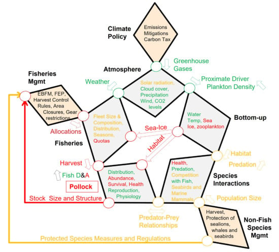
Figure 4.
Attributes, drivers and pathways affecting pollock population dynamics in the EBS. Red (negative), green (positive), yellow (neutral or unknown) text or lines are used to indicate the directionality of the attribute, driver or pathway in a warming scenario. Black text refers to example attributes that can be modified through direct policy or management actions. See text for details.
4.2. Case Study 2: Crab
Our second example focuses on commercially exploited benthic crab species in the Bering Sea, including Tanner crab (Chionoecetes bairdi), snow crab (Chionoecetes opilio), blue king crab (Paralithodes platypus), and red king crab (Paralithodes camtschaticus). Crab currently and historically support a significant commercial fishery in the Bering Sea. As a group, they show a cold to moderate temperature preference and an examination of climate pathways leading to crab provides insight into the mechanisms impacting the benthic food web.
4.2.1. Habitat and Sea Ice
The Bottom-up Attributes, pH, water temperature, ice algae, and phytoplankton and zooplankton abundance and distribution, combine to directly or indirectly influence Habitat quality for crabs in the EBS. Laboratory studies have shown that decreasing the pH of bottom water can potentially have direct deleterious effects on crab physiology and habitat suitability. The work of Swiney et al. [138] and Long et al. [139] on Tanner crab, show that treatment at low pH 7.5 (ambient is typically 8.1), during development, had negative effects on morphology, size, metabolic rate and Ca/Mg ratio, with a 71% reduction in hatching success. In addition, developing females had softer carapaces with reduced Ca content. Similarly, Sigler et al. [140] showed lower survival, growth, and Ca content in king crab when exposed to low pH water. Both red king crab and Tanner crab have exhibited slowed growth and decreased molting success in waters with a pH of 7.8, and crabs died in more acidified conditions (pH = 7.5) [141]. Individual level variation in tolerance to low pH has been found [138,139], suggesting that existing genetic variability may underlie tolerance or greater phenotypic plasticity that may allow for adaptation to more acidic bottom water. The range of adaptability and effectiveness of natural selection in promoting pH tolerance are not known. In addition to these laboratory studies, modeling results by Punt et al. [142] predicted declines in the yields from red king crab fishery over the next 50 to 100 years, driven by reduced pre-recruit survival due to increased Ocean Acidification (OA). Reducing pH can also affect calcifying organisms that are prey for crab, potentially further contributing to the overall negative effect of acidified bottom water. Despite laboratory findings and model predictions, the effects of reduced pH on crab populations have yet to be documented in the field.
Water temperature along the ocean floor is a prime determinant of crab habitat [116,143,144]. There is a positive relationship between temperature and red king crab growth [145], and Tanner crab that settle in warm waters mature more quickly [146]. Faster growth and maturity of crabs, however, may not translate into higher recruitment of mature crabs into the fishery. Synoptic effects of a warmer Bering Sea, such as delayed and reduced export of carbon to the benthos (late spring bloom due to early sea ice retreat and reduced ice algae production), may create a mismatch between crab metabolic requirements coming out of the winter season and provisioning through primary production and benthic export. Benthic community composition and productivity are primarily a function of substrate, temperature and the quality and quantity of primary production (ice algae and phytoplankton) that settles to the bottom. As discussed, conditions in a warming Bering Sea generally lead to later spring bloom initiation that favors the routing of reduced carbon to the zooplankton [147]. On one hand, this tends to prevent a lowering of the pH of bottom water through re-mineralization, while on the other, it may reduce the production of benthic organisms, including crab and their prey [101]. Bottom water temperature also delineates preferential habitat, with the 1 °C isotherm most commonly affecting spatial distribution of crab [116]. Expansion of the cold pool (bottom water fingerprint, left behind by the winter sea ice extent) during the cold phases in the Bering Sea, for example, drives a more southerly distribution of C. opilo [116]. However, this sub-decadal scale pattern is embedded in a general northward expansion in distribution of crab over the last 30 years [94]. The general northward “expansion” seems to be a combined effect from commercial harvest, increasing temperature, and reductions in sea ice in the south [94].
4.2.2. Predator–Prey Relationships
Red king crab, Tanner and snow crab larvae are planktonic feeders and consume both phytoplankton and zooplankton, including diatoms, algae and copepods [148,149]. During this stage, their diet overlaps with that of forage fish which, overall, are predicted to decrease in warming years [13,112]. A warming Bering Sea could, therefore, lead to increased phytoplankton and zooplankton prey for crab larvae. At the juvenile and adult stage, crab are opportunistic, omnivorous benthic scavengers, who compete with other benthic foragers, such as flatfish and skates, for food [150], who also consume crab [151]. A range of predators prey on crab during all but the adult life stage and include marine mammals (seals and sea otters), seabirds, octopus, and a range of fish species [6,152,153,154,155]. Pacific cod (Gadus macrocephalus), in particular, has been suggested as a major controller of crab recruitment [155], with the ability to remove up to 94% of age-1 Tanner crab and up to 57% of snow crab in the Bering Sea in a single year [156]. Over the last thirty years, however, an increase in tanner and snow crab mature male biomass, from the EBS trawl survey, is evident, with a decrease in the Pacific cod biomass. In turn, increasing Pacific cod and yellowfin sole biomass have been associated with declining Bristol Bay red king crab recruitment [152,153]. Ultimately, the net result of changes in predation upon the commercial crab species in a warming Bering Sea remains difficult to predict, particularly as both crab and their predators undergo changes in their temporal and spatial distributions and southern species are moving into the region.
4.2.3. Summary of Relevant Effects of a Warming Bering Sea on Crab
A warmer Bering Sea leads to a constriction of preferred thermal habitat for juvenile and adult crab to the north, and decreased export of ice algae, phytoplankton, and zooplankton to the benthos, in many parts of their current distribution. Increased freshwater run-off, increased absorption of carbon at the ocean surface due to overall increased primary production, and increased remineralization, all combine to increase the acidity of bottom waters, further impacting habitat quality and physiology. Together, these attributes and drivers are expected to lead to a smaller spatial distribution, decreased survival, and decreased overall abundance of adult crab, with commensurate reductions in harvest allocations (Figure 5). What the net result of changes in species interactions will be on crab populations under this scenario is unclear, as is the knowledge as to how far the storehouse of genetic variation and phenotypic plasticity can be extended to adapt to the new conditions. A decrease in crab distribution and abundance, and associated uncertainties, could lead to a decrease in the spatial distribution of the fishery. Fisheries and Fisheries Management responses to these changes and uncertainties could be modifications in allocations, quotas and harvest, which could lead to a reduction in fleet size, but also help to minimize additional anthropogenic stressors on this population.
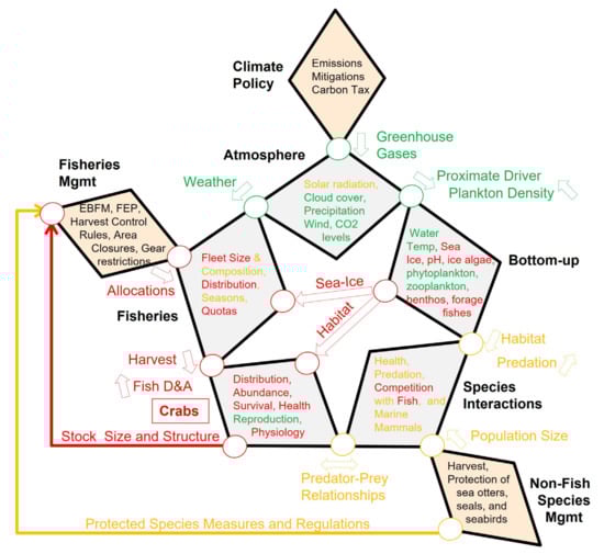
Figure 5.
Attributes, drivers and pathways affecting crab population dynamics in the EBS. Red (negative), green (positive), yellow (neutral or unknown) text or lines are used to indicate the directionality of the attribute, driver or pathway in a warming scenario. Black text refers to example attributes that can be modified through direct policy or management actions. See text for details.
4.3. Case Study 3: Sockeye Salmon
Sockeye salmon is the third species we use to illustrate the effects of, and interactions among, the drivers that will shape the marine ecosystems in the Bering Sea under a warming scenario. Salmon in general, and Bristol Bay sockeye salmon, in particular, is the most valuable commercial fishery managed by the State of Alaska, and key to a traditional subsistence lifestyle in the region (http://www.adfg.alaska.gov/index.cfm?adfg=fishingcommercialbyfishery.main, accessed on 6 November 2021). Sockeye salmon is an anadromous species, typically spending their first year in freshwater lakes. We focus on the marine portion of sockeye salmon life history; climate driven change on the freshwater aspects have been well covered in the literature, particularly with regard to potential temperature effects (see [157] for a synthesis).
4.3.1. Habitat
Warming water may directly affect sockeye salmon physiology and habitat suitability and, in addition to a decreasing pH, also have indirect effects via impacts on prey and predator abundance and distribution. It appears unlikely that ocean acidification, at least over the short term, will have strong direct effects on sockeye salmon, but it may have significant deleterious effects on sockeye prey, in particular, the shelled pteropod Limicina limicina, thought to be important prey for juvenile salmon in Alaskan waters [158,159]. Although there is no current evidence of declines in pteropod abundance in the Bering Sea, such declines have been noted in British Columbia [160] and the Southern Ocean [161], and lab studies clearly show deleterious effects of low pH on pteropods [162]. Whether a potential future decline in pteropod biomass in the Bering Sea manifests and would impact recruitment of sockeye will depend on the availability of other taxa that could potentially function as substitute prey.
Direct effects of temperature on sockeye salmon include effects on metabolism, growth, and phenology. While warmer than average seas have been linked to increased juvenile sockeye salmon abundance and growth during the open-ocean phase [163], warmer water during the last months of ocean residence has been related to small body size and lower energy levels at maturity [164,165,166]. Increased survival was noted for Alaskan sockeye salmon when ocean temperatures are cooler two months prior to spawning migration [167]. Reduced growth and energy levels exhibited by BC sockeye salmon experiencing warm conditions towards the end of their ocean residence, a critical period when they acquire 50% of their final mature body mass [168], likely resulted from increased metabolic rates [169,170], combined with decreased availability and limited distribution of food [158,171,172]. Mueter et al., [173] showed that warmer coastal conditions were correlated with increased survival of Alaskan sockeye salmon populations. The decreased survival of sockeye salmon from British Columbia and Washington under warm conditions suggests that the southern populations may be closer to the temperature-driven tipping point than the more northern populations.
The indirect effects of temperature are various, with prey type and availability central among them. Prey type and availability affects growth rate (size) and ability to store lipid (energy density). Size-dependent mortality is an important selective process for juvenile sockeye, with larger individuals faring better [174,175]. Overwintering survival in marine waters also appears to be a critical selective period, with energy density positively related to winter survival [176]. In cold years, juveniles feed on lipid-rich euphausiids and copepods. In warm years, production of copepods and euphausiids declines and juvenile sockeye feed increasingly on age-0 walleye pollock [134], which have lower energy density than the preferred crustacean prey. The high marine survival of juvenile sockeye in warm years appears to be promoted by an increase in pelagic production that compensates for a relative reduction in lipid-rich crustacean prey and increased metabolic demand. Too large an increase in temperatures past a tipping point, however, may disrupt this net positive balance [166], resulting in lowered marine survival of sockeye and their alternate warm water prey. For instance, walleye pollock do worse under the approximately 1 °C warmer conditions under which sockeye thrive [163], and Abdul-Aziz et al. [177] estimated a 38% decrease in sockeye winter habitat by the middle to late 21st century.
4.3.2. Predator–Prey Relationships
Sockeye are subject to predation at all life history stages [178] and compete with other taxa (particularly other salmonids) for niche space. In the early marine phase, predators include beluga whale, seal and porpoise, diving birds and chinook and coho salmon [179]. During the open ocean phase, they are preyed upon by a series of pelagic fish species, as well as by sharks and marine mammals [180,181]. Okey et al. [182] presented information on the potential effects of the climate-driven distribution shift of salmon sharks, but for most predators of sockeye salmon, there is relatively little understanding of how climate-driven changes will affect predation. More information is available on competition. Populations of pink salmon in the Bering Sea have increased over the past decades [183], putting pressure on sockeye. High pink salmon abundance during the second year of sockeye ocean residence, for example, was shown to reduce sockeye recruitment [184,185]. Whether or not the atmospherically driven changes in the eastern Bering Sea promote pink over sockeye is not known, although pink salmon are known to have a wide physiological tolerance, which may allow them to thrive with attendant negative impacts on sockeye salmon in a warmer Bering Sea [186].
4.3.3. Summary of Relevant Effects of a Warming Bering Sea on Sockeye Salmon
Over the short term (<10 years), the aggregate direct and indirect effects of relatively warm spring conditions in the Bering Sea are anticipated to lead to higher winter survival of juvenile sockeye, due to higher pelagic productivity and increased growth rate [163,187,188]. Over the long term (>10 years), however, warming seas combined with potential reductions in important food items (e.g., shelled pteropods) and increased competition suggest that the future of sockeye salmon in the Bering Sea may be under threat [177], Figure 6. Predation effects can be substantial on sockeye populations, but there remain too many uncertainties around whether this top-down pressure and intra and inter-specific interactions will be net positive or negative. The direct fisheries management and fisheries Attributes and Drivers impacted by this decline would be fishing allocations and quotas, which could be used to reduce the harvest and, thus, attempt to minimize additional anthropogenic stressors on this population.
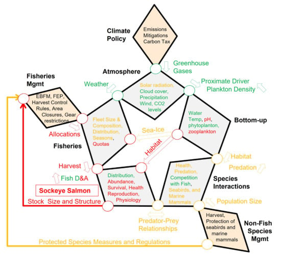
Figure 6.
Attributes, drivers and pathways affecting sockeye salmon population dynamics in the EBS. Red (negative), green (positive), yellow (neutral or unknown) text or lines are used to indicate the directionality of the attribute, driver or pathway in a warming scenario. Black text refers to example attributes that can be modified through direct policy or management actions. See text for details.
5. Discussion and Conclusions
The combination of continued external forcing by anthropogenic GHGs, the residence time of GHGs in the atmosphere, and the continuing contributions of Arctic Amplification, support the conclusion that major Arctic changes are locked into the climate system over the next decades [65]. Both collectively and dynamically, the sum of all interactions between the timing and location of spawning events, ocean circulation patterns dependent on current climate regime (warm or cold), ocean acidification, availability and quality of food during the developmental stages of young fish, and the influence of climate change on predator interactions, all greatly confound the ability to reliably predict how climate change will affect fish populations in the Bering Sea in the long term.
The abundance and distribution of fishes is a product of the complex interactions of physical, chemical, and biological drivers that have varied influence, depending on the life stage and particular habitat requirements for individual taxa. Most important characteristics defining habitat, prey or predators, of fished species, are environmental (e.g., temperature, pH, nutrients, current, plankton aggregations) and, thus, dynamic in nature. Most commonly, marine fish and invertebrates undergo shifts in distribution towards higher latitudes, in response to changing environmental factors [189]. In the Bering Sea, populations of twelve different bottom fishes and crab taxa had a temporal northward shift over the last three decades [116]. These responses have been projected to lead to altered patterns of species richness, community structure, ecosystem function and, ultimately, changes in marine goods and services.
A seemingly directionally changing, but always variable, ecosystem like the Bering Sea provides a challenge for managers and scientists to determine what to measure and monitor, which indicators to act upon, and which to ignore. Further, the effects of fisheries and climate interact in complex ways, such that, for instance, direct and indirect impacts of fisheries can disrupt the ability of an exploited population to withstand, or adjust to, gradual or abrupt climate changes [1,190]. In general, fishing pressure results in a reduction in, or loss of, older age classes and can lead to spatial contraction and changes in life history traits [190,191]. As such, fish populations and marine ecosystems under exploitation become increasingly sensitive, i.e., less resilient, to simultaneously changing ocean conditions, resulting in stronger Bottom-up control. Because the interaction of climate, fish and fisheries is complex, occurring in an envelope of variability and uncertainty, confounded by an incomplete understanding of marine food web structure and function, most statements about the effects of climate and resource management on fish population dynamics exist in an inherent cloud of uncertainty. Consequently, if the goal is to manage sustainable fisheries, we need to build capacities in both the ‘natural’ and ‘human social systems’ that support adaptation to uncertainties and surprises [2].
Ecosystem Approaches (EA) to resource management aim to balance conservation, sustainable use, and fair allocation of benefits [192]. Fisheries, however, are managed to maintain the status quo of the ecosystem services being provided by a suite of fish species, and this has resulted in the implementation of concepts such as Maximum Sustainable Yield (MSY). MSY pushes towards maintaining yield from specific target fisheries, while not impacting the long-term viability of the species’ population being fished. This approach is different from managing for healthy ecosystem structure, function and biodiversity, although fisheries as a whole clearly benefit from a healthy ecosystem and, therefore, has shared goals with EA [193]. Fisheries management has made many steps forward in the last decade towards incorporating ecosystem information and considerations into their management approaches; such measures have included the use of spatial and temporal habitat closures, setting precautionary overall groundfish catch limits, bycatch avoidance measures, restriction of forage fish fisheries, gear restrictions and modifications, use of multi-species models, consideration of ecosystem indicators, creation of Fisheries Ecosystem Plans, inclusion of environmental parameters into single-species stock assessments, and integrative assessments of marine systems [194,195,196,197]. Where implemented, many of these ecosystem-based measures have led to healthy sustainable fisheries, such as in Alaska, which lies in stark contrast to the status of global fisheries and fish stock assessments [198,199,200,201].
At a time when species of interest, as well as their prey and habitats they depend on, have varying and often unknown capabilities to adapt to environmental and anthropogenic drivers, at different spatial and temporal scales [191,202], the need for additional tools to help match the adaptive capacity of management to that of the scale of ecosystem change [203], the scale of the adaptive capability of key ecosystem components [204], and the inherent uncertainties therein, is imperative. In other words, the magnitude of the effects of harvest and the adaptability of the management system should match the degree of resilience and behavioral, physiological, or evolutionary adaptation of the ecosystem and its constituents at multiple scales, and not re-enforce the effects due to climate drivers. As shown in our case-studies, climate-driven changes will likely lead to a regional reduction in the abundance of certain target species, possibly despite best management practices. However, matching these adaptive scales could avoid precipitous declines and may allow time for the fishing sectors/efforts to adjust to new conditions more gradually and potentially pivot to new emerging fisheries (there are always winners and losers).
Our conceptual, socio-ecological framework supports this adaptive development by identifying key drivers and mechanistic pathways upon which to focus, depending on the species of interest. All three case studies from the Bering Sea suggest that it is likely sufficient to focus on continuing, and perhaps intensifying (to match spatial and temporal scales), the monitoring effort of a small number of environmental drivers, such as water temperature (vertical and horizontal), sea ice extent and timing, ocean pH, and the distribution and abundance of key prey species. For benthic species, such as crab, this additionally includes careful monitoring of carbon export to the benthos. Identifying and understanding action pathways and scales of these drivers of fish stock productivity is the first key step in developing an appropriately matched management system. A worldwide review of more than 1200 marine fish stocks, carried out by Skern-Mauritzen et al. [205], found that although EAFM has been formally adopted widely since the 1990s, ecosystem drivers have only been implemented in the tactical management of 24 stocks. Most of these cases were in the North Atlantic and Northeast Pacific, where the scientific input to fisheries management bodies is strong (e.g., ICES, NPFMC).
In addition to the identification of drivers and pathways, our conceptual approach also revealed key ‘unknowns’ that funding agencies could focus on to decrease uncertainty. This mainly includes the need for more information on the impact of directional changes in ocean conditions (e.g., increase water temperature) on spatial and temporal distribution of predators and competitors of managed species (co-localization), and the immediate need for more multiple stressor research to better understand additive, antagonistic, and synergistic interactions [206]. Because marine populations and ecosystems exhibit complex system behaviors, managers cannot safely assume they will recover when stressors are reduced [207] and need to further include management uncertainties [2]. Maintaining resistance and resilience to stressors is crucial, and prevention is a far more robust management strategy than seeking a cure for degraded systems. In addition to current fishery management approaches that already include ecosystem considerations, at least qualitatively, prevention and sustainable management can be further enhanced through a multi-faceted adaptive management and policy approach that includes enabling the sustainable use of ecosystem goods and services [193,197,203,208]; embedding ecosystem services has even been shown to increase revenue from fishing [209]. Such approaches should be developed to match current management structures in different geographies, but the three management/policy factors depicted in the Star Diagram should at least contain the following four adaptive pillars, to facilitate an integrated management approach [193,203,208,210]:
- (1)
- A managerial or decision-making pillar, based on classical risk-management systems that incorporates environmental considerations and objectives within a continuous improvement cycle of adaptive management;
- (2)
- An adaptive governance pillar that helps to ensure that planning and implementation activities adhere to modern environmental principles, but that also brings together different institutions with different and/or complementary jurisdictions over resources belonging to the same socio-ecological system. As such, this pillar should involve a systematic learning path and reflection of procedures and structures, while continuously developing new collaborations toward common goals (following the four key adaptive governance principles, [211]);
- (3)
- An information pillar that helps to ensure that data and scientific advice are based on current knowledge, but also includes an explicit continuous adaptive assessment of assumptions, uncertainties, and the validity of ecosystem indicators [197,212];
- (4)
- A participation pillar that brings together communication and consultation requirements, as indicated by the principles of the ecosystem approach that combined the adaptive governance principles with traditional principles of good governance, including legitimacy, accountability, transparency, fairness, and inclusiveness [213].
Managing complex adaptive systems is ultimately not about managing the ecological system (e.g., fisheries ecosystem-based management; [214]), or even one component of it (e.g., salmon), but about managing the human interactions with it. The Star Diagram presented in this paper provides a new conceptual framework to understand the ecosystem pathway/mechanisms through which climate drivers and environmental variability and uncertainty reach managed resources, and where and how management decisions and policy interact with the natural system. It, thus, helps highlight how and at which point adaptive management and governance needs to match adaptation scales, so that the social component of this socio-ecological system can pro-actively adapt to these ecological characteristics and dynamics, and not just react or accidentally negate conservation actions or exacerbate climate impacts.
Author Contributions
Both authors have materially participated in the research and article preparation. F.K.W. led the development of the conceptual design, assisted by R.J.N., as well as the section on climate drivers and the Bering Sea. R.J.N. led the development of the example taxa, assisted by F.K.W. All authors have read and agreed to the published version of the manuscript.
Funding
Financial support for this project was provided by The PEW Charitable Trusts. Additional support was provided by Fisheries and Oceans Canada and Stantec.
Institutional Review Board Statement
Not applicable.
Informed Consent Statement
Not applicable.
Acknowledgments
We thank Alexandra Eaves for her contributions to some of the initial research that led to this paper, Steve Marx for his guidance and support, and Ian Perry and three anonymous reviewers for comments on a previous version of this manuscript.
Conflicts of Interest
The authors declare no conflict of interest.
References
- Planque, B.; Fromentin, J.-M.; Cury, P.; Drinkwater, K.F.; Jennings, S.; Perry, R.I.; Kifani, S. How does fishing alter marine populations and ecosystems sensitivity to climate? J. Mar. Syst. 2010, 79, 403–417. [Google Scholar] [CrossRef]
- Perry, I. Chapter 4: Dealing with uncertainty in fisheries management. In The Economics of Adapting Fisheries to Climate Change; OECD Publishing: Paris, France, 2010. [Google Scholar] [CrossRef]
- Szuwalski, C.S.; Punt, A.E. Can an aggregate assessment reflect the dynamics of a spatially structured stock? Snow crab in the eastern Bering Sea as a case study. Fish. Res. 2015, 164, 135–142. [Google Scholar] [CrossRef]
- Punt, A.E.; A’Mar, T.; Bond, N.A.; Butterworth, D.S.; De Moor, C.L.; De Oliveira, J.A.A.; Haltuch, M.A.; Hollowed, A.B.; Szuwalski, C.S. Fisheries management under climate and environmental uncertainty: Control rules and performance simulation. ICES J. Mar. Sci. 2014, 71, 2208–2220. [Google Scholar] [CrossRef]
- Link, J.; Gaichas, S.; Miller, T.; Essington, T.; Bundy, A.; Boldt, J.; Drinkwater, K.; Moksness, E.; Miller, T. Synthesizing lessons learned from comparing fisheries production in 13 northern hemisphere ecosystems: Emergent fundamental features. Mar. Ecol. Prog. Ser. 2012, 459, 293–302. [Google Scholar] [CrossRef]
- Hunt, G.L.; Stabeno, P.J. Climate change and the control of energy flow in the southeastern Bering Sea. Prog. Oceanogr. 2002, 55, 5–22. [Google Scholar] [CrossRef]
- Stabeno, P.J.; Hunt, G.L., Jr.; Napp, J.M.; Schumacher, J.D. Physical forcing of ecosystem dynamics on the Bering Sea Shelf. In The Sea; Robinson, A.R., Brink, K., Eds.; Harvard University Press: Cambridge, UK, 2005; Chapter 30; Volume 14, ISBN 0-674-01527-4. [Google Scholar]
- Ottersen, G.; Stenseth, N.C. Atlantic climate governs oceanographic and ecological variability in the Barents Sea. Limnol. Oceanogr. 2001, 46, 1774–1780. [Google Scholar] [CrossRef]
- Fromentin, J.; Planque, B. Calanus and environment in the eastern North Atlantic. II. Influence of the North Atlantic Oscillation on C. finmarchicus and C. helgolandicus. Mar. Ecol. Prog. Ser. 1996, 134, 111–118. [Google Scholar] [CrossRef]
- Brander, K. Impacts of climate change on fisheries. J. Mar. Syst. 2010, 79, 389–402. [Google Scholar] [CrossRef]
- Jennings, S.; Brander, K. Predicting the effects of climate change on marine communities and the consequences for fisheries. J. Mar. Syst. 2010, 79, 418–426. [Google Scholar] [CrossRef]
- Ottersen, G.; Kim, S.; Huse, G.; Polovina, J.J.; Stenseth, N.C. Major pathways by which climate may force marine fish populations. J. Mar. Syst. 2010, 79, 343–360. [Google Scholar] [CrossRef]
- Andrews, A.G.; Strasburger, W.W.; Farley, E.V.; Murphy, J.M.; Coyle, K.O. Effects of warm and cold climate conditions on capelin (Mallotus villosus) and Pacific herring (Clupea pallasii) in the eastern Bering Sea. Deep Sea Res. Part II Top. Stud. Oceanogr. 2016, 134, 235–246. [Google Scholar] [CrossRef]
- Levin, P.S.; Breslow, S.J.; Harvey, C.J.; Norman, K.C.; Poe, M.R.; Williams, G.D.; Plummer, M.L. Conceptualization of Social-Ecological Systems of the California Current: An Examination of Interdisciplinary Science Supporting Ecosystem-Based Management. Coast. Manag. 2016, 44, 397–408. [Google Scholar] [CrossRef]
- Harvey, C.J.; Reum, J.; Poe, M.R.; Williams, G.D.; Kim, S.J. Using Conceptual Models and Qualitative Network Models to Advance Integrative Assessments of Marine Ecosystems. Coast. Manag. 2016, 44, 486–503. [Google Scholar] [CrossRef]
- Barbeaux, S.J.; Horne, J.K.; Dorn, M.W. Characterizing walleye pollock (Theragra chalcogramma) winter distribution from opportunistic acoustic data. ICES J. Mar. Sci. 2013, 70, 1162–1173. [Google Scholar] [CrossRef]
- Haynie, A.C.; Pfeiffer, L. Why economics matters for understanding the effects of climate change on fisheries. ICES J. Mar. Sci. 2012, 69, 1160–1167. [Google Scholar] [CrossRef]
- Ortiz, I.; Aydin, K.; Hermann, A.J.; Gibson, G.A.; Punt, A.E.; Wiese, F.K.; Eisner, L.B.; Ferm, N.; Buckley, T.W.; Moffitt, E.A.; et al. Climate to fish: Synthesizing field work, data and models in a 39-year retrospective analysis of seasonal processes on the eastern Bering Sea shelf and slope. Deep Sea Res. Part II Top. Stud. Oceanogr. 2016, 134, 390–412. [Google Scholar] [CrossRef]
- Wiese, F.K.; Wiseman, W.J.; Van Pelt, T.I. Bering Sea linkages. Deep Sea Res. Part II Top. Stud. Oceanogr. 2012, 65–70, 2–5. [Google Scholar] [CrossRef]
- Ashjian, C.J.; Harvey, H.R.; Lomas, M.W.; Napp, J.M.; Sigler, M.F.; Stabeno, P.J.; Van Pelt, T.I. Understanding Ecosystem Processes in the Eastern Bering Sea. Deep-Sea Res. II 2012, 65–70, 1–316. [Google Scholar]
- Ashjian, C.J.; Harvey, H.R.; Lomas, M.W.; Napp, J.M.; Sigler, M.F.; Stabeno, P.J.; Van Pelt, T.I. Understanding Ecosystem Processes in the Eastern Bering Sea II. Deep-Sea Res II 2013, 94, 1–342. [Google Scholar]
- Ashjian, C.J.; Harvey, H.R.; Lomas, M.W.; Napp, J.M.; Sigler, M.F.; Stabeno, P.J.; Van Pelt, T.I. Understanding Ecosystem Processes in the Eastern Bering Sea III. Deep-Sea Res. II 2014, 109, 1–300. [Google Scholar]
- Ashjian, C.J.; Harvey, H.R.; Lomas, M.W.; Napp, J.M.; Sigler, M.F.; Stabeno, P.J.; Van Pelt, T.I. Understanding Ecosystem Processes in the Eastern Bering Sea IV. Deep-Sea Res. II 2016, 134, 1–426. [Google Scholar]
- North Pacific Fishery Management Council (NPFMC). Development of a Bering Sea Fishery Ecosystem Plan. Discussion Paper. 2015. Available online: http://npfmc.legistar.com/gateway.aspx?M=F&ID=8ef5f5d6-d709-4e10-acae-c412dc0bac62.pdf (accessed on 2 October 2019).
- Livingston, P.A.; Aydin, K.; Boldt, J.L.; Hollowed, A.E.; Napp, J.M. Alaska marine fisheries management: Advances and linkages to ecosystem research. In Ecosystem-Based Management for Marine Fisheries; Belgrado, A., Fowler, C.W., Eds.; Cambridge University Press: Cambridge, UK, 2011; pp. 113–152. [Google Scholar]
- Fissel, B.; Dalton, M.; Felthoven, R.; Garber-Yonts, B.; Haynie, A.; Himes-Cornell, A.; Kasperski, S.; Lee, J.; Lew, D.; Seung, C. Economic status of the groundfish fisheries off Alaska, 2014. In Stock Assessment and Fishery Evaluation Report for the Groundfish Resources of the Bering Sea/Aleutian Islands Regions; North Pacific Fishery Management Council: Anchorage, AK, USA, 2015. [Google Scholar]
- Stabeno, P.J.; Kachel, N.B.; Moore, S.E.; Napp, J.M.; Sigler, M.; Yamaguchi, A.; Zerbini, A.N. Comparison of warm and cold years on the southeastern Bering Sea shelf and some implications for the ecosystem. Deep-Sea Res. II 2012, 65–70, 31–34. [Google Scholar] [CrossRef]
- Coachman, L. Circulation, water masses, and fluxes on the southeastern Bering Sea shelf. Cont. Shelf Res. 1986, 5, 23–108. [Google Scholar] [CrossRef]
- Kachel, N.B.; Hunt, G.L., Jr.; Salo, S.A.; Schumacher, J.D.; Stabeno, P.J.; Whitledge, T.E. Characteristics and variability of the inner front of the southeastern Bering Sea. Deep-Sea Res. Part II 2002, 49, 5889–5909. [Google Scholar] [CrossRef]
- Stabeno, P.; Napp, J.; Mordy, C.; Whitledge, T. Factors influencing physical structure and lower trophic levels of the eastern Bering Sea shelf in 2005: Sea ice, tides and winds. Prog. Oceanogr. 2010, 85, 180–196. [Google Scholar] [CrossRef]
- Whitledge, T.E.; Walsh, J.J. Biological processes associated with the thermocline and surface fronts in the southeastern Bering Sea. In Marine Interfaces Eco-Hydrodynamics, Proceedings of the 17th International Liege Colloquium on Ocean Hydrodynamics, Liege, Belgium, 13–17 May 1985; Nihoul, J.C.J., Ed.; Elsevier: Amsterdam, The Netherlands, 1986; pp. 665–670. [Google Scholar]
- Sullivan, M.; Kachel, N.; Mordy, C.; Stabeno, P. The Pribilof Islands: Temperature, salinity and nitrate during summer 2004. Deep Sea Res. Part II Top. Stud. Oceanogr. 2008, 55, 1729–1737. [Google Scholar] [CrossRef]
- Cooney, R.T.; Coyle, K.O. Trophic implications of cross-shelf copepod distributions in the Southeastern Bering Sea. Mar. Biol. 1982, 70, 187–196. [Google Scholar] [CrossRef]
- Sambrotto, R.; Niebauer, H.; Goering, J.; Iverson, R. Relationships among vertical mixing, nitrate uptake, and phytoplankton growth during the spring bloom in the southeast Bering Sea middle shelf. Cont. Shelf Res. 1986, 5, 161–198. [Google Scholar] [CrossRef]
- Schneider, D.C.; Hunt, G.I., Jr.; Harrison, N.M. Mass and energy transfer to seabirds in the southeastern Bering Sea. Cont. Shelf Res. 1986, 5, 241–257. [Google Scholar] [CrossRef][Green Version]
- Smith, S.L.; Vidal, J. Variations in the distribution, abundance, and development of copepods in the southeastern Bering Sea in 1980 and 1981. Cont. Shelf Res. 1986, 5, 215–239. [Google Scholar] [CrossRef]
- Coyle, K.O.; Chavtur, V.G.; Pinchuk, A.I. Zooplankton of the Bering Sea: A review of the Russian-language literature. In Ecology of the Bering Sea: A Review of the Russian Literature; Alaska Sea Grant College Program No. 96-01; Mathisen, O.A., Coyle, K.O., Eds.; University of Alaska: Fairbanks, AK, USA, 1996; pp. 97–133. [Google Scholar]
- Springer, A.M.; McROY, C.P.; Flint, M.V. The Bering Sea Green Belt: Shelf-edge processes and ecosystem production. Fish. Oceanogr. 1996, 5, 205–223. [Google Scholar] [CrossRef]
- Kinder, T.H.; Hunt, G.L., Jr.; Schneider, D.; Schumacher, J.D. Correlation between seabirds and oceanic fronts around the Pribilof Islands, Alaska. Estuar. Coast. Shelf Sci. 1983, 16, 309–319. [Google Scholar] [CrossRef]
- Hunt, G.; Stabeno, P.J.; Strom, S.; Napp, J.M. Patterns of spatial and temporal variation in the marine ecosystem of the southeastern Bering Sea, with special reference to the Pribilof Domain. Deep Sea Res. Part II Top. Stud. Oceanogr. 2008, 55, 1919–1944. [Google Scholar] [CrossRef]
- Stabeno, P.; Danielson, S.; Kachel, D.; Kachel, N.; Mordy, C. Currents and transport on the Eastern Bering Sea shelf: An integration of over 20 years of data. Deep Sea Res. Part II Top. Stud. Oceanogr. 2016, 134, 13–29. [Google Scholar] [CrossRef]
- Kinder, T.H.; Schumacher, J.D. Hydrographic structure over the continental shelf of the southeastern Bering Sea. In The Eastern Bering Sea Shelf: Oceanography and Resources; Hood, D.W., Calder, J.A., Eds.; University of Washington Press: Seattle, WA, USA, 1981; pp. 31–52. [Google Scholar]
- Reed, R.K. Water Properties over the Bering Sea Shelf: Climatology and Variations; NOAA Technical Report ERL 452-PMEL 42; National Oceanic and Atmospheric Administration (NOAA): Seattle, WA, USA, 1995; 15p.
- Stabeno, P.J.; Reed, R.K. Circulation in the Bering Sea basin observed by satellite tracked drifters: 1986–1993. J. Phys. Oceanogr. 1994, 24, 848–854. [Google Scholar] [CrossRef]
- Ladd, C. Seasonal and interannual variability of the Bering Slope Current. Deep Sea Res. Part II Top. Stud. Oceanogr. 2014, 109, 5–13. [Google Scholar] [CrossRef]
- Petrik, C.M.; Duffy-Anderson, J.T.; Mueter, F.; Hedstrom, K.; Curchitser, E. Biophysical transport model suggests climate variability determines distribution of walleye pollock early life stages in the Eastern Bering Sea through effects on spawning. Prog. Oceanogr. 2015, 138 Pt B, 459–474. [Google Scholar] [CrossRef]
- Sohn, D.; Ciannelli, L.; Duffy-Anderson, J. Distribution of early life Pacific halibut and comparison with Greenland halibut in the eastern Bering Sea. J. Sea Res. 2016, 107, 31–42. [Google Scholar] [CrossRef]
- Duffy-Anderson, J.T.; Doyle, M.J.; Mier, K.L.; Stabeno, P.J.; Wilderbuer, T.K. Early life ecology of Alaska plaice (Pleuronectes quadrituberculatus) in the eastern Bering Sea: Seasonality, distribution, and dispersal. J. Sea Res. 2010, 64, 3–14. [Google Scholar] [CrossRef]
- Stabeno, P.J.; Van Meurs, P. Evidence of episodic on-shelf flow in the southeastern Bering Sea. J. Geophys. Res. Earth Surf. 1999, 104, 29715–29720. [Google Scholar] [CrossRef]
- Stabeno, P.; Kachel, N.; Mordy, C.; Righi, D.; Salo, S. An examination of the physical variability around the Pribilof Islands in 2004. Deep Sea Res. Part II Top. Stud. Oceanogr. 2008, 55, 1701–1716. [Google Scholar] [CrossRef]
- Clement Kinney, J.; Maslowski, W.; Okkonen, S. On the processes controlling shelf–basin exchange and outer shelf dynamics in the Bering Sea. Deep Sea Res. Part II Top. Stud. Oceanogr. 2009, 56, 1351–1362. [Google Scholar] [CrossRef]
- Vestfals, C.D.; Ciannelli, L.; Duffy-Anderson, J.T.; Ladd, C. Effects of seasonal and interannual variability in along-shelf and cross-shelf transport on groundfish recruitment in the eastern Bering Sea. Deep Sea Res. Part II Top. Stud. Oceanogr. 2014, 109, 190–203. [Google Scholar] [CrossRef]
- Eicken, E.; Lovecraft, A.L.; Druckenmiller, M.L. Sea-Ice System Services: A Framework to Help Identify and Meet Information Needs Relevant for Arctic Observing Networks. Arctic 2009, 62, 119–136. [Google Scholar] [CrossRef]
- Hunt, G.; Coyle, K.O.; Eisner, L.B.; Farley, E.V.; Heintz, R.A.; Mueter, F.J.; Napp, J.M.; Overland, J.E.; Ressler, P.H.; Salo, S.A.; et al. Climate impacts on eastern Bering Sea foodwebs: A synthesis of new data and an assessment of the Oscillating Control Hypothesis. ICES J. Mar. Sci. 2011, 68, 1230–1243. [Google Scholar] [CrossRef]
- Cross, J.N.; Mathis, J.T.; Bates, N.R. Hydrographic controls on net community production and total organic carbon distributions in the eastern Bering Sea. Deep Sea Res. Part II Top. Stud. Oceanogr. 2012, 65–70, 98–109. [Google Scholar] [CrossRef]
- Ladd, C.; Stabeno, P.J. Stratification on the Eastern Bering Sea shelf revisited. Deep Sea Res. Part II Top. Stud. Oceanogr. 2012, 65–70, 72–83. [Google Scholar] [CrossRef]
- Walsh, J.J.; McRoy, C.P. Ecosystem analysis in the southeastern Bering sea. Cont. Shelf Res. 1986, 5, 259–288. [Google Scholar] [CrossRef]
- Grebmeier, J.M.; Overland, J.E.; Moore, S.E.; Farley, E.V.; Carmack, E.C.; Cooper, L.W.; Frey, K.E.; Helle, J.H.; McLaughlin, F.A.; McNutt, S.L. A Major Ecosystem Shift in the Northern Bering Sea. Science 2006, 311, 1461–1464. [Google Scholar] [CrossRef]
- Grebmeier, J.; Barry, J. Benthic Processes in Polynyas. In Polynyas: Windows to the World; Smith, W.O., Barber, D.G., Eds.; Elsevier: Amsterdam, The Netherlands, 2007; Volume 74, pp. 363–390. [Google Scholar]
- Thompson, D.W.J.; Wallace, J.M. The Arctic oscillation signature in the wintertime geopotential height and temperature fields. Geophys. Res. Lett. 1998, 25, 1297–1300. [Google Scholar] [CrossRef]
- Wilderbuer, T.; Hollowed, A.; Ingraham, W.; Spencer, P.; Conners, M.; Bond, N.; Walters, G. Flatfish recruitment response to decadal climatic variability and ocean conditions in the eastern Bering Sea. Prog. Oceanogr. 2002, 55, 235–247. [Google Scholar] [CrossRef]
- Mantua, N.J.; Hare, S.R.; Zhang, Y.; Wallace, J.M.; Francis, R.C. A Pacific interdecadal climate oscillation with impacts on salmon production. Bull. Am. Meteorol. Soc. 1997, 78, 1069–1079. [Google Scholar] [CrossRef]
- United States Global Change Research Program (USGCRP). Global Climate Change Impacts in the United States; Karl, T.R., Melillo, J.M., Peterson, T.C., Eds.; Cambridge University Press: New York, NY, USA, 2009.
- U.S. Environmental Protection Agency (EPA). Global Anthropogenic Non-CO2 Greenhouse Gas Emissions: 1990–2030; EPA 430-R-12-006; Office of Atmospheric Programs, Climate Change Division, U.S. Environmental Protection Agency: Washington, DC, USA, 2012. Available online: http://www.epa.gov/climatechange/EPAactivities/economics/nonco2projections.html (accessed on 15 September 2019).
- Overland, J.E.; Wang, M.; Walsh, J.E.; Stroeve, J.C. Future Arctic climate changes: Adaptation and mitigation time scales. Earth’s Future 2014, 2, 68–74. [Google Scholar] [CrossRef]
- Holthaus, E. El Niño Has Arrived, and It Could Produce the Warmest Year on Record. The Slatest. 2015. Available online: http://www.slate.com/blogs/the_slatest/2015/03/05/el_ni_o_it_s_here_and_it_will_boost_global_warming_to_record_highs.html (accessed on 23 September 2019).
- Francis, J.A.; Vavrus, S.J. Evidence for a wavier jet stream in response to rapid Arctic warming. Environ. Res. Lett. 2015, 10, 014005. [Google Scholar] [CrossRef]
- Smith, S.J.; Edmonds, J.A.; Hartin, C.; Mundra, A.; Calvin, K. Near-term acceleration in the rate of temperature change. Nat. Clim. Chang. 2015, 5, 333–336. [Google Scholar] [CrossRef]
- Neal, E.G.; Hood, E.; Smikrud, K. Contribution of glacier runoff to freshwater discharge into the Gulf of Alaska. Geophys. Res. Lett. 2010, 37, 1–5. [Google Scholar] [CrossRef]
- Kay, J.E.; Gettelman, A. Cloud influence on and response to seasonal Arctic sea ice loss. J. Geophys. Res. Earth Surf. 2009, 114, 18204. [Google Scholar] [CrossRef]
- Higgins, M.E.; Cassano, J.J. Impacts of reduced sea ice on winter Arctic atmospheric circulation, precipitation, and temperature. J. Geophys. Res. Earth Surf. 2009, 114, 16107. [Google Scholar] [CrossRef]
- Haufler, J.B.; Mehl, C.A.; Yeats, S. Climate Change: Anticipated Effects on Ecosystem Services and Potential Actions by the Alaska Region, U.S. Forest Service; Ecosystem Management Research Institute: Seeley Lake, MT, USA, 2010. [Google Scholar]
- Stewart, B.C.; Kunkel, K.E.; Stevens, L.E.; Sun, L.; Walsh, J.E. Regional Climate Trends and Scenarios for the U.S. National Climate Assessment: Part 7. Climate of Alaska; NOAA Technical Report NESDIS 142-7; National Oceanic and Atmospheric Administration (NOAA): Washington, DC, USA, 2013; 60p. Available online: http://www.nesdis.noaa.gov/technical_reports/NOAA_NESDIS_Tech_Report_142-7-Climate_of_Alaska.pdf (accessed on 19 September 2019).
- Derocher, A.E.; Lunn, N.J.; Stirling, I. Polar Bears in a Warming Climate. Integr. Comp. Biol. 2004, 44, 163–176. [Google Scholar] [CrossRef] [PubMed]
- Iacozza, J.; Ferguson, S.H. Spatio-temporal variability of snow over sea ice in western Hudson Bay, with reference to ringed seal pup survival. Polar Biol. 2014, 37, 817–832. [Google Scholar] [CrossRef]
- Clement, J.P.; Bengtson, J.L.; Kelly, B.P. Managing for the Future in a Rapidly Changing Arctic. A Report to the President; Interagency Working Group on Coordination of Domestic Energy Development and Permitting in Alaska (D. J. Hayes, Chair): Washington, DC, USA, 2013; 59p.
- Bond, N.; Adams, J. Atmospheric forcing of the southeast Bering Sea Shelf during 1995–99 in the context of a 40-year historical record. Deep Sea Res. Part II Top. Stud. Oceanogr. 2002, 49, 5869–5887. [Google Scholar] [CrossRef]
- Schumacher, J.D.; Bond, N.A.; Brodeur, R.D.; Livingston, P.A.; Napp, J.M.; Stabeno, P.J. Climate Change in the Southeastern Bering Sea and Some Consequences for Biota. In Large Marine Ecosystems of the World—Trends in Exploitation. Protection and Research; Hempel, G., Sherman, K., Eds.; Elsevier: Amsterdam, The Netherlands, 2003; 33p. [Google Scholar]
- Napp, J.M.; Baier, C.T.; Brodeur, R.; Coyle, K.O.; Shiga, N.; Mier, K. Interannual and decadal variability in zooplankton communities of the southeast Bering Sea shelf. Deep Sea Res. Part II Top. Stud. Oceanogr. 2002, 49, 5991–6008. [Google Scholar] [CrossRef]
- Lee, H.-C.; Delworth, T.; Rosati, A.; Zhang, R.; Anderson, W.G.; Zeng, F.; Stock, C.A.; Gnanadesikan, A.; Dixon, K.; Griffies, S. Impact of climate warming on upper layer of the Bering Sea. Clim. Dyn. 2012, 40, 327–340. [Google Scholar] [CrossRef]
- Danielson, S.L.; Hedstrom, K.S.; Aagaard, K.; Weingartner, T.J.; Curchitser, E.N. Wind-induced reorganization of the Bering shelf circulation. Geophys. Res. Lett. 2012, 39, L08601. [Google Scholar] [CrossRef]
- Mordy, C.W.; Cokelet, E.D.; Ladd, C.; Menzia, F.A.; Proctor, P.; Stabeno, P.J.; Wisegarver, E. Net community production on the middle shelf of the eastern Bering Sea. Deep Sea Res. Part II Top. Stud. Oceanogr. 2012, 65–70, 110–125. [Google Scholar] [CrossRef]
- Sullivan, M.; Kachel, N.B.; Mordy, C.W.; Salo, S.A.; Stabeno, P.J. Sea ice and water column structure on the eastern Bering Sea shelf. Deep Sea Res. Part II Top. Stud. Oceanogr. 2014, 109, 39–56. [Google Scholar] [CrossRef]
- Stauffer, B.A.; Goes, J.I.; McKee, K.T.; Gomes, H.D.R.; Stabeno, P.J. Comparison of spring-time phytoplankton community composition in two cold years from the western Gulf of Alaska into the southeastern Bering Sea. Deep Sea Res. Part II Top. Stud. Oceanogr. 2014, 109, 57–70. [Google Scholar] [CrossRef]
- Wang, S.; Budge, S.; Iken, K.; Gradinger, R.; Springer, A.; Wooller, M. Importance of sympagic production to Bering Sea zooplankton as revealed from fatty acid-carbon stable isotope analyses. Mar. Ecol. Prog. Ser. 2015, 518, 31–50. [Google Scholar] [CrossRef]
- Sigler, M.F.; Stabeno, P.J.; Eisner, L.B.; Napp, J.M.; Mueter, F.J. Spring and fall phytoplankton blooms in a productive subarctic ecosystem, the eastern Bering Sea, during 1995–2011. Deep Sea Res. Part II Top. Stud. Oceanogr. 2014, 109, 71–83. [Google Scholar] [CrossRef]
- Eisner, L.B.; Napp, J.M.; Mier, K.L.; Pinchul, A.I.; Andrews, A.G., III. Climate-mediated changes in zooplankton community structure for the eastern Bering Sea. Deep. Sea Res. Part II Top. Stud. Oceanogr. 2014, 109, 157–171. [Google Scholar] [CrossRef]
- Niebauer, H.J.; Bond, N.A.; Yakunin, L.P.; Plotnikov, V.V. An update on the climatology and sea ice in the Bering Sea. In Dynamics of the Bering Sea; University of Alaska Sea Grant Program, AK-SG-03; Loughlin, T.R., Ohtani, K., Eds.; University of Alaska: Fairbanks, AK, USA, 1999; pp. 29–59. [Google Scholar]
- Wyllie-Echeverria, T.; Ohtani, K. Seasonal sea ice variability and the Bering Sea ecosystem. In Dynamics of the Bering Sea; AK-SG-03; Loughlin, T.R., Ohtani, K., Eds.; University of Alaska Sea Grant: Fairbanks, AK, USA, 1999; pp. 435–451. [Google Scholar]
- Stabeno, P.; Bond, N.; Salo, S. On the recent warming of the southeastern Bering Sea shelf. Deep Sea Res. Part II Top. Stud. Oceanogr. 2007, 54, 2599–2618. [Google Scholar] [CrossRef]
- Cheng, W.; Curchitser, E.; Ladd, C.; Stabeno, P.; Wang, M. Influences of sea ice on the Eastern Bering Sea: NCAR CESM simulations and comparison with observations. Deep Sea Res. Part II Top. Stud. Oceanogr. 2014, 109, 27–38. [Google Scholar] [CrossRef]
- Wang, M.; Overland, J.E.; Stabeno, P. Future climate of the Bering and Chukchi Seas projected by global climate models. Deep Sea Res. Part II Top. Stud. Oceanogr. 2012, 65–70, 46–57. [Google Scholar] [CrossRef]
- Aguilar-Islas, A.M.; Rember, R.D.; Mordy, C.W.; Wu, J. Sea ice-derived dissolved iron and its potential influence on the spring algal bloom in the Bering Sea. Geophys. Res. Lett. 2008, 35, 24601. [Google Scholar] [CrossRef]
- Mueter, F.J.; Litzow, M.A. Sea ice retreat alters the biogeography of the Bering Sea continental shelf. Ecol. Appl. 2008, 18, 309–320. [Google Scholar] [CrossRef]
- Hermann, A.J.; Gibson, G.A.; Bond, N.A.; Curchitser, E.N.; Hedstrom, K.; Cheng, W.; Wang, M.; Cokelet, E.D.; Stabeno, P.J.; Aydin, K. Projected future biophysical states of the Bering Sea. Deep Sea Res. Part II Top. Stud. Oceanogr. 2016, 134, 30–47. [Google Scholar] [CrossRef]
- Byrne, R.H.; Mecking, S.; Feely, R.A.; Liu, X. Direct observations of basin-wide acidification of the North Pacific Ocean. Geophys. Res. Lett. 2010, 37, L02601. [Google Scholar] [CrossRef]
- Feely, R.; Doney, S.; Cooley, S. Ocean Acidification: Present Conditions and Future Changes in a High-CO2 World. Oceanography 2009, 22, 36–47. [Google Scholar] [CrossRef]
- Mathis, J.; Cooley, S.; Lucey, N.; Colt, S.; Ekstrom, J.; Hurst, T.; Hauri, C.; Evans, W.; Cross, J.; Feely, R. Ocean acidification risk assessment for Alaska’s fishery sector. Prog. Oceanogr. 2015, 136, 71–91. [Google Scholar] [CrossRef]
- Mathis, J.T.; Cross, J.; Bates, N.R. Coupling primary production and terrestrial runoff to ocean acidification and carbonate mineral suppression in the eastern Bering Sea. J. Geophys. Res. Earth Surf. 2011, 116, C02030. [Google Scholar] [CrossRef]
- Cross, J.N.; Mathis, J.T.; Lomas, M.W.; Moran, S.B.; Baumann, M.S.; Shull, D.H.; Mordy, C.W.; Bates, N.R.; Stabeno, P.J. Integrated assessment of the carbon budget in the Southeastern Bering Sea: From the atmosphere to the sediments. Deep-Sea Res. II 2014, 109, 112–124. [Google Scholar] [CrossRef]
- Mathis, J.T.; Cross, J.; Monacci, N.; Feely, R.A.; Stabeno, P. Evidence of prolonged aragonite undersaturations in the bottom waters of the southern Bering Sea shelf from autonomous sensors. Deep Sea Res. Part II Top. Stud. Oceanogr. 2014, 109, 125–133. [Google Scholar] [CrossRef]
- Kaplan, I.C.; Levin, P.S.; Burden, M.; Fulton, E.A. Fishing catch shares in the face of global change: A framework for integrating cumulative impacts and single species management. Can. J. Fish. Aquat. Sci. 2010, 67, 1968–1982. [Google Scholar] [CrossRef]
- Pinchuk, A.I.; Coyle, K.O.; Farley, E.V.; Renner, H.M. Emergence of the Arctic Themisto libellula (Amphipoda: Hyperiidae) on the southeastern Bering Sea shelf as a result of the recent cooling, and its potential impact on the pelagic food web. ICES J. Mar. Sci. 2013, 70, 1244–1254. [Google Scholar] [CrossRef]
- Gibson, G.; Coyle, K.; Hedstrom, K.; Curchitser, E.N. A modeling study to explore on-shelf transport of oceanic zooplankton in the Eastern Bering Sea. J. Mar. Syst. 2013, 121–122, 47–64. [Google Scholar] [CrossRef]
- Coyle, K.; Pinchuk, A. Climate-related differences in zooplankton density and growth on the inner shelf of the southeastern Bering Sea. Prog. Oceanogr. 2002, 55, 177–194. [Google Scholar] [CrossRef]
- Siddon, E.; Duffy-Anderson, J.; Mueter, F. Community-level response of fish larvae to environmental variability in the southeastern Bering Sea. Mar. Ecol. Prog. Ser. 2011, 426, 225–239. [Google Scholar] [CrossRef][Green Version]
- Smart, T.I.; Duffy-Anderson, J.T.; Horne, J.K.; Farley, E.V.; Wilson, C.D.; Napp, J.M. Influence of environment on walleye pollock eggs, larvae, and juveniles in the southeastern Bering Sea. Deep-Sea Res. II 2012, 65–70, 196–207. [Google Scholar] [CrossRef]
- Coyle, K.O.; Eisner, L.B.; Mueter, F.J.; Pinchuk, A.I.; Janout MA Cieliel, K.D.; Farley, E.V.; Andrews, A.G. Climate change in the southeast Bering Sea: Impacts on pollock stocks and implications for the oscillating control hypothesis. Fish. Oceanogr. 2011, 20, 139–156. [Google Scholar] [CrossRef]
- Hollowed, A.B.; Barbeaux, S.J.; Cokelet, E.D.; Farley, E.; Kotwicki, S.; Ressler, P.H.; Spital, C.; Wilson, C.D. Effects of climate variations on pelagic ocean habitats and their role in structuring forage fish distributions in the Bering Sea. Deep Sea Res. Part II Top. Stud. Oceanogr. 2012, 65–70, 230–250. [Google Scholar] [CrossRef]
- Baker, M.R.; Hollowed, A.B. Delineating ecological regions in marine systems: Integrating physical structure and community composition to inform spatial management in the eastern Bering Sea. Deep Sea Res. Part II Top. Stud. Oceanogr. 2014, 109, 215–240. [Google Scholar] [CrossRef]
- Williams, E.H.; Quinn, T.J. Pacific herring, (Clupea pallasi), recruitment in the Bering Sea and north-east Pacific Ocean, I: Relationships among different populations. Fish. Oceanogr. 2000, 9, 285–299. [Google Scholar] [CrossRef]
- Parker-Stetter, S.L.; Horne, J.K.; Farley, E.V.; Barbee, D.H.; Andrews, A.G.; Eisner, L.B.; Nomura, J.M. Summer distributions of forage fish in the eastern Bering Sea. Deep Sea Res. Part II Top. Stud. Oceanogr. 2013, 94, 211–230. [Google Scholar] [CrossRef]
- De Robertis, A.; Cokelet, E.D. Distribution of fish and macrozooplankton in ice-covered and open-water areas of the eastern Bering Sea. Deep Sea Res. Part II Top. Stud. Oceanogr. 2012, 65–70, 217–229. [Google Scholar] [CrossRef]
- Sigler, M.F.; Kuletz, K.J.; Ressler, P.H.; Friday, N.A.; Wilson, C.D.; Zerbini, A. Marine predators and persistent prey in the southeast Bering Sea. Deep Sea Res. Part II Top. Stud. Oceanogr. 2012, 65–70, 292–303. [Google Scholar] [CrossRef]
- Friday, N.A.; Waite, J.M.; Zerbini, A.N.; Moore, S.E. Cetacean distribution and abundance in relation to oceanographic domains on the eastern Bering Sea shelf: 1999–2004. Deep Sea Res. Part II Top. Stud. Oceanogr. 2012, 65–70, 260–272. [Google Scholar] [CrossRef]
- Kotwicki, S.; Lauth, R.R. Detecting temporal trends and environmentally-driven changes in the spatial distribution of bottom fishes and crabs on the eastern Bering Sea shelf. Deep Sea Res. Part II Top. Stud. Oceanogr. 2013, 94, 231–243. [Google Scholar] [CrossRef]
- Decker, M.B.; Cieciel, K.; Zavolokin, A.; Lauth, R.; Brodeur, R.D.; Coyle, K.O. Population Fluctuations of Jellyfish in the Bering Sea and Their Ecological Role in This Productive Shelf Ecosystem. In Jellyfish Blooms; Pitt, K.A., Lucas, C.H., Eds.; Springer: Dordrecht, The Netherlands, 2013. [Google Scholar]
- Strasburger, W.W.; Hillgruber, N.; Pinchuk, A.I.; Mueter, F.J. Feeding ecology of age-0 walleye Pollock (Gadus chalcogrammus) and Pacific cod (Gadus microcephalus) in the southeastern Bering Sea. Deep-Sea Res. Part II 2014, 109, 172–180. [Google Scholar] [CrossRef]
- Hurst, T.P.; Fernandez, E.R.; Mathis, J.T. Effects of ocean acidification on hatch size and larval growth of walleye pollock (Theragra chalcogramma). ICES J. Mar. Sci. 2013, 70, 812–822. [Google Scholar] [CrossRef]
- Hurst, T.; Fernandez, E.; Mathis, J.; Miller, J.; Stinson, C.; Ahgeak, E. Resiliency of juvenile walleye pollock to projected levels of ocean acidification. Aquat. Biol. 2012, 17, 247–259. [Google Scholar] [CrossRef]
- Melzner, F.; Gutowska, M.A.; Langenbuch, M.; Dupont, S.; Lucassen, M.; Thorndyke, M.C.; Bleich, M.; Pörtner, H.-O. Physiological basis for high CO2 tolerance in marine ectothermic animals: Pre-adaptation through lifestyle and ontogeny? Biogeosciences 2009, 6, 2313–2331. [Google Scholar] [CrossRef]
- Pörtner, H.-O. Ecosystem effects of ocean acidification in times of ocean warming: A physiologist’s view. Mar. Ecol. Prog. Ser. 2008, 373, 203–217. [Google Scholar] [CrossRef]
- Buckley, T.W.; Ortiz, I.; Kotwicki, S.; Aydin, K. Summer diet composition of walleye pollock and predator–prey relationships with copepods and euphausiids in the eastern Bering Sea, 1987–2011. Deep Sea Res. Part II Top. Stud. Oceanogr. 2016, 134, 302–311. [Google Scholar] [CrossRef]
- Fabry, V.J.; Seibel, B.A.; Feely, R.A.; Orr, J. Impacts of ocean acidification on marine fauna and ecosystem processes. ICES J. Mar. Sci. 2008, 65, 414–432. [Google Scholar] [CrossRef]
- Cooper, H.L.; Potts, D.C.; Paytan, A. Effects of elevated pCO2 on the survival, growth, and moulting of the Pacific krill species, Euphausia pacifica. ICES J. Mar. Sci. 2017, 74, 1005–1012. [Google Scholar] [CrossRef]
- Sigler, M.F.; Napp, J.M.; Stabeno, P.J.; Heintz, R.A.; Lomas, M.; Hunt, G. Variation in annual production of copepods, euphausiids, and juvenile walleye pollock in the southeastern Bering Sea. Deep Sea Res. Part II Top. Stud. Oceanogr. 2016, 134, 223–234. [Google Scholar] [CrossRef]
- Holsman, K.; Aydin, K. Comparative methods for evaluating climate change impacts on the foraging ecology of Alaskan groundfish. Mar. Ecol. Prog. Ser. 2015, 521, 217–235. [Google Scholar] [CrossRef]
- Ressler, P.H.; De Robertis, A.; Warren, J.D.; Smith, J.N.; Kotwicki, S. Developing an acoustic survey of euphausiids to understand trophic interactions in the Bering Sea ecosystem. Deep Sea Res. Part II Top. Stud. Oceanogr. 2012, 65–70, 184–195. [Google Scholar] [CrossRef]
- Heintz, R.A.; Vollenweider, J.J. Influence of size on the sources of energy consumed by overwintering walleye pollock (Theragra chalcogramma). J. Exp. Mar. Biol. Ecol. 2010, 393, 43–50. [Google Scholar] [CrossRef]
- Mueter, F.J.; Bond, N.A.; Ianelli, J.N.; Hollowed, A.B. Expected declines in recruitment of walleye pollock (Theragra chalcogramma) in the eastern Bering Sea under future climate change. ICES J. Mar. Sci. 2011, 68, 1284–1296. [Google Scholar] [CrossRef]
- Heintz, R.A.; Siddon, E.C.; Farley, E.V., Jr.; Napp, J.M. Correlation between recruitment and fall condition of age-0 pollock (Theragra chalcogramma) from the eastern Bering Sea under varying climate conditions. Deep-Sea Res. Part II Top. Stud. Oceanogr. 2013, 94, 150–156. [Google Scholar] [CrossRef]
- Boldt, J.L.; Buckley, T.W.; Rooper, C.N.; Aydin, K. Factors influencing cannibalism and abundance of walleye pollock (Theragra chalcogramma) on the eastern Bering Sea shelf, 1982–2006. Fish. Bull. 2012, 110, 293–306. [Google Scholar]
- Hunsicker, M.E.; Ciannelli, L.; Bailey, K.M.; Zador, S.; Stige, L.C. Climate and Demography Dictate the Strength of Predator-Prey Overlap in a Subarctic Marine Ecosystem. PLoS ONE 2013, 8, e66025. [Google Scholar] [CrossRef]
- Farley, E.V.; Murphy, J.; Moss, J.; Feldman, A.; Eisner, L. Marine ecology of western Alaska juvenile salmon. Am. Fish. Soc. Symp. 2009, 70, 307–329. [Google Scholar]
- Aydin, K.; Gaichas, S.; Ortiz, I.; Kinzey, D.; Friday, N. A Comparison of the Bering Sea, Gulf of Alaska, and Aleutian Islands Large Marine Ecosystems through Food Web Modeling; NOAA Technical Memorandum NMFS-AFSC-178; National Oceanic and Atmospheric Administration (NOAA): Washington, DC, USA, 2007; 298p.
- Zerbini, A.N.; Friday, N.A.; Palacios, D.M.; Waite, J.M.; Ressler, P.H.; Rone, B.K.; Moore, S.E.; Clapham, P.J. Baleen whale abundance and distribution in relation to environmental variables and prey density in the Eastern Bering Sea. Deep Sea Res. Part II Top. Stud. Oceanogr. 2016, 134, 312–330. [Google Scholar] [CrossRef]
- Suryan, R.; Kuletz, K.; Parker-Stetter, S.; Ressler, P.; Renner, M.; Horne, J.; Farley, E.; Labunski, E. Temporal shifts in seabird populations and spatial coherence with prey in the southeastern Bering Sea. Mar. Ecol. Prog. Ser. 2016, 549, 199–215. [Google Scholar] [CrossRef]
- Swiney, K.M.; Long, W.C.; Foy, R.J. Effects of high pCO2 on Tanner crab reproduction and early life history—Part I: Long-term exposure reduces hatching success and female calcification, and alters embryonic development. ICES J. Mar. Sci. 2016, 73, 825–835. [Google Scholar] [CrossRef]
- Long, W.C.; Swiney, K.M.; Foy, R.J. Effects of high pCO2 on Tanner crab reproduction and early life history, Part II: Carryover effects on larvae from oogenesis and embryogenesis are stronger than direct effects. ICES J. Mar. Sci. 2016, 73, 836–848. [Google Scholar] [CrossRef]
- Sigler, M.F.; Foy, R.J.; Short, J.W.; Dalton, M.; Eisner, L.B.; Hurst, T.P.; Morado, J.F.; Stone, R.P. Forecast Fish, Shellfish and Coral Population Responses to Ocean Acidification in the North Pacific Ocean and Bering Sea: An Ocean Acidification Research Plan for the Alaska Fisheries Science Center; AFSC Processed Rep. 2008-07; Alaska Fisheries Science Center; NOAA-National Marine Fisheries Service: Silver Spring, MD, USA, 2008; 35p.
- Long, W.C.; Swiney, K.; Harris, C.; Page, H.N.; Foy, R.J. Effects of Ocean Acidification on Juvenile Red King Crab (Paralithodes camtschaticus) and Tanner Crab (Chionoecetes bairdi) Growth, Condition, Calcification, and Survival. PLoS ONE 2013, 8, e60959. [Google Scholar] [CrossRef] [PubMed]
- Punt, A.E.; Poljak, D.; Dalton, M.G.; Foy, R.J. Evaluating the impact of ocean acidification on fishery yields and profits: The example of red king crab in Bristol Bay. Ecol. Model. 2014, 285, 39–53. [Google Scholar] [CrossRef]
- Ernst, B.; Orensanz, J.; Armstrong, D.A. Spatial dynamics of female snow crab (Chionoecetes opilio) in the eastern Bering Sea. Can. J. Fish. Aquat. Sci. 2005, 62, 250–268. [Google Scholar] [CrossRef]
- Ryer, C.H.; Ottmar, M.; Spencer, M.; Anderson, J.D.; Cooper, D. Temperature-Dependent Growth of Early Juvenile Southern Tanner Crab Chionoecetes bairdi: Implications for Cold Pool Effects and Climate Change in the Southeastern Bering Sea. J. Shellfish Res. 2016, 35, 259–267. [Google Scholar] [CrossRef]
- Stoner, A.W.; Copeman, L.A.; Ottmar, M.L. Molting, growth, and energetics of newly-settled blue king crab: Effects of temperature and comparisons with red king crab. J. Exp. Mar. Biol. Ecol. 2013, 442, 10–21. [Google Scholar] [CrossRef]
- Ryer, C.H.; Long, W.C.; Spencer, M.L.; Iseri, P. Shallow-water habitat use by newly settled southern Tanner crab (Chionoecetes bairdi): Depth distribution, habitat associations, and differential growth in embayments around Kodiak Island, Alaska. Fish Bull. 2015, 113, 256–269. [Google Scholar] [CrossRef]
- Coyle, K.O.; Pinchuk, A.I.; Eisner, L.B.; Napp, J.M. Zooplankton species composition, abundance and biomass on the eastern Bering Sea shelf during summer: The potential role of water-column stability and nutrients in structuring the zooplankton community. Deep Sea Res. Part II Top. Stud. Oceanogr. 2008, 55, 1775–1791. [Google Scholar] [CrossRef]
- Bright, D. Life Histories of the King Crab, Paralithodes Camtschatica, and Tanner Crab, Chionoecetes Bairdi, in Cook Inlet, Alaska. Ph.D. Thesis, University of Southern California, Los Angeles, CA, USA, 1967; 265p. [Google Scholar]
- Paul, A.J.; Paul, J.M.; Shoemaker, P.A.; Feder, H.M. Prey Concentrations and Feeding Response in Laboratory-Reared Stage-One Zoeae of King Crab, Snow Crab, and Pink Shrimp. Trans. Am. Fish. Soc. 1979, 108, 440–443. [Google Scholar] [CrossRef]
- Holladay, B.A.; Norcross, B.L. Diet diversity as a mechanism for partitioning nursery grounds of Pleuronectids. In Proceedings of the International Symposium of North Pacific Flatfish, Anchorage, AK, USA, 26–28 October 1994; Alaska Sea Grant College Program AK-SG-95-04. pp. 177–203. [Google Scholar]
- Yang, M.-S. Food Habits of the Important Groundfishes in the Aleutian Islands in 1994 and 1997; NOAA Technical Memorandum 2003-07; US Department of Commerce National Marine Fisheries Service: Washington, DC, USA, 2003; 233p.
- Zheng, J.; Kruse, G.H. Recruitment patterns of Alaskan crabs and relationships to decadal shifts in climate and physical oceanography. ICES J. Mar. Sci. 2000, 57, 438–451. [Google Scholar] [CrossRef]
- Zheng, J.; Kruse, G.H. Recruitment variation of eastern Bering Sea crabs: Climate-forcing or top-down effects? Prog. Oceanogr. 2006, 68, 184–204. [Google Scholar] [CrossRef]
- Lang, G.M.; Livingston, P.A.; Dodd, K.A. Groundfish Food Habits and Predation on Commercially Important Prey Species in the Eastern Bering Sea from 1997 through 2001; NOAA Technical Memorandum NMFS-AFSC-158; US Department of Commerce National Marine Fisheries Service: Washington, DC, USA, 2005; 230p. Available online: http://www.afsc.noaa.gov/Publications/AFSC-TM/NOAA-TM-AFSC-158.pdf (accessed on 2 October 2019).
- Marcello, L.; Mueter, F.; Dawe, E.; Moriyasu, M. Effects of temperature and gadid predation on snow crab recruitment: Comparisons between the Bering Sea and Atlantic Canada. Mar. Ecol. Prog. Ser. 2012, 469, 249–261. [Google Scholar] [CrossRef]
- Livingston, P.A. Interannual trends in Pacific cod, Gadus macrocephalus, predation on three commercially important crab species in the eastern Bering Sea. Fish. Bull. 1989, 87, 807–827. [Google Scholar]
- Martins, E.G.; Hinch, S.G.; Cooke, S.J.; Patterson, D.A. Climate effects on growth, phenology, and survival of sockeye salmon (Oncorhynchus nerka): A synthesis of the current state of knowledge and future research directions. Rev. Fish Biol. Fish. 2012, 22, 887–914. [Google Scholar] [CrossRef]
- Aydin, K.Y.; McFarlane, G.A.; King, J.R.; Megrey, B.A.; Myer, K.W. Linking oceanic foodwebs to coastal production and growth rates of Pacific salmon (Oncorhynchus spp.), using models on three scales. Deep Sea Res. II 2005, 52, 757–780. [Google Scholar] [CrossRef]
- Karpenko, V.I.; Koval, M.V. Feeding strategies and trends of pink and chum salmon growth in the marine waters of Kamchatka. In International Workshop on Explanations for the High Abundance of Pink and Chum Salmon and Future Trends; Tech. Rep. 8; North Pacific Anadromous Fish Commission (NPAFC): Vancouver, BC, Canada, 2012; pp. 82–86. [Google Scholar]
- Mackas, D.L.; Galbraith, M.D. Pteropod time-series from the NE Pacific. ICES J. Mar. Sci. 2012, 69, 448–459. [Google Scholar] [CrossRef]
- Bednaršek, N.; Tarling, G.A.; Bakker, D.; Fielding, S.; Jones, E.M.; Venables, H.J.; Ward, P.; Kuzirian, A.; Lézé, B.; Feely, R.A.; et al. Extensive dissolution of live pteropods in the Southern Ocean. Nat. Geosci. 2012, 5, 881–885. [Google Scholar] [CrossRef]
- Busch, D.S.; Maher, M.; Thibodeau, P.; McELHANY, P. Shell Condition and Survival of Puget Sound Pteropods Are Impaired by Ocean Acidification Conditions. PLoS ONE 2014, 9, e105884. [Google Scholar] [CrossRef]
- Farley, E.V.; Starovoytov, A.; Naydenko, S.; Heintz, R.; Trudel, M.; Guthrie, C.; Eisner, L.; Guyon, J.R. Implications of a warming eastern Bering Sea for Bristol Bay sockeye salmon. ICES J. Mar. Sci. 2011, 68, 1138–1146. [Google Scholar] [CrossRef]
- Rogers, D.E.; Ruggerone, G.T. Factors affecting marine growth of Bristol Bay sockeye salmon. Fish. Res. 1993, 18, 89–103. [Google Scholar] [CrossRef]
- Pyper, B.J.; Peterman, R.M. Relationship among adult body length, abundance, and ocean temperature for British Columbia and Alaska sockeye salmon (Oncorhynchus nerka), 1967–1997. Can. J. Fish. Aquat. Sci. 1999, 56, 1716–1720. [Google Scholar]
- Martinson, E.; Helle, J.; Scarnecchia, D.; Stokes, H. Density-dependent growth of Alaska sockeye salmon in relation to climate–oceanic regimes, population abundance, and body size, 1925 to 1998. Mar. Ecol. Prog. Ser. 2008, 370, 1–18. [Google Scholar] [CrossRef]
- Downton, M.W.; Miller, K.A. Relationships between Alaskan salmon catch and North Pacific climate on interannual and interdecadal time scales. Can. J. Fish. Aquat. Sci. 1998, 55, 2255–2265. [Google Scholar] [CrossRef]
- Brett, J.R. Life Energetics of Sockeye Samon. In Behavioral Energetics: The Cost of Survival in Vertebrates. Proceedings from Ohio State University Biosciences Colloquia; Aspey, W.P., Lustick, S.I., Eds.; Ohio State University Press: Columbus, OH, USA, 1983; pp. 29–66. [Google Scholar]
- Cox, S.P.; Hinch, S.G. Changes in size at maturity of Fraser River sockeye salmon (Oncorhynchus nerka) (1952–1993) and associations with temperature. Can. J. Fish. Aquat. Sci. 1997, 54, 1159–1165. [Google Scholar] [CrossRef]
- Hinch, S.G.; Healey, M.C.; Diewert, R.E.; Henderson, M.A.; Thomson, K.A.; Hourston, R.; Juanes, F. Potential effects of climate change on marine growth and survival of Fraser River sockeye salmon. Can. J. Fish. Aquat. Sci. 1995, 52, 2651–2659. [Google Scholar] [CrossRef]
- Mackas, D.L.; Batten, S.; Trudel, M. Effects on zooplankton of a warmer ocean: Recent evidence from the Northeast Pacific. Prog. Oceanogr. 2007, 75, 223–252. [Google Scholar] [CrossRef]
- Richardson, A.J. In hot water: Zooplankton and climate change. ICES J. Mar. Sci. 2008, 65, 279–295. [Google Scholar] [CrossRef]
- Mueter, F.J.; Peterman, R.M.; Pyper, B.J. Opposite effects of ocean temperature on survival rates of 120 stocks of Pacific salmon (Oncorhynchus spp.) in northern and southern areas. Can. J. Fish. Aquat. Sci. 2002, 59, 456–463. [Google Scholar] [CrossRef]
- Parker, R.R. Marine Mortality Schedules of Pink Salmon of the Bella Coola River, Central British Columbia. J. Fish. Res. Board Can. 1968, 25, 757–794. [Google Scholar] [CrossRef]
- Willette, T.M.; Cooney, R.T.; Hyer, K. Predator foraging mode shifts affecting mortality of juvenile fishes during the subartic spring bloom. Can. J. Fish. Aquat. Sci. 1999, 56, 364–376. [Google Scholar] [CrossRef]
- Beamish, R.J.; Mahnken, C. A critical size and period hypothesis to explain natural regulation of salmon abundance and the linkage to climate and climate change. Prog. Oceanogr. 2001, 49, 423–437. [Google Scholar] [CrossRef]
- Abdul-Aziz, O.I.; Mantua, N.; Myers, K.W. Potential climate change impacts on thermal habitats of Pacific salmon (Oncorhynchus spp.) in the North Pacific Ocean and adjacent seas. Can. J. Fish. Aquat. Sci. 2011, 68, 1660–1680. [Google Scholar] [CrossRef]
- Mather, M.E. The role of context-specific predation in understanding patterns exhibited by anadromous salmon. Can. J. Fish. Aquat. Sci. 1998, 55, 232–246. [Google Scholar] [CrossRef]
- Ackley, D.; Blackburn, C.; Brix, K.; Clausen, D.; DiCosimo, J.; Ferrero, R.; Fritz, L.; Grossman, A.; Heifetz, J.; Livingston, P.; et al. Ecosystem Considerations; The Plan Teams for the Groundfish Fisheries of the Bering Sea, Aleutian Islands, and Gulf of Alaska; North Pacific Fisheries Management Council: Anchorage, AK, USA, 1995; 88p. [Google Scholar]
- Sviridov, V.V.; Glebov, I.I.; Starovoytov, A.N.; Sviridova, A.V.; Zuev, M.A.; Kulik, V.V.; Ocheretyanny, M.A. Wounding of Pacific salmon in relation to the spatio-temporal variation in distribution patterns of important predatory fishes in the Russian economic zone. North Pac. Anadromous Fish Comm. Bull. 2007, 4, 133–144. [Google Scholar]
- Christensen, V.; Trites, A.W. Predation of Fraser River Sockeye Salmon; Cohen Commission Tech. Rep. 8; Cohen Commission: Vancouver, BC, Canada, 2011. Available online: https://mmru.ubc.ca/wp-content/pdfs/Christensen%20and%20Trites%202011.pdf (accessed on 20 October 2019).
- Okey, T.A.; Wright, B.A.; Brubaker, M.Y. Salmon shark connections: North Pacific climate change, indirect fisheries effects, or just variability? Fish Fish. 2007, 8, 359–366. [Google Scholar] [CrossRef]
- Ruggerone, G.T.; Peterman, R.M.; Dorner, B.; Myers, K.W. Magnitude and Trends in Abundance of Hatchery and Wild Pink Salmon, Chum Salmon, and Sockeye Salmon in the North Pacific Ocean. Mar. Coast. Fish. 2010, 2, 306–328. [Google Scholar] [CrossRef]
- Springer, A.M.; van Vliet, G.B. Climate change, pink salmon, and the nexus between bottom-up and top-down forcing in the subarctic Pacific Ocean and Bering Sea. Proc. Natl. Acad. Sci. USA 2014, 111, E1880–E1888. [Google Scholar] [CrossRef]
- Ruggerone, G.T.; Connors, B.M. Productivity and life history of sockeye salmon in relation to competition with pink and sockeye salmon in the North Pacific Ocean. Can. J. Fish. Aquat. Sci. 2015, 72, 818–833. [Google Scholar] [CrossRef]
- Clark, T.D.; Jeffries, K.M.; Hinch, S.G.; Farrell, A.P. Exceptional aerobic scope and cardiovascular performance of pink salmon (Oncorhynchus gorbuscha) may underlie resilience in a warming climate. J. Exp. Biol. 2011, 214, 3074–3081. [Google Scholar] [CrossRef] [PubMed]
- Farley, E.V.; Trudel, M. Growth Rate Potential of Juvenile Sockeye Salmon in Warmer and Cooler Years on the Eastern Bering Sea Shelf. J. Mar. Biol. 2009, 2009, 640215. [Google Scholar] [CrossRef]
- Stachura, M.M.; Mantua, N.; Scheuerell, M.D. Oceanographic influences on patterns in North Pacific salmon abundance. Can. J. Fish. Aquat. Sci. 2014, 71, 226–235. [Google Scholar] [CrossRef]
- Jones, M.C.; Cheung, W.W.L. Multi-model ensemble projections of climate change effects on global marine biodiversity. ICES J. Mar. Sci. 2015, 72, 741–752. [Google Scholar] [CrossRef]
- Perry, R.I.; Cury, P.; Brander, K.; Jennings, S.; Möllmann, C.; Planque, B. Sensitivity of marine systems to climate and fishing: Concepts, issues and management responses. J. Mar. Syst. 2010, 79, 427–435. [Google Scholar] [CrossRef]
- Laugen, A.T.; Engelhard, G.H.; Whitlock, R.; Arlinghaus, R.; Dankel, D.J.; Dunlop, E.S.; Eikeset, A.M.; Enberg, K.; Jørgensen, C.; Matsumura, S.; et al. Evolutionary impact assessment: Accounting for evolutionary consequences of fishing in an ecosystem approach to fisheries management. Fish Fish. 2014, 15, 65–96. [Google Scholar] [CrossRef] [PubMed]
- Garcia, S.; Zerbi, A.; Aliaume, C.; Do Chi, T.; Lasserre, G. The Ecosystem Approach to Fisheries. Issues, Terminology, Principles, Institutional Foundations, Implementation and Outlook; Food and Agriculture Organization of the United Nations (FAO): Rome, Italy, 2003. [Google Scholar]
- Sardà, R.; O’Higgins, T.; Cormier, R.; Diedrich, A.; Tintoré, J. A proposed ecosystem-based management system for marine waters: Linking the theory of environmental policy to the practice of environmental management. Ecol. Soc. 2014, 19, 51. [Google Scholar] [CrossRef]
- Belgrano, A.; Fowler, C.W. Ecosystem Based Management for Marine Fisheries: An Evolving Perspective; Cambridge University Press: New York, NY, USA, 2011; 38p. [Google Scholar]
- Hilborn, R.; Ovando, D. Reflections on the success of traditional fisheries management. ICES J. Mar. Sci. 2014, 71, 1040–1046. [Google Scholar] [CrossRef]
- King, J.R.; McFarlane, G.A.; Punt, A.E. Shifts in fisheries management: Adapting to regime shifts. Philos. Trans. R. Soc. B Biol. Sci. 2015, 370, 20130277. [Google Scholar] [CrossRef]
- Borja, A.; Elliott, M.; Andersen, J.H.; Eberg, T.; Ecarstensen, J.; Halpern, B.S.; Heiskanen, A.-S.; Ekorpinen, S.; Lowndes, J.S.S.; Emartin, G.; et al. Overview of Integrative Assessment of Marine Systems: The Ecosystem Approach in Practice. Front. Mar. Sci. 2016, 3, 20. [Google Scholar] [CrossRef]
- Worm, B.; Hilborn, R.; Baum, J.K.; Branch, T.A.; Collie, J.S.; Costello, C.; Fogarty, M.J.; Fulton, E.A.; Hutchings, J.A.; Jennings, S.; et al. Rebuilding Global Fisheries. Science 2009, 325, 578–585. [Google Scholar] [CrossRef]
- Food and Agriculture Organization of the United Nations (FAO). The State of World Fisheries and Aquaculture (SOFIA) Report 2010; FAO: Rome, Italy, 2010. [Google Scholar]
- Ricard, D.; Minto, C.; Jensen, O.P.; Baum, J.K. Examining the knowledge base and status of commercially exploited marine species with the RAM Legacy Stock Assessment Database. Fish Fish. 2012, 13, 380–398. [Google Scholar] [CrossRef]
- Pitcher, T.J.; Cheung, W.W. Fisheries: Hope or despair? Mar. Pollut. Bull. 2013, 74, 506–516. [Google Scholar] [CrossRef]
- Winemiller, K. Life history strategies, population regulation, and implications for fisheries management. Can. J. Fish. Aquat. Sci. 2005, 62, 872–885. [Google Scholar] [CrossRef]
- Auad, G.; Blythe, J.; Coffman, K.; Fath, B.D. A dynamic management framework for socio-ecological system stewardship: A case study for the United States Bureau of Ocean Energy Management. J. Environ. Manag. 2018, 225, 32–45. [Google Scholar] [CrossRef]
- Kuparinen, A.; Hutchings, J.A. Consequences of fisheries-induced evolution for population productivity and recovery potential. Proc. R. Soc. B Boil. Sci. 2012, 279, 2571–2579. [Google Scholar] [CrossRef] [PubMed]
- Skern-Mauritzen, M.; Ottersen, G.; Handegard, N.O.; Huse, G.; Dingsør, G.E.; Stenseth, N.C.; Kjesbu, O.S. Ecosystem processes are rarely included in tactical fisheries management. Fish Fish. 2016, 17, 165–175. [Google Scholar] [CrossRef]
- Crain, C.M.; Kroeker, K.; Halpern, B.S. Interactive and cumulative effects of multiple human stressors in marine systems. Ecol. Lett. 2008, 11, 1304–1315. [Google Scholar] [CrossRef] [PubMed]
- Crowder, L.; Norse, E. Essential ecological insights for marine ecosystem-based management and marine spatial planning. Mar. Policy 2008, 32, 772–778. [Google Scholar] [CrossRef]
- Garmestani, A.S.; Benson, M.H. A Framework for Resilience-based Governance of Social-Ecological Systems. Ecol. Soc. 2013, 18, 9. [Google Scholar] [CrossRef]
- Arkema, K.K.; Verutes, G.M.; Wood, S.A.; Clarke-Samuels, C.; Rosado, S.; Canto, M.; Rosenthal, A.; Ruckelshaus, M.; Guannel, G.; Toft, J.; et al. Embedding ecosystem services in coastal planning leads to better outcomes for people and nature. Proc. Natl. Acad. Sci. USA 2015, 112, 7390–7395. [Google Scholar] [CrossRef]
- Rice, J. Managing fisheries well: Delivering the promises of an ecosystem approach. Fish Fish. 2011, 12, 209–231. [Google Scholar] [CrossRef]
- Serrao-Neumann, S.; JDavidson, L.; Baldwin, C.L.; Dedekorkut-Howes, A.; Ellison, J.C.; Holbrook, N.J.; Howes, M.; Jacobson, C.; Morgan, E.A. Marine governance to avoid tipping points: Can we adapt the adaptability envelope? Mar. Policy 2016, 65, 56–67. [Google Scholar] [CrossRef]
- Rice, J.C.; Rochet, M.-J. A framework for selecting a suite of indicators for fisheries management. ICES J. Mar. Sci. 2005, 62, 516–527. [Google Scholar] [CrossRef]
- Lockwood, M.; Davidson, J.; Curtis, A.; Stratford, E.; Griffith, R. Governance Principles for Natural Resource Management. Soc. Nat. Resour. 2010, 23, 986–1001. [Google Scholar] [CrossRef]
- Levin, P.S.; Möllmann, C. Marine ecosystem regime shifts: Challenges and opportunities for ecosystem-based management. Philos. Trans. R. Soc. B Biol. Sci. 2015, 370, 20130275. [Google Scholar] [CrossRef]
Publisher’s Note: MDPI stays neutral with regard to jurisdictional claims in published maps and institutional affiliations. |
© 2022 by the authors. Licensee MDPI, Basel, Switzerland. This article is an open access article distributed under the terms and conditions of the Creative Commons Attribution (CC BY) license (https://creativecommons.org/licenses/by/4.0/).