A Tracking Algorithm for Sparse and Dynamic Underwater Sensor Networks

Abstract

An underwater sensor network (UWSN) has sparse and dynamic characteristics. In sparse and dynamic UWSNs, the traditional particle filter based on multi-rate consensus/fusion (CF/DPF) has the problems of a slow convergence rate and low filtering accuracy. To solve these problems, a tracking algorithm for sparse and dynamic UWSNs based on particle filter (TASD) is proposed. Firstly, the estimation results of a local particle filter are processed by a weighted average consensus filter (WACF). In this way, the reliability difference of state estimation between nodes in sparse and dynamic UWSN is reasonably eliminated. Secondly, a delayed update mechanism (DUM) is added to WACF, which effectively solves the problem of time synchronization between the two particle filters. Thirdly, under the condition of limited communication energy consumption, an alternating random scheme (ARS) is designed, which optimizes the mean square convergence rate of the fusion particle filter. Simulation results show that the proposed algorithm can be applied to maneuvering target tracking in sparse and dynamic UWSN effectively. Compared with the traditional method, it has higher tracking accuracy and faster convergence speed. The average estimation error of TASD is 91.3% lower than that of CF/DPF, and the weighted consensus tracking error of TASD is reduced by 85.6% compared with CF/DPF.

1. Introduction

UWSNs are currently used in a variety of fields. For example, environment monitoring and modeling, target detection and tracking, collaborative multi-agent system navigation [1], and so on. The restricted sensing and communication range of sensor nodes, communication link failure, node mobility, and other factors could all contribute to the sparsity and random dynamics (in practice). They are the main unstable factors of communication topology in UWSN [2,3]. Furthermore, UWSN-based systems frequently have some unique characteristics, such as a non-linear model and non-Gaussian statistical noise characteristics.

The application of UWSN relies heavily on the fusion of state estimation results from multiple sources in different sensor nodes. Nowadays, the fusion methods applied in UWSN can be divided into centralized and distributed schemes [4,5,6]. The centralized technique requires a fusion center to collect the measurement information of all other sensor nodes under the premise of reliable communication in UWSN. The centralized method has the advantage of providing the fusion center with all of the information from all nodes, allowing it to generate the best estimation results. However, because the fusion center requires high computational power and fault tolerance, the UWSN communication network assumption is unrealistic.  The entire network will be crippled if the fusion center fails. The distributed technique eliminates the requirement for a single information fusion center and allows nodes to communicate and process data in parallel with their neighbors.  As a result, in terms of communication complexity and fault tolerance, it clearly outperforms the centralized method [7]. Accordingly, the distributed method has become the focus and a “hot issue" in the field of multi-source information fusion in UWSN gradually [8,9]. According to the different adaptabilities of UWSN communication topology, the distributed method can be divided into two forms: message passing form represented by channel filter, and message diffusion form represented by distributed filter based on consensus algorithm [10,11,12]. Among them, the message passing form relies on special communication topologies, such as tree or ring; it cannot be applied to the random dynamic communication topology. There are many methods in the form of message de-fusion. In particular, the distributed filter based on the consensus algorithm only needs single hop communication between neighbor nodes, so it can be used in various communication topologies. Therefore, it becomes the main research direction of distributed methods. From the above contents, we can see that the form of communication topology deeply influences the development direction of the distributed research method  [13,14].

In actual applications, the dispersion of nodes in underwater sensor networks is sparse in order to control the investment cost. Furthermore, because the ocean is a massive dynamic circulation system, the nodes in the ocean cannot be fixed. In recent years, references [15,16,17,18,19,20,21,22,23,24,25,26,27,28] studied the distributed filter based on the consensus algorithm under sparse and dynamic communication conditions, respectively. In references [15,17,18], the authors improve the Kalman consistence filter (KCF) [29] by fusing their weighting scheme with the original scheme. In this way, KCF can be better used in sparse camera networks. The adverse factors caused by invalid nodes [17] are considered in [16,18]; they designed the cascaded distributed unscented information filter (DUIF) dominated by the weighted average consensus filtering mechanism and distributed particle filter (DPF), and completed the maneuvering target tracking task in the simulation of sparse UWSN. In [30], a localization strategy based on adaptive AUV, with the goal of providing network-wide localization services for sensor nodes in sparse underwater sensor networks with high-speed autonomous underwater robots. For sparse underwater sensor networks, an opportunistic location scheme based on topology control is proposed [31]. However, in a random and dynamic communication topology, the discontinuity of undirected graph connectivity and packet loss may lead to the failure of the above methods. According to the characteristics of the random dynamic communication topology, the authors in references [19,20,21] assumed that the random changes of communication topology obey the Bernoulli distribution, and they designed a distributed Kalman filter (DKF) that could effectively run in dynamic communication topology. Based on the Kalman–Bucy filter and classical Lyapunov method, ref. [22] designed a continuous time DKF algorithm with upper and lower bounds of the global mean square error to realize target tracking in dynamic UWSN. References [23,24,25] designed the distributed $H\infty$ filtering algorithm, which could be applied in random dynamic UWSN to fuse multi-source information. Two new distributed Bayesian filtering algorithms are proposed in [26,27]. Their purpose is to eliminate the problem of asynchrony in dynamic communication topology. They could reduce the iteration times of the consensus algorithm in a distributed estimation process. The localization of underwater targets can also be completed based on the selection of dynamic parameters. The architecture of this location environment is dynamic [32].

The algorithms in the above have their own advantages. However, these traditional algorithms still face various challenges, which need to be studied further: (1) Could the algorithm be suitable for UWSNs with sparse and dynamic characteristics? (2) If the algorithm could be applied to sparse and dynamic UWSNs, how does one improve the estimation accuracy? (3) If the estimation accuracy of the algorithm is effectively improved, can the convergence rate of the consensus algorithm be optimized on this basis?

In view of the above three progressive research problems, a tracking algorithm for sparse and dynamic UWSNs (TASD) proposed in this paper. The main contributions of this paper are as follows:

(1)

It is assumed that the communication energy consumption of each observation node in UWSN is limited. The alternating random scheme (ARS) under communication cost constraints is designed to maximize the second smallest eigenvalue of the average Laplace matrix. The simulation results show that the mean square convergence rate of the fusion particle filter is effectively accelerated by this method.

(2)

The weighted average consensus filter (WACF) is introduced. And the weight matrix is obtained by the dynamic optimization process of ARS. WACF eliminates the difference in reliability of state estimation caused by invalid nodes of sparse and dynamic UWSN reasonably, then improves the estimation accuracy.

(3)

A delayed update mechanism (DUM) is added to WACF, which effectively solves the problem of time synchronization between the two particle filters.

The overall structure of the article is: the basic model of the system is established and the overview of the algorithm is in Section 2. A tracking algorithm for sparse and dynamic underwater sensor networks is presented in Section 3. The simulation experiment is shown in Section 4. Finally, the conclusion is in Section 5.

2. Models and Problems

(1)

System model.

In a sparse and dynamic UWSN with $N_{node}$ sensor nodes, at time $k\left(1\le k\right)$, for $i\left(1\le i\le N_{node}\right)$, measurement $z_k^i$ is made by node i. Then, the observation and state can be modeled as:

$$z_k^i=h^i\left(x_k,k\right)+{\upsilon }_k^n$$

(1)

$$x_k=f\left(x_{k-1},k\right)+{\omega }_{k-1}$$

(2)

where $z_k^i\in {\mathbb{R}}^p$ and $x_k\in {\mathbb{R}}^q$ are observation variables and state variables, respectively. $f\left(·\right)$ and $h\left(·\right)$ are non-linear functions. The last term of the above two formulas ${\upsilon }_k^n\in {\mathbb{R}}^p$ and ${\omega }_{k-1}\in {\mathbb{R}}^q$ represent noise. $E\left[{\omega }_s{\omega }_k^T\right] =Q_k{\delta }_{ks}$ and $E\left[{\upsilon }_s^n{\left({\upsilon }_k^n\right)}^T\right] =R_k^n{\delta }_{ks}$ are the known noise information. Here, $Q_k$ and $R_k^i$ are positive definite matrices.

(2)

Network model.

In order to control the deployment cost of the platform, the node distribution in UWSN is sparse. As a super large dynamic circulation system, any object in the ocean cannot be static. The paper constructs a sparse and dynamic network model: here, we choose undirected graph $G_k= \left(V,{\epsilon }_k\right)$ to describe the communication topology of the network at time $k\left(1\le k\right)$. The set of sensor nodes is V and $\left|V\right| =N_{node}$. ${\epsilon }_k$ is the set of effective communication connection edges, and its cardinality is the number of effective communication connection edges $M_k$; that is $\left|{\epsilon }_k\right| =M_k$. Moreover, in the sparse and dynamic UWSN, $M_k$ satisfies [28]:

$$M_k\ll N_{node}\left(N_{node}-1\right)/2$$

(3)

At the same time, the assumptions about the random dynamic change of ${\epsilon }_k$ are made:

Assumption 1.

The probability of effective communication connection between node $n(1\le n\le N_{node})$ and $l(1\le l\le N_{node},l\ne n)$ obeys Bernoulli distribution:

$$P\left[\left(n,l\right)\in {\epsilon }_k\right] =P_{nl}\in \left[0,1\right],P\left[\left(n,l\right)\in {\epsilon }_k\right] =1-P_{nl}$$

(4)

Assumption 2.

The random dynamic changes of different effective communication links are independent events.

Assumption 3.

For $n(1\le n\le N_{node})$ and $l(1\le l\le N_{node},l\ne n)$, the value of $P_{nl}$ is constant in any iteration of the consensus algorithm.

Based on the above three assumptions, in order to facilitate the elaboration and analysis of the problem, the average network undirected graph of sparse and dynamic UWSN is investigated. $A_k$ and $L_k$ are the adjacency matrix and Laplace matrix of undirected graph $G_k$, respectively. The average adjacency matrix $\overline{A}$ and the average Laplace matrix $\overline{L}$ are:

$$\overline{A}=\mathrm{E}\left[A_k\right] =P={\left[P_{nl}\right]}_{N_{node}\times N_{node}},\overline{L}=\mathrm{E}\left[L_k\right] =\overline{D}-\overline{A}={\left[{\overline{L}}_{nl}\right]}_{N_{node}\times N_{node}}$$

(5)

where $\overline{D}$ is the average degree matrix, and calculation equation of ${\overline{L}}_{nl}$ is:

$${\overline{L}}_{nl}=\left\{\begin{array}{c}{\sum }_{m=1}^{N_{node}}{P}_{nm},if n=l\\ -P_{nl},otherwise\end{array}\right.$$

(6)

(3)

Problems need to be solved.

Multi-rate consensus/fusion filtering algorithm [28] (CF/DPF) is suitable for a nonlinear system model and non-Gaussian noise. It is mainly used in distributed multi-sensor navigation and tracking, and it primarily solves the problem of data fusion in UWSNs. In essence, the algorithm is an extended application of a particle filter. Two kinds of particle filters run in parallel. The first is the local particle filter, which estimates the global state vector in each sensor node. The second is the fusion particle filter. For $\left(1\le n\le N_{node}\right)$, node n obtains the neighboring node observation information, and it uses fusion particle filter to compensate this information. It unifies the information of local filtering distribution and local prediction distribution, and assimilates them into the information of global posterior distribution.

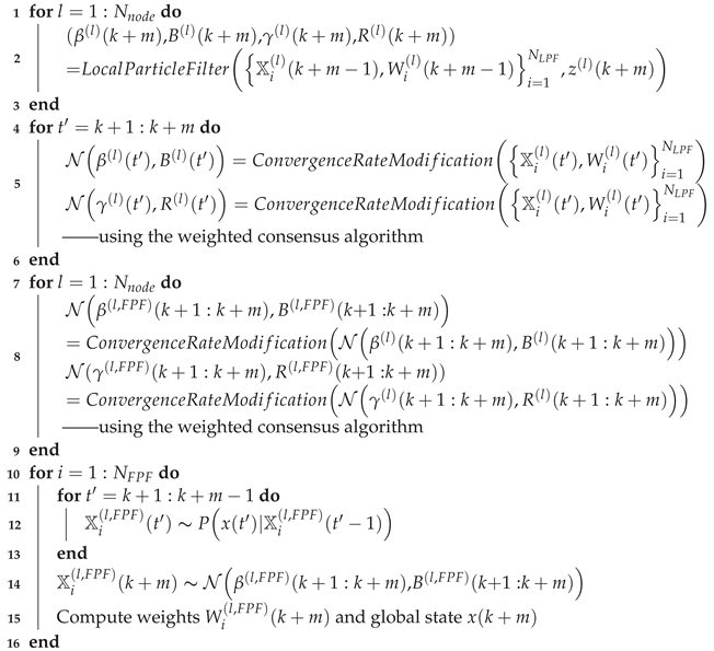
However, if the distribution of sensor nodes is sparse and the communication connection between sensor nodes is dynamic, the tracking result of CF/DPF will show a slow convergence rate and low tracking accuracy. The following figures show the tracking results only with CF/DPF. The simulation environment of Figure 1a is a non-dynamic UWSN, and the communication radius of nodes is longer than that of Figure 1b. The communication network is called the dense network. The simulation environment in Figure 1b is a sparse and dynamic UWSN. It can be seen that the network connection condition changes from a dense network to a sparse and dynamic UWSN, the tracking trajectory fluctuates greatly and the convergence rate is slow. If the CF/DPF can be improved to make it suitable for sparse and dynamic networks, its application fields will be broadened.

3. TASD

In this section, a tracking algorithm for sparse and dynamic underwater sensor networks (TASD) is proposed. Based on the mathematical model of a sparse and dynamic network, the traditional CD/DPF is optimized and improved. The algorithm is optimized to eliminate the influence of invalid nodes in a sparse and dynamic network and maximize the second smallest eigenvalue of the average Laplace matrix.

TASD has two kinds of particle filters that run in parallel, and it has a cascade structure of information flow. Furthermore, the dynamic and sparse characteristic of UWSNs are considered; that is, the communication links between observation nodes change dynamically with a certain probability. Finally, the fusion filtering problem in UWSNs with limited communication energy is considered in TASD.

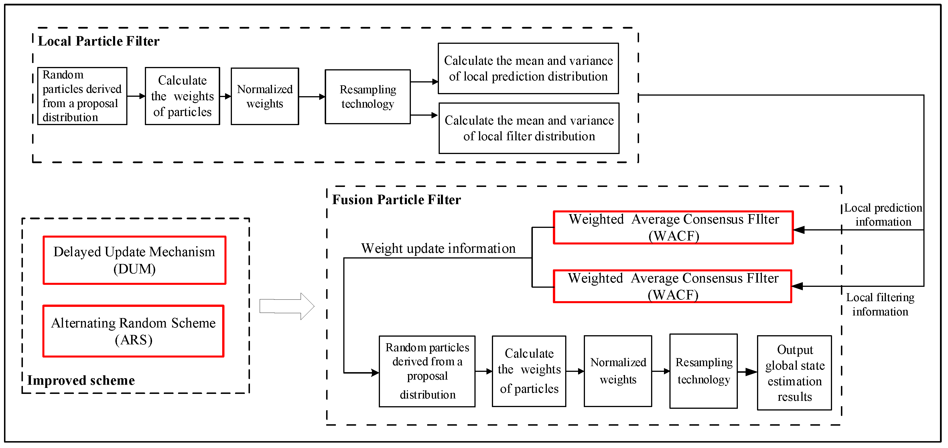
TASD uses the weighted average consensus filter (WACF) to eliminate the influence of invalid nodes, so as to improve the estimation accuracy of CF/DPF. Moreover, TASD adds a delayed update mechanism (DUM) to WACF, which effectively solves the problem of the time difference between the local and fusion particle filters. Not only that, when the energy of sensor nodes is limited, TASD uses an alternating random scheme (ARS) to improve the mean square convergence rate of CF/DPF. The principle of TASD is shown in Figure 2.

3.1. Alternating Random Scheme (ARS)

Based on the assumptions proposed in the paper, in the average network $\overline{G}$, the communication topology of UWSNs with sparse and dynamic characteristics changes randomly and dynamically with a certain probability. In this case, the study of convergence is essential [33]. Therefore, this paper adopts several lemmas, which are all about the convergence of the average consensus algorithm [34]:

Lemma 1.

For an initial state vector $x_0\in {\mathbb{R}}^{N_{node}\times 1}$. At time $t+1$, the state is $x_{t+1}$. $x_{avg}$ is the average consistence value of the state. Moreover, $\rho \left(·\right)$ is the spectral radius. The value of $U_t$ is assumed to be independent and identically distributed,;the convergence of the average consensus algorithm requires a necessary and sufficient condition, which is expressed in a special form as:

$${∥x_{t+1}-x_{avg}∥}_2\le \left({\prod }_{k=0}^t\rho \left(U_t-{11}^T/N_{node}\right)\right){∥x_0-x_{avg}∥}_2$$

(7)

Lemma 2.

If $E\left[\rho \left(U-11^T/N\right)\right]<1$, then $\underset{t\to \infty }{lim}\mathrm{E}{∥x_t-x_{avg}∥}_2=0$.

On the basis of Lemma 2, the mean square convergence factor $C\left(\alpha ,\overline{L}\right)$ and mean square convergence rate $S_g\left(\alpha ,\overline{L}\right)$ of the average consensus algorithm are expressed as:

$$\left\{\begin{array}{c}C\left(\alpha ,\overline{L}\right)=E\left[\rho \left(U-{11}^T/N_{node}\right)\right]\hfill \\ S_g\left(\alpha ,\overline{L}\right)=-lnC\left(\alpha ,\overline{L}\right)=ln{\left(E\left[\rho \left(U-{11}^T/N_{node}\right)\right]\right)}^{-1}\hfill \end{array}\right.$$

(8)

The smaller the value of the mean square convergence factor, the bigger the value of the mean square convergence rate. $\alpha$ is assumed to be assigned the value of $\alpha =1/2d_{max}$, where $d_{max}$ is the maximum communication distance between nodes, and placed in all communication connection edges:

$$C\left(\alpha ,\overline{L}\right) =1-\left(1/2d_{max}\right)E\left[{\lambda }_2\left(L\right)\right] <1,S_g\left(\alpha ,\overline{L}\right) =-ln\left\{1-\left(1/2d_{max}\right)E\left[{\lambda }_2\left(L\right)\right]\right\}$$

(9)

Equation (9) shows the bigger the value of $E\left[{\lambda }_2\left(L\right)\right]$, so as to improve mean square convergence rate. There exists a positive correlation between the values of $E\left[{\lambda }_2\left(L\right)\right]$ and ${\lambda }_2\left(\overline{L}\right)$. It is simple to analyze and calculate the value of ${\lambda }_2\left(\overline{L}\right)$. The larger the value of ${\lambda }_2\left(\overline{L}\right)$, the faster the mean square convergence rate.

Lemma 3.

$\overline{L}$ is the mean Laplace matrix. It is a positive semi-definite matrix, and its eigenvalues can be arranged:

$$0={\lambda }_1\left(\overline{L}\right) \le {\lambda }_2\left(\overline{L}\right) \le {\lambda }_3\left(\overline{L}\right) \le ···\le {\lambda }_N\left(\overline{L}\right)$$

(10)

where ${\lambda }_2\left(\overline{L}\right)>0$ is a necessary and sufficient condition for $\overline{G}$ being connected. In this paper, ${\lambda }_2\left(\overline{L}\right)$ is the algebraic connectivity of the average network communication topology undirected graph $\overline{G}$. The value of ${\lambda }_2\left(\overline{L}\right)$ is directly proportional to the degree of sparse communication topology in UWSNs [35].

TASD is applied to sparse and dynamic UWSNs, the communication connections are assumed to change with probability matrix P dynamically. If the value of ${\lambda }_2\left(\overline{L}\right)$ is blindly increased, not only will the mean square convergence rate improve, the communication energy will increase. However, in practical applications, the energy of communication nodes is limited. In order to maximize the value of ${\lambda }_2\left(\overline{L}\right)$ under the above conditions, an alternating random scheme (ARS) under communication cost constraints is designed to calculate:

$$\underset{\overline{L}}{max}{\lambda }_2\left(\overline{L}\right),s.t.\left\{\begin{array}{c}\overline{L}={\overline{L}}^{\mathrm{T}}\in {\mathbb{R}}^{N\times N},\\ -1\le {\overline{L}}_{ij}\le 0,i,j\in V,i\ne j,\\ \overline{L}1=0,\\ -1/2tr\left(C\overline{L}\right) \le En.\end{array}\right.$$

(11)

The above is a formulaic description of the optimal conditions. $En$ is the maximum value of the energy. C represents a matrix of energy, and it satisfies $C={\left[C_{ij}\right]}_{N_{node}\times N_{node}}^T=C^T$. $C_{ij}$ is the communication energy consumption between nodes i and j, $(1\le i\le N_{node},$$1\le j\le N_{node})$, which is defined as:

$$C_{ij}=\left\{\begin{array}{c}\eta d_{ij}^2,\left(i,j\right)\in \epsilon \\ \infty ,otherwise\end{array}\right.$$

(12)

where $\eta$ is the scale parameter, and $d_{ij}$ represents the Euclidean distance between nodes i and j.

The application of equation mentioned above belongs to the semi-definite programming methods (SDP). The specific method is that SDP is used to adjust the probability matrix P in Assumption 1, dynamically and optimally, then the other matrices related to it will be dynamically optimized. The dynamic calculation process includes the use of (5) and (6). Finally, ${\lambda }_2\left(\overline{L}\right)$ is maximized to achieve the overall dynamic topology optimization function.

To summarize, ARS optimizes the mean square convergence rate of the fusion particle filter. The improvement of the mean square convergence rate shortens the time delay of fusion filtering, which can be described as “killing two birds with one stone”. It is worth mentioning that the design of ARS is based on the condition that the energy of sensor nodes is limited, which makes the service conditions of TASD meet the reality.

3.2. Weighted Average Consensus Filter (WACF) with Delayed Update Mechanism (DUM)

Lemma 4.

If ${\lambda }_2\left(\overline{L}\right) >0$, then $\overline{G}$ is connected. The average consensus algorithm is given by:

$$x_{k+1}^n=W_k^{nn}{x}_k^n+{\sum }_{l\in N_k^n}{W}_k^{nl}{x}_k^l,\forall n,l\in V$$

(13)

The state estimation variables $x_k$ of all observation nodes will converge to the average consensus value $x_{avg}$; that is $\underset{k\to \infty }{lim}E{∥x_k-x_{avg}∥}_2=0$. Moreover, $x_k^n$ is the state variable of node $n\left(n\le N_{node}\right)$ at k. $N_k^n= \left\{l\in V|\left(n,l\right)\in {\epsilon }_k\right\}$ represents the set of neighboring nodes for node $n\left(n\le N_{node}\right)$. $W_k^{nl}$ and $W_k^{nn}$ are weights and satisfy $W_k^{nn}+{\sum }_{l\in N_k^n}{W}_k^{nl}=1$. At the same time, if the initial state vector is $x_0$, then the average consensus value is $x_{avg}={11}^{\mathrm{T}}/N_{node}{x}_0$, where 1 is the unit column vector [33].

TASD uses WACF of (13) in Lemma 4 to estimate the local particle filter distribution and local particle prediction distribution with Gaussian approximation. However, the application environment of this paper is sparse and dynamic UWSN, and the weight matrix is “time-varying” and each element in the weight matrix is given by ARS in Section 3.1.

The form of vector representation of the algorithm shown in (13) is:

$${\psi }_{k+1}={\prod }_{t=0}^k{W}_t,x_{k+1}={\psi }_{k+1}{x}_0$$

(14)

Based on the average network model of sparse and dynamic UWSN, the weight matrix is $W_k=I-\alpha {\overline{L}}_k$. Then, the average weight matrix corresponding to the average network model is $\overline{W}=I-\alpha \overline{L}$. The convergence characteristics of (14) are analyzed, based on Lemma 4. Then (14) converges to the average consensus value $x_{avg}={11}^{\mathrm{T}}/N_{node}{x}_0$. Moreover,

$$x_{avg}=\underset{k\to \infty }{lim}{x}_k=\underset{k\to \infty }{lim}\left({\prod }_{t=0}^{k-1}{W}_t\right)x_0=\underset{k\to \infty }{lim}{\psi }_k{x}_0={11}^{\mathrm{T}}/N_{node}{x}_0$$

(15)

It is assumed that the fusion particle filter has run to the iteration $k\left(1\le k\right)$. Moreover, the local particle filter and the fusion particle filter are not synchronized. There are m iterative steps between them. Therefore, WACF (13) is used to reach consensus by outputs of local particle filter. If $\overline{G}$ is connected, then the outputs of the four weighted consensus filters will converge asymptotically to the weighted average consensus values. With the addition of a delayed update mechanism (DUM), WACF eliminates the asynchronous interference of the two filters.

The information of communication topology changes with time, such as the connection matrix, Laplace matrix, degree matrix, and weight matrix. The classical average consensus method is selected in CF/DPF. Compared with the classical method, WACF with time-varying weight matrix is more reasonable. The dynamic weight matrix effectively suppresses the influence of invalid nodes on the filtering results and improves the filtering accuracy. With the aid of DUM, the asynchronous problem caused by two filters in a series is also solved.

3.3. Algorithm Analysis

(1)

Analysis of TASD implementation steps.

The analysis of the TASD will described in this part and the pseudo code is in Algorithm 1. Firstly, the basic application background of the algorithm is briefly introduced.

The sparse and dynamic UWSN is composed of $N_{node}$ nodes. The state vector $x={\left[x_1,x_2,...,x_{n_x}\right]}^T$ is $n_x$-dimensional. In most cases, $n_x=4$ and $x={\left[x_1,x_2,x_3,x_4\right]}^T$. The four-dimensional variables here represent the horizontal position coordinates, the longitudinal position coordinates, the transverse velocity, and the longitudinal velocity, respectively. At time k, node $l(1\le l\le N_{node})$ has a measurement $z^{\left(l\right)}\left(k\right)$. Then, $z={\left[z^{\left(1\right)T},z^{\left(2\right)T},...,z^{\left(N_{node}\right)T}\right]}^T$ is the global observation vector. $N_{LPF}$ and $N_{FPF}$ represent the number of particles for the local particle filter and fusion particle filter, respectively. Moreover, the operation steps of the fusion particle filter are m steps slower than that of the local particle filter. Finally, node n at time k has the mean ${\beta }^{\left(n\right)}\left(k\right)$ and variance $B^{\left(n\right)}\left(k\right)$ of local filtering distribution. Similarly, it also has the mean ${\gamma }^{\left(n\right)}\left(k\right)$ and variance $R^{\left(n\right)}\left(k\right)$ of the local prediction distribution.

(2)

Computational complexity.

When improving the traditional scheme, if the complexity of the algorithm is blindly increased in order to pursue high location accuracy, it is not worth the loss. Therefore, the computational complexity of CF/DPF and TASD is simply compared in this paper. In the application field of target tracking, the internal computing equipment of observation nodes is generally implemented in the form of discrete recursion. Then the filtering calculation time becomes a crucial problem, which could be used to evaluate the efficiency of filtering algorithm. However, there are many factors that affect the actual calculation time of filtering, such as the performance of software used in the experimental operation, the configuration of the hardware equipment, communication factors, and programming methods. Therefore, it is difficult to have a uniform conclusion through strict theoretical proof. In this paper, floating point operations (Flops) in [36] are used to evaluate complexity computation. It contains floating-point multiplication, division, addition, and subtraction, but does not include logical operations.

Firstly, the computational complexity of CF/DPF is analyzed. The CF/DPF runs two complete particle filters, local particle filter, and fusion particle filter. Node $l(1\le l\le N_{node})$ has the computational complexity of the local particle filter as $\mathrm{O}\left(N_{node}{n}_x^2{N}_{LPF}\right)$; the computational complexity of the fusion filter is $\mathrm{O}\left(N_{node}{n}_x^2{N}_{LPF}\right)$. The average consensus filter is inserted into the series structures of the two filters. Corollary 5.2 and Theorem 8.4 in [37] are cited, which are called Lemmas 5 and 6 in this paper.

Lemma 5.

Concerning the convergence time for the equal-neighbor, time-invariant, symmetric model on a connected graph on $N_{node}$ nodes, its convergence time is defined as:

$$T_{N_{node}}\left(\alpha \right) =\mathrm{O}\left(N_{node}^{3}log\left(N_{node}/\alpha \right)\right)$$

(16)

Furthermore, for every positive integer $N_{node}$, there exists an $N_{node}$-node connected graph for which $T_{N_{node}}\left(\alpha \right) =\mathsf{\Omega }\left(N_{node}^{3}log\left(1/\alpha \right)\right)$. According to the definition of $\mathrm{O}$ and $\mathsf{\Omega }$ in [32], the CF/DPF’s computational complexity is obtained:

$$max\left\{N_{node}{n}_x^2\left(N_{LPF}+N_{FPF}\right),n_x^2{N}_{node}^{3}log\left(1/\alpha \right)\right\}$$

(17)

Lemma 6.

There exists a connected graph on $N_{node}$ nodes and a constant $\kappa >0$. The convergence time is defined as:

$$T_{N_{node}}\left(H,\alpha \right) \le \kappa H{N}_{node}^{3}log\left(1/\alpha \right)$$

(18)

For connection topology $G_k= \left(V,{\epsilon }_k\right)$, $\left|V\right| =N_{node}$, there exists iterative time series H and k; that $G_k= \left(V,{\epsilon }_{k\mathrm{H}}\cup {\epsilon }_{k\mathrm{H}+1}\cup ···\cup {\epsilon }_{\left(k+1\right)\mathrm{H}-1}\right)$ is strongly connected. Moreover, (18) assumes that the topology is dynamic, so it is upper bound. The computational complexity of the TASD is:

$$max\left\{N_{node}{n}_x^2\left(N_{LPF}+N_{FPF}\right),n_x^{2}H{N}_{node}^{3}log\left(1/\alpha \right)\right\}$$

(19)

From (17) and (19), it can be seen that the highest power of the expression of computational complexity is nearly the same, and the amount of computation does not change greatly.    

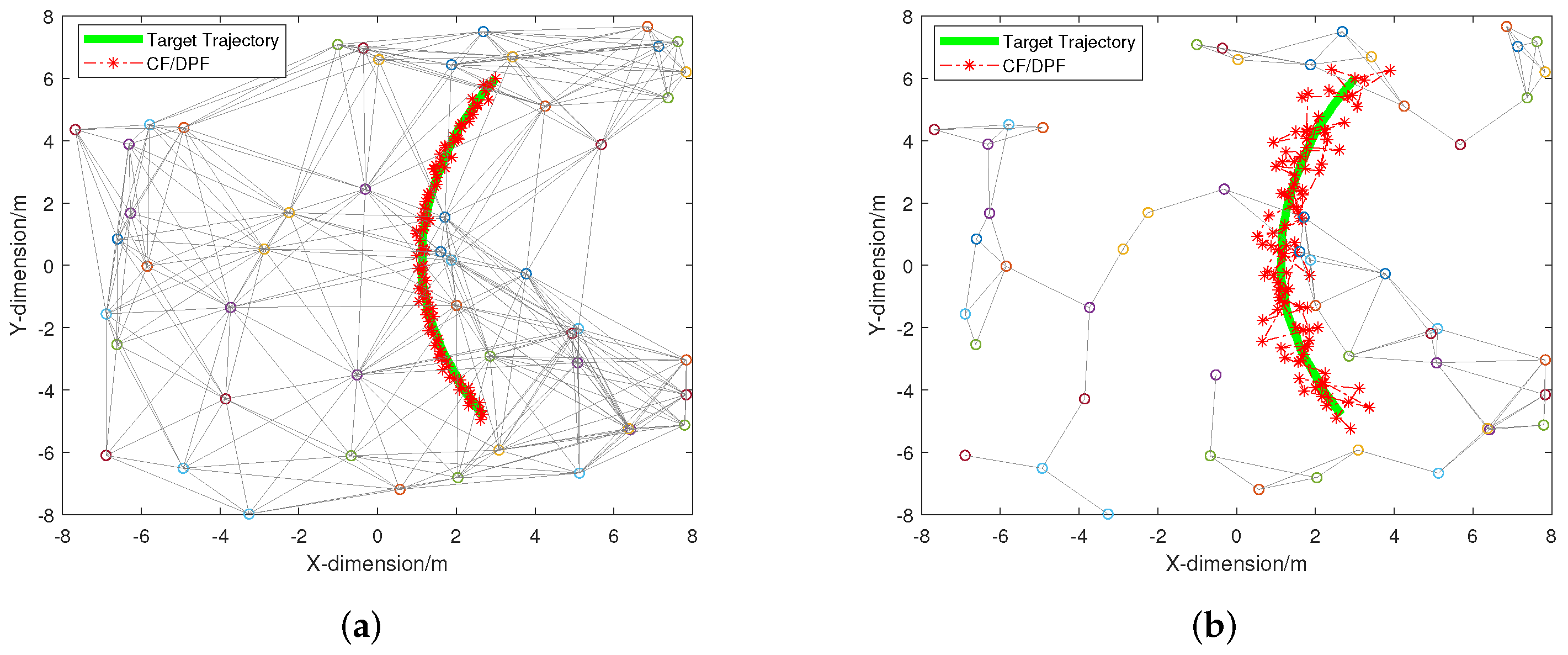
Algorithm 1: A tracking algorithm for sparse and dynamic underwater sensor networks

Input: ${\left\{{\mathbb{X}}_i^{\left(l\right)}(k+m-1),W_i^{\left(l\right)}(k+m-1)\right\}}_{i=1}^{N_{LPF}}$ particle set and weight set of the local particle filter.  Output: Estimation of global state $x\left(k+m\right)$.

4. Simulation and Analysis

In order to facilitate the labeling expression for the subsequent simulation experiments, CF/DPF and TASD are used to represent the traditional multi-rate consensus/fusion filtering algorithm and the tracking algorithm for sparse and dynamic UWSNs, respectively. Before the simulation verification, it is necessary to illustrate and specify the main indices of performance. Firstly, several types of images are obtained by the simulation software, including comparisons of tracking trajectories, comparisons of errors, and comparisons of convergence rates. In order to verify the universality of TASD in practical application, two groups of simulation experimental environments are set up in this paper: Example 1 and Example 2, respectively. Compared with Example 1, Example 2 has more nodes, a larger monitoring range, sparser node distribution, and stronger dynamic characteristics of communication topology.

The average estimated error (AE) used to measure the accuracy of distributed estimation is defined:

$$A{E}_k=\sqrt{\left(1/N_{node}\right){\sum }_{i=1}^{N_{node}}∥{\widehat{x}}_k^i-{x_k∥}_2}$$

(20)

The weighted average consensus tracking error (WE) is used to measure the convergence rate of the algorithm:

$$W{E}_k=\sqrt{\left(1/N_{node}\right){\sum }_{i=1}^{N_{node}}∥{\widehat{x}}_k^i-{x_{k,avg}∥}_2}$$

(21)

${\widehat{x}}_k^i$ is the estimation of the state variable for node $i\left(1\le i\le N_{node}\right)$ at time k. $x_k$ is the real state variable of the target. Moreover, $x_{k,avg}$ is the weighted consensus state variable of the target.

How are the sparse and dynamic characteristics of the simulations reflected? Firstly, all communication links are not necessarily connected at each iteration step, and they change randomly with probability P. This reflects the dynamic characteristics. Secondly, if the communication radius R is small, then the number of neighbors of each node is small, too. The condition cannot satisfy the maximum number of communication connection sides. Moreover, some nodes have no neighboring nodes or some invalid nodes (no observation information) as a result of the limitation of sensing radius $R1$. This reflects the characteristics of sparse.

Example 1.

Small-scale sparse and dynamic UWSN.

The simulation scenario in Example 1 adopts the bearing-only tracking (BOT) model in [38], which is a non-linear model. Observations and prior knowledge are used to estimate state variable of four dimensions. The state variable at time k is $x\left(k\right) = \left[X\left(k\right),Y\left(k\right),\dot{X}\left(k\right),\dot{Y}\left(k\right)\right]$. The system state model is described in (2). In this section, $x_k$ is replaced by $x\left(k\right)$ and $x_{k-1}$ is replaced by $x\left(k-1\right)$. Then, the state function is given by:

$$f\left(x\left(k\right),k+1\right) =\left[\begin{array}{cccc}1& 0& \frac{sin\left(\mathsf{\Phi }\left(k\right)\mathsf{\Delta }T\right)}{\mathsf{\Phi }\left(k\right)}& -\frac{1-cos\left(\mathsf{\Phi }\left(k\right)\mathsf{\Delta }T\right)}{\mathsf{\Phi }\left(k\right)}\\ 0& 1& \frac{1-cos\left(\mathsf{\Phi }\left(k\right)\mathsf{\Delta }T\right)}{\mathsf{\Phi }\left(k\right)}& \frac{sin\left(\mathsf{\Phi }\left(k\right)\mathsf{\Delta }T\right)}{\mathsf{\Phi }\left(k\right)}\\ 0& 0& cos\left(\mathsf{\Phi }\left(k\right)\mathsf{\Delta }T\right)& -sin\left(\mathsf{\Phi }\left(k\right)\mathsf{\Delta }T\right)\\ 0& 0& sin\left(\mathsf{\Phi }\left(k\right)\mathsf{\Delta }T\right)& cos\left(\mathsf{\Phi }\left(k\right)\mathsf{\Delta }T\right)\end{array}\right]$$

(22)

With $\mathsf{\Phi }\left(k\right) =A_m/\sqrt{{\dot{X}}^2\left(k+1\right)+{\dot{Y}}^2\left(k+1\right)}$. $A_m$ is called the acceleration parameter and set to $1.08\times 10^{-5}\mathrm{units}/{\mathrm{s}}^2$ by [38].

The function of the observation is:

$$h^n\left(x\left(k\right),k\right) = \mathrm{atan}\left(\left(X\left(k\right)-X^{\left(n\right)}\right)/\left(Y\left(k\right)-Y^{\left(n\right)}\right)\right)$$

(23)

The flicker noise in [39] is used as the observation noise. The likelihood model is described as:

$$P\left(z^{\left(n\right)}|x\left(k\right)\right) =\vartheta \times \mathcal{N}\left(x;0,{10}^4{\sigma }_{{\nu }^{\left(n\right)}}^2\left(k\right)\right) + \left(1-\vartheta \right) \times \mathcal{N}\left(x;0,{\sigma }_{{\nu }^{\left(n\right)}}^2\left(k\right)\right)$$

(24)

where $\vartheta =0.09$. The value of the noise variance ${\sigma }_{{\nu }^{\left(n\right)}}^2$ depends on the distance $r^{\left(n\right)}\left(k\right)$ between the node $n\left(1\le n\le N_{node}\right)$ and the target [40]:

$${\sigma }_{{\nu }^{\left(n\right)}}^2\left(k\right) =0.08r^{{\left(n\right)}^2}\left(k\right) +0.1150r^{\left(n\right)}\left(k\right) +0.7405$$

(25)

$N_{node}=50$ sensor nodes are distributed in UWSN. The communication radius of each sensor node is $R=\sqrt{2log\left(N_{node}\right)/N_{node}}$. The observation information can be exchanged among the nodes within the communication range for the compensation and adjustment of their own data. Moreover, each sensor node has a sensing radius $R1=R$, the node can observe and estimate the target’s position only with the target in the observation range. The position of the tracking target is initialized. It starts from position (3, 6), and the first three iterations are (2.9226, 5.8991), (2.8503, 5.7962), and (2.7673, 5.6855). The number of particles in the local particle filter is the same as that of the fusion particle filter, $N_{LPF}=N_{FPF}=500$.

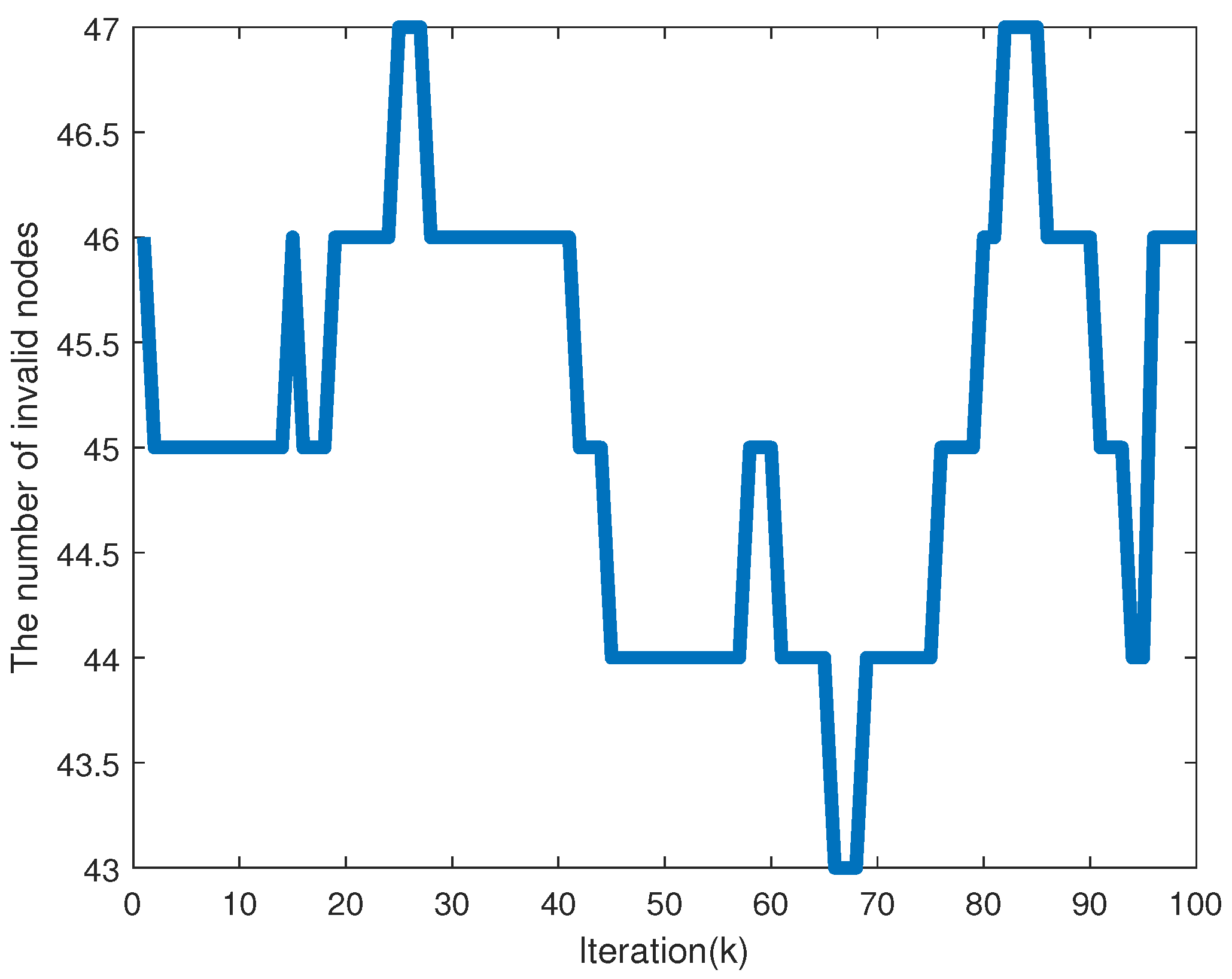
The invalid nodes in each filtering step are counted. The statistical results are shown in Figure 3. It can be seen that the number of invalid nodes remains high. The least number of invalid nodes occurs between 60 to 70 iterations, However, the least number of invalid nodes accounts for a large proportion of total nodes. The observation results of these invalid nodes will lead to consensus errors; the accuracy of the final filtering result is low, and a divergent phenomenon occurs. If there is no limit, the maximum number of connected edges is $M_{max}=N_{node}(N_{node}-1)/2=1225$. In the simulations, the number of communication connection sides cannot reach the ideal maximum due to the limitation of communication distance and communication energy. The probability of an effective communication connection between any node n and $\left(1\le n\le N_{node},1\le l\le N_{node},n\ne l\right)$ in the communication range obeys the Bernoulli distribution, in that the neighboring nodes may be disconnected.

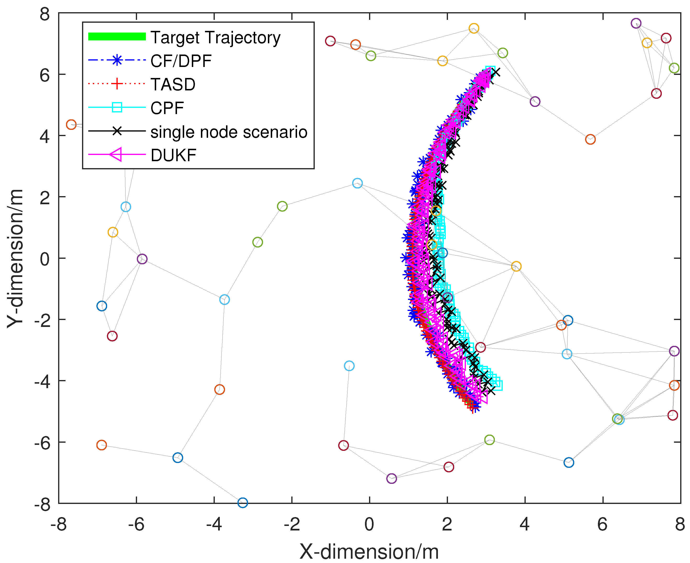
Figure 4 shows the target’s trajectory, CF/DPF and TASD’s tracking trajectory, as well as the tracking trajectory of an arbitrary observation node randomly selected. Each hollow circle represents an observation node, if there is a line between the two nodes, it means that the two observation nodes can communicate with each other. The maximum energy consumption $En$ can be calculated. The number of connecting edges is 56, $M_k\ll M_{max}$. Therefore, if the undirected graph is connected, the UWSN formed in Figure 4 is a sparse and dynamic UWSN. The tracking trajectory of the CF/DPF fluctuates greatly around the true trajectory of the target and has a large deviation and divergence. This is because sparse and dynamic topology communication conditions affect CF/DPF. However, the trajectory of the TASD is smooth and has little fluctuation. The trajectory curve observed by a single node obviously deviates from the motion trajectory of the target, because the node may not be able to observe the target at every time. The observation trajectory divergence of the centralized particle filter algorithm (CPF) is obvious, which may be caused by the failure of the fusion center and failure of the dynamic adjustment of weight. The distributed unscented Kalman filter algorithm (DUKF) is similar to the CF/DPF algorithm. Their trajectories are roughly the same as those of the target, but the jitter is obvious. The tracking trajectory of TASD almost coincides with the real trajectory of the target. This is because TASD is suitable for sparse and dynamic UWSN. It can continuously and efficiently track the target. In contrast, TASD has the best tracking trajectory in sparse and dynamic UWSN.

In order to analyze the tracking accuracy of CF/DPF and TASD intuitively, the average estimation errors of the two algorithms will be compared. Figure 5 shows a comparison of the average estimation errors between CF/DPF and TASD. Abscissa is the iteration steps of the simulation, and ordinate is the error value. The average estimation errors of CF/DPF are between 0.05 to 1.35 m, and the amplitude of the curve is larger than that of the TASD. The curve does not show a uniform convergence trend, but tends to diverge. Because the traditional consensus scheme used by CF/DPF has no weight matrix adjustment, it does not take into account the different confidence of each node. The nodes with unreliable information are assigned the same weight as other nodes, so the cumulative estimation error is large. However, the average estimation error curve of TASD is gentler than that of CF/DPF. The fluctuation range of the curve is from 0 to 0.1 m and it tends to converge. The average estimation error of TASD is 92.6% lower than that of CF/DPF. This excellent error result is due to the WACF with DUM. WACF assigns different weights to different particles and nodes, and the weight matrix also changes with the change of dynamic topology. In this way, the content of reliable information accounts for a larger proportion, and the part of unreliable information is reduced or even ignored. Therefore, the final estimation result is more accurate. It is not difficult to see that our TASD has higher estimation accuracy than CF/DPF.

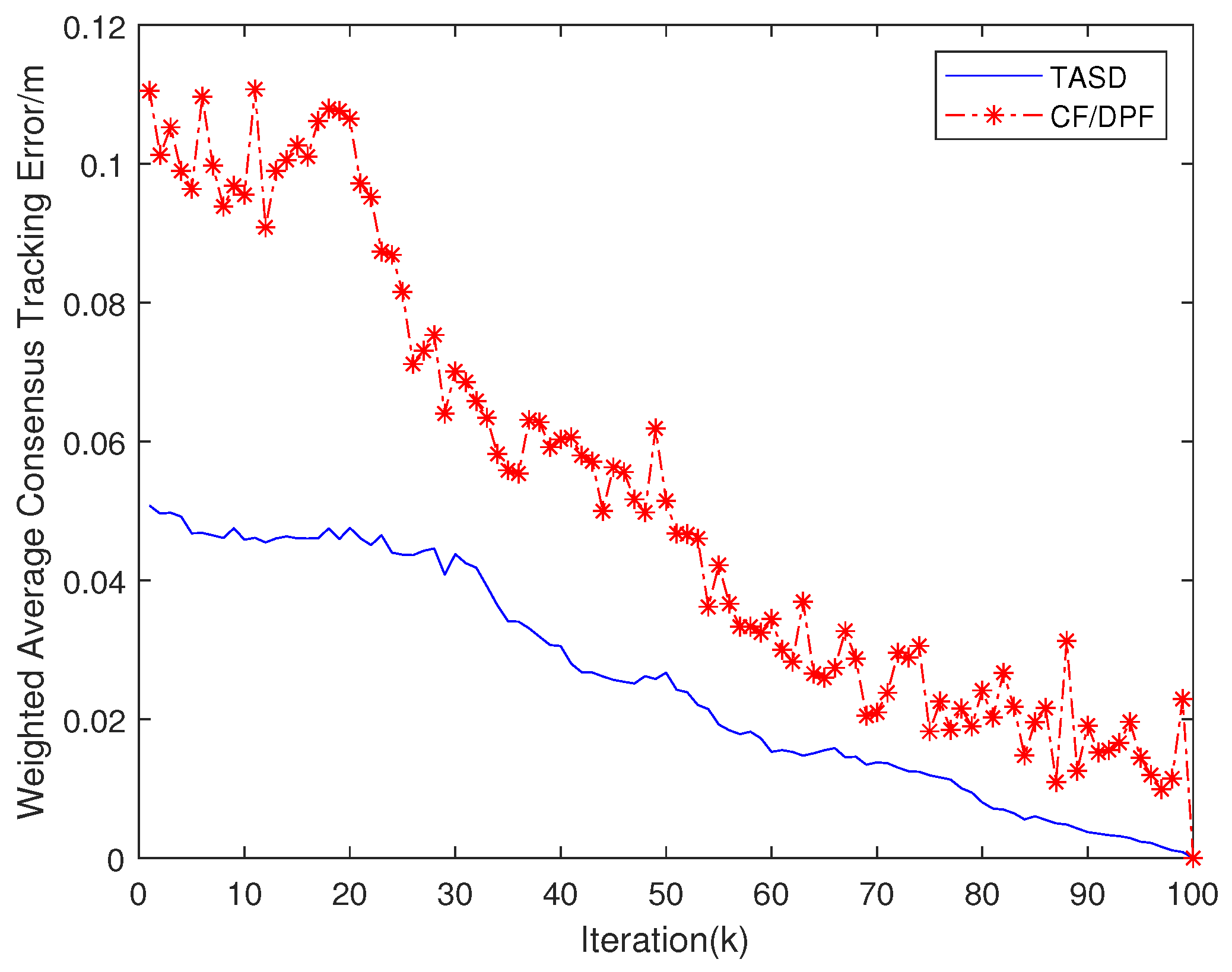
Figure 6 shows the weighted average consensus tracking error of CF/DPF and TASD. This comparison graph is used to reflect the convergence rate of the consensus algorithm. The fluctuation of the connecting points of the CF/DPF’s curve is obvious, and it also shows a large jump in the final convergence process. The curve of TASD is smoother than CF/DPF’s curve, and it converges faster than that of CF/DPF. The weighted consensus tracking error of TASD is reduced by 82.3% compared with CF/DPF. This is because TASD uses ARS to adjust the fusion particle filter. ARS improves the mean square convergence rate of WACF when considering the energy limitation of nodes. It can be seen that TASD has a faster and better mean square convergence rate than CF/DPF.

Example 2.

Large-scale sparse and dynamic UWSN.

According to the simulation environment of [38]. Equation (2) is used as the state model. Four dimensional state variables $x\left(k\right) = \left[X\left(k\right),Y\left(k\right),\dot{X}\left(k\right),\dot{Y}\left(k\right)\right]$. The process noise $Q=k_w^2\times I_4$ and $k_w=4$. The observation model is:

$$z_k^n= \left[\begin{array}{c}{\rho }_k^n\\ {\phi }_k^n\end{array}\right] = \left[\begin{array}{c}\sqrt{{\left(x_k^t-x^n\right)}^2+{\left(y_k^t-y^n\right)}^2}\\ arctan\left(y_k^t-y^n\right)/\left(x_k^t-x^n\right)\end{array}\right] + {\nu }_k^n$$

(26)

where ${\rho }_k^n$ and ${\phi }_k^n$ represent the distance and angle between the tracking target and the node $n\left(1\le n\le N_{node}\right)$ at time k, $\left(1\le k\right)$, respectively. The covariance of observation noise is $R_k^n=E\left[v_k^{n}v{{}_k^n}^T\right] =k_v^2\times I_2$ and $k_v=2$.

The simulation environment is a large-scale sparse and dynamic UWSN. The number of nodes is $N_{node}=100$, and the area is expanded to 100 m × 100 m. The communication distance of these sensor nodes is set to $R=\sqrt{N_{node}}$. The green solid line in Figure 7 is the true trajectory of the tracking target, the sampling time is 1s, and the total number of sampling steps is set to 200 here. The maximum number of communication connection edges between these sensor nodes is $M_{max}=N_{node}\left(N_{node}-1\right)/2=4950$. The number of connected edges in Figure 7 is 268. Moreover, whether the connected edges in the graph are connected must obey the assumptions in the previous paper. Then the background of this simulation experiment meets the requirements of large sparse and dynamic UWSN.

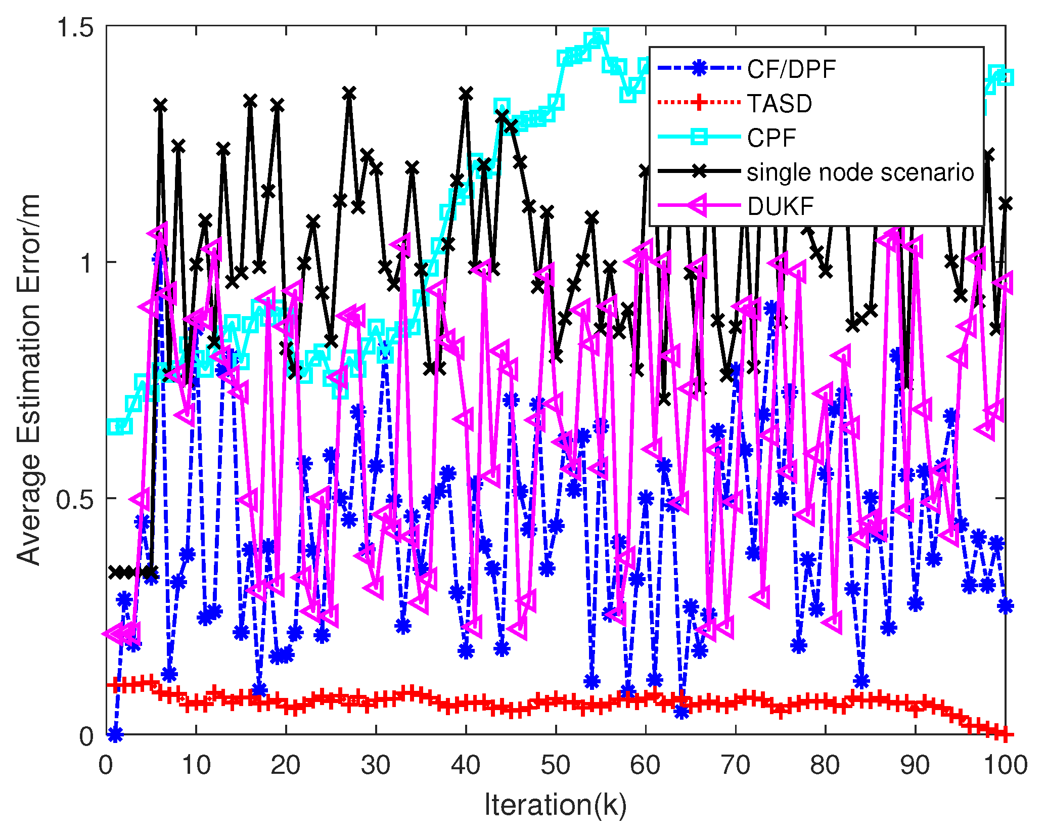
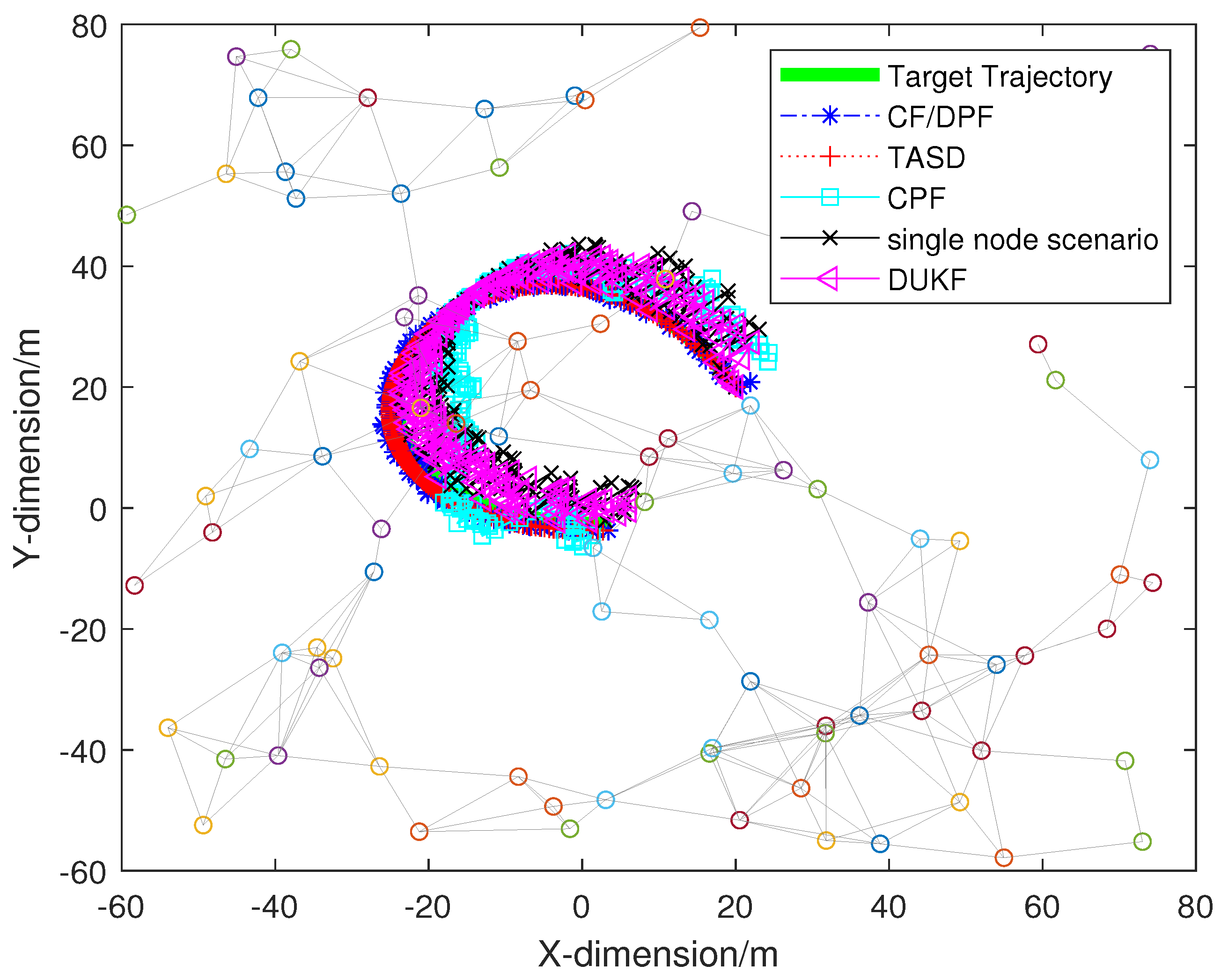
Figure 7 shows the comparison of tracking trajectories. The comparison includes CF/DPF, TASD, and an arbitrary node. The trajectory of CF/DPF jumps greatly and is not stable, the convergence trend is not obvious. Due to the limitation of observation distance, the observation trajectory of a single node deviates from the target trajectory more obviously. The trajectory of a centralized particle filter algorithm has obvious divergence, which is caused by the fusion center and invalid nodes. The tracking trajectory curve of distributed unscented Kalman filter is similar to that of CF/DPF. The tracking trajectory of TASD almost coincides with the true trajectory of the tracking target. The whole tracking trajectory is smooth without obvious jumping, and the convergence trend is obvious. When we merely look at the tracking trajectories, we can see that TASD has a better tracking ability than CF/DPF. The specific error situation needs further analysis to reach a conclusion.

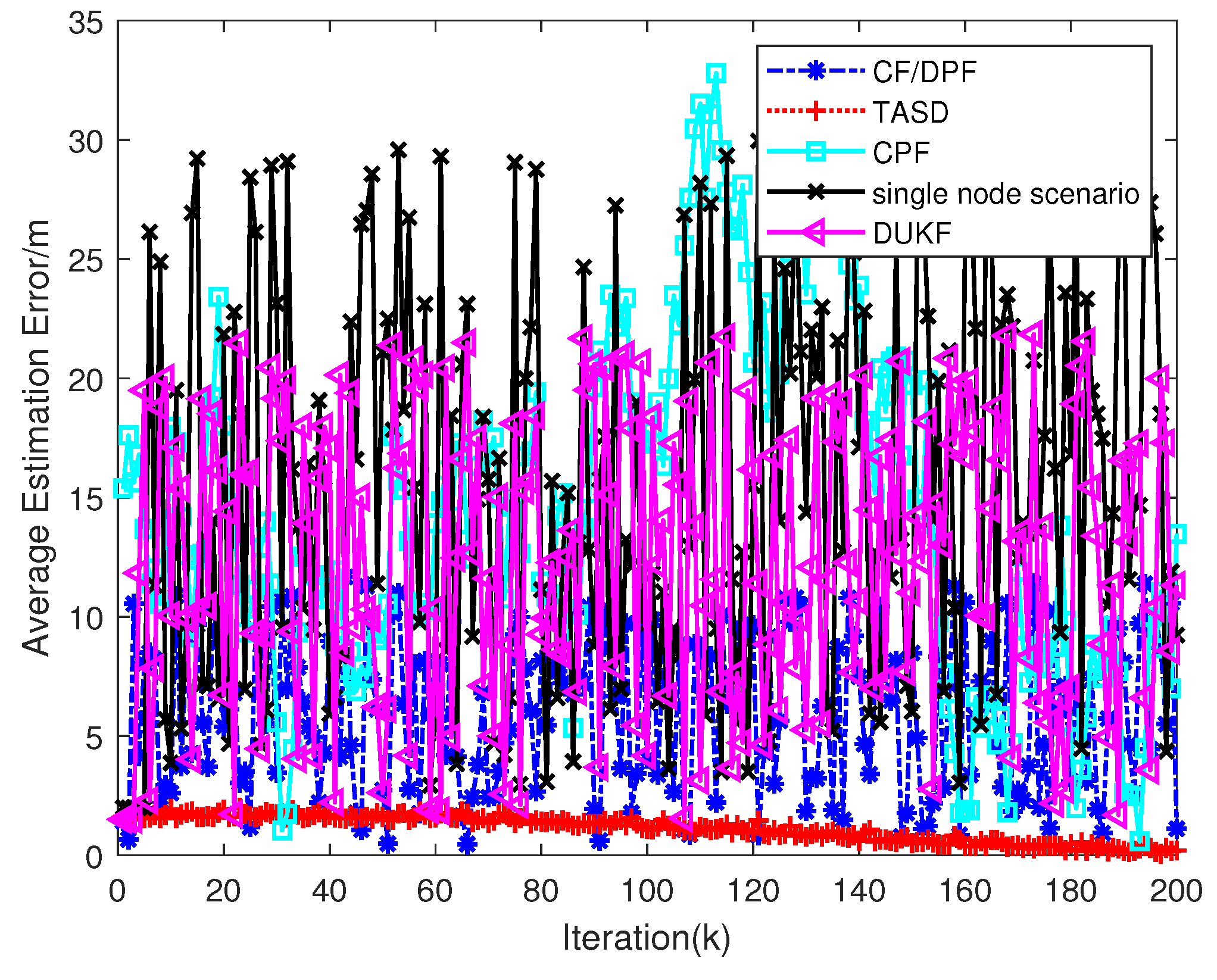
The average estimation error is shown in Figure 8. It can be seen that the average estimation error curve of CF/DPF fluctuates between 0 and 30 m, with a large fluctuation range and has no obvious convergence trend. This is because CF/DPF does not have any regulation scheme and it is not suitable for sparse and dynamic UWSNs. The difference is, the average estimation error curve of TASD fluctuates from 0 to 3 m, the fluctuation amplitude is small, and the curve tends to converge to 0 m. The average estimation error of TASD is 90% lower than that of CF/DPF. This is because WACF regulates the weights of invalid nodes, which retains higher accuracy estimation results in the fusion process. Moreover, DUM compensates for the time difference between the filters. Therefore, the estimation accuracy of TASD is higher than CF/DPF.

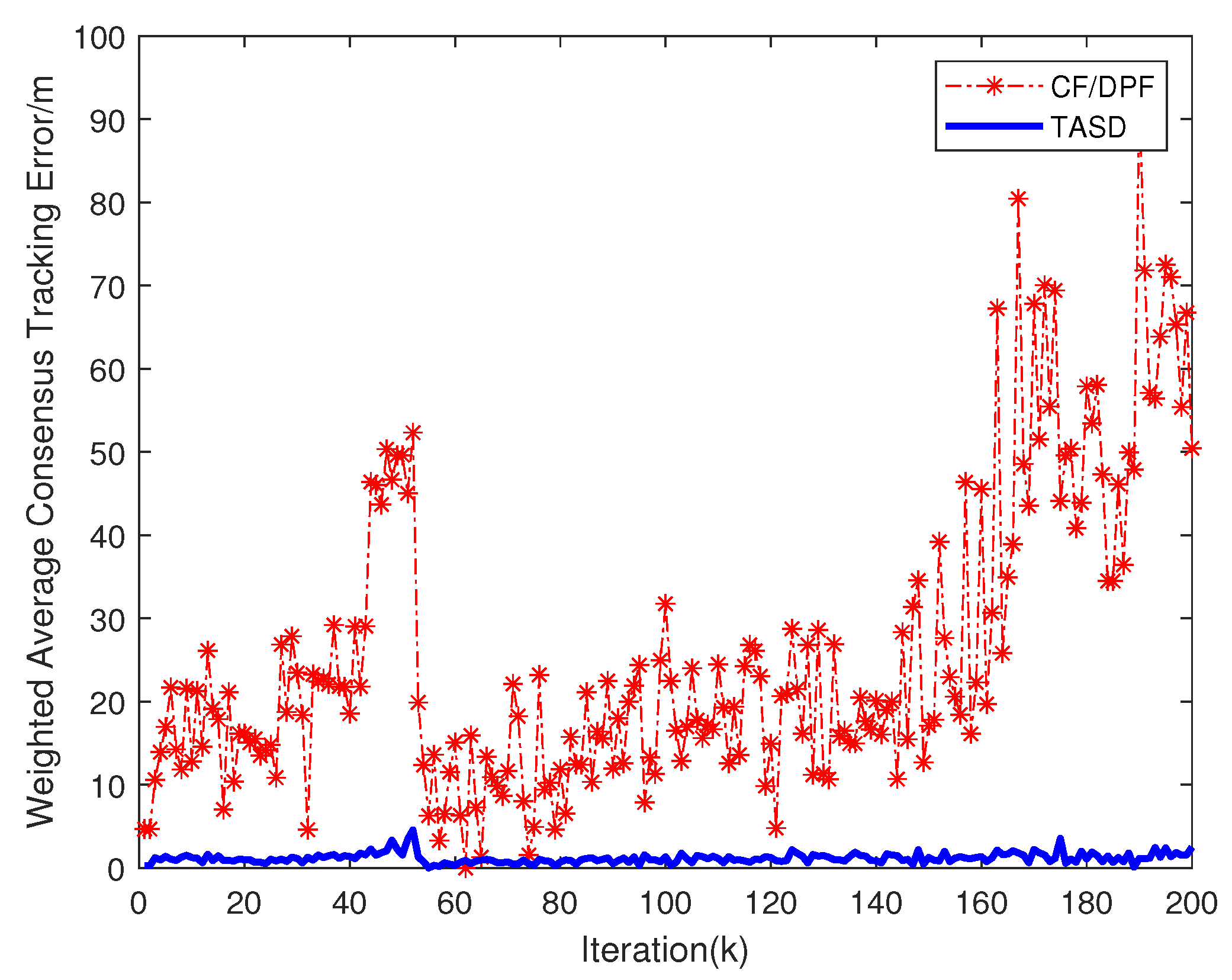
Figure 9 presents the comparisons of weighted average consensus tracking errors. It can be seen that the weighted average consistent tracking error curve of CF/DPF fluctuates in the range of 0 to 90 m, with a large fluctuation range, and it has no convergence trend. The mean square convergence rate of the traditional consensus algorithm has not been optimized and can only converge by virtue of its own advantages. Therefore, the convergence error effect of CF/DPF is not ideal. Whereas the weighted average consensus tracking error curve of TASD fluctuates from 0 to 10 m, with a small fluctuation range, and is gentle. The weighted consensus tracking error of TASD is reduced by 88.9% compared with CF/DPF. This is not only due to the adoption of WACF, but also due to the addition of ARS. ARS maximizes the mean square convergence rate when the node energy is limited.

5. Conclusions

In a sparse and dynamic UWSN, the communication between nodes is unstable. Furthermore, in practical application, the system model is nonlinear and the noise is non-Gaussian. A tracking algorithm for sparse and dynamic UWSNs based on a particle filter is proposed. Two kinds of particle filters are run simultaneously on each sensor node. Firstly, the local particle filter uses the local observation information to estimate the state variable. It also transmits the filtering information to the next fusion filter. Then, in the fusion particle filter, the weighted average consensus filter is used to process the input information. Thus, the difference in reliability of state estimation among all nodes can be reasonably eliminated. Besides, the mean square convergence rate of the fusion filter is optimized under the condition of limited communication energy consumption. Finally, the global filtering results are output. In the future, the output of the fusion filter will be fed back to the local particle filter. Such a closed-loop feedback operation can modify the filtering result of the local particle filter and obtain a more accurate global state estimation result.