
Establishing a Risk Assessment Framework for Marine Assets and Assessing Typhoon Lekima Storm Surge for the Laizhou Bay Coastal Area of the Bohai Sea, China


Abstract
1. Introduction
1.1. Research Status
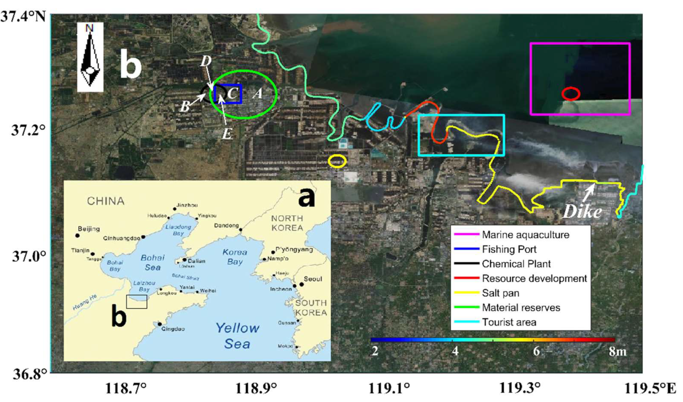
1.2. Study Area
1.3. Typhoon Dynamics
2. Data and Methods
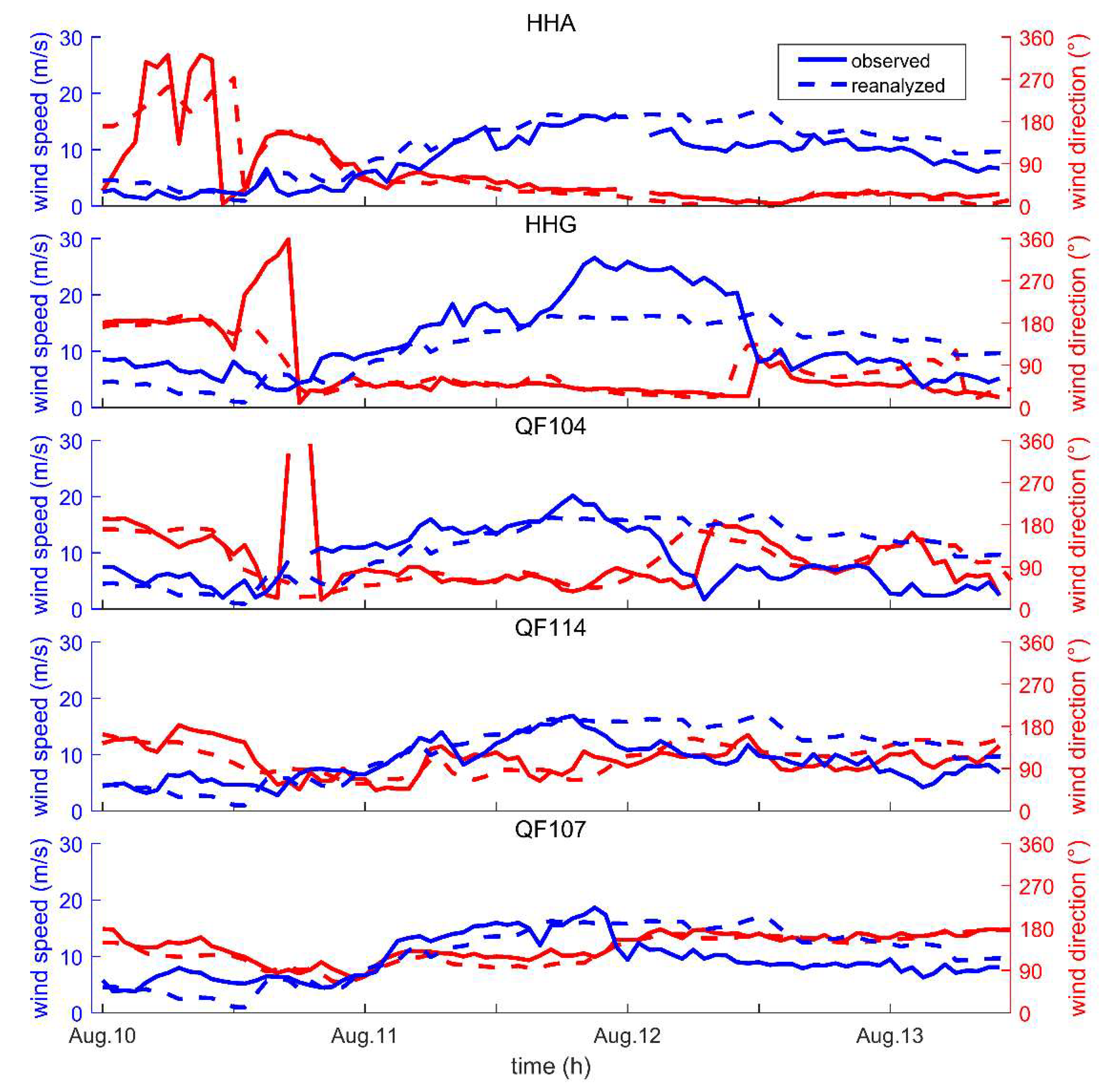
2.1. Observed Data
2.2. Calculation of Return Period
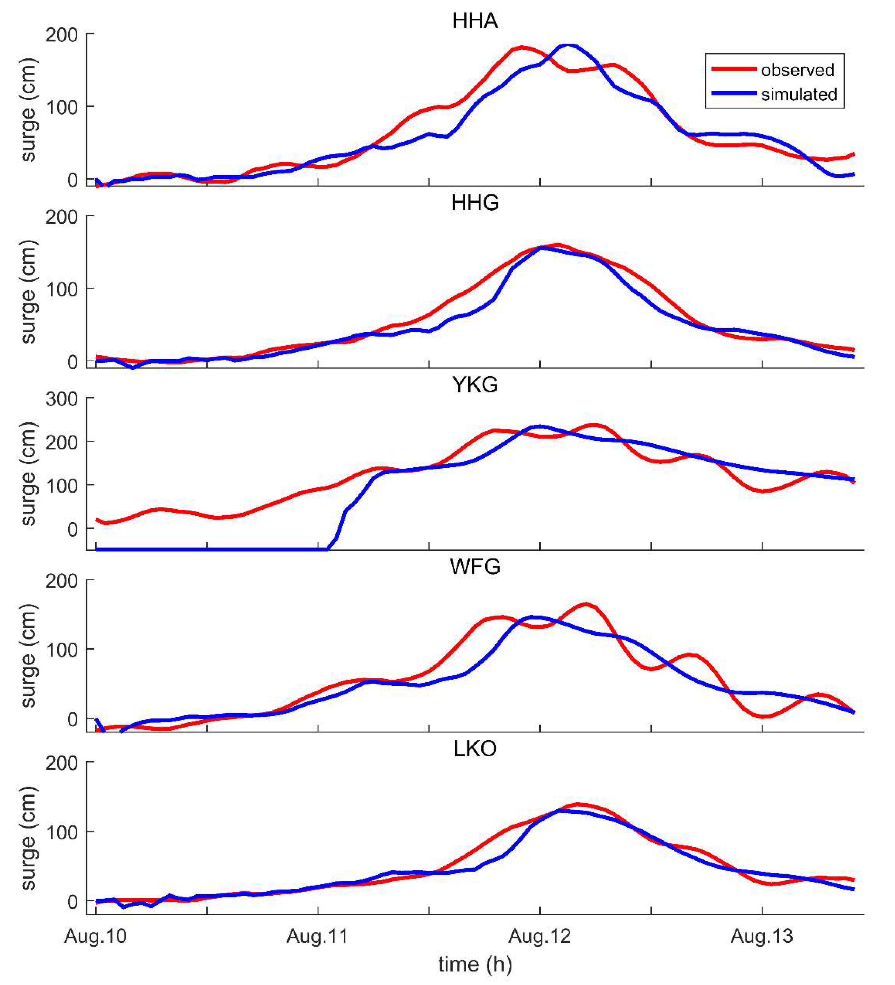
2.3. Model and Validation
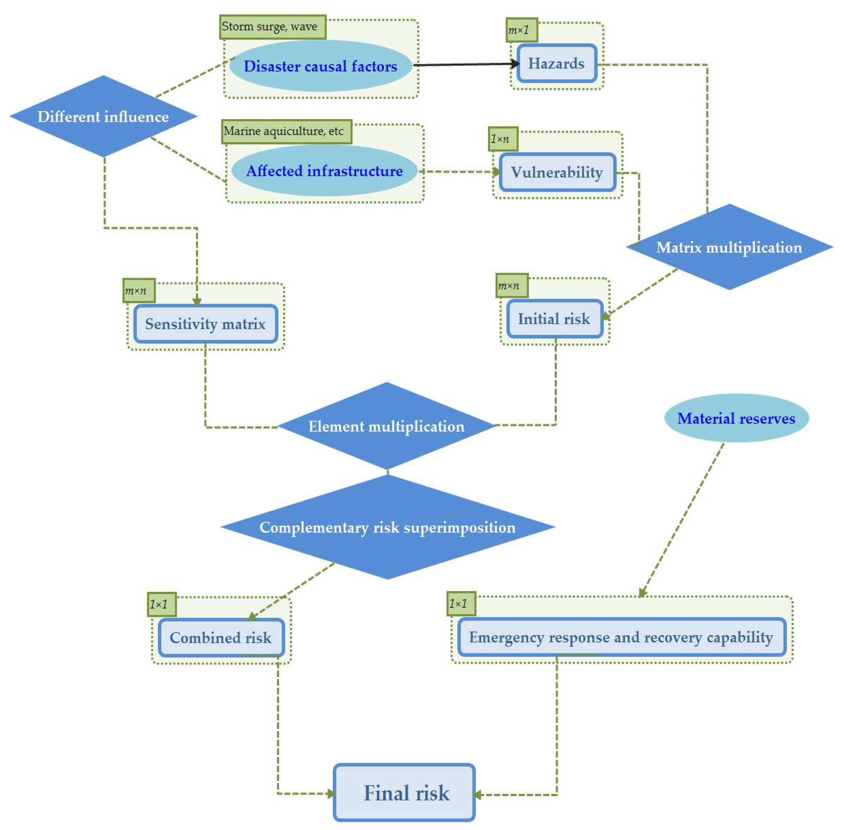
3. Risk Assessment Framework
3.1. Risk Assessment
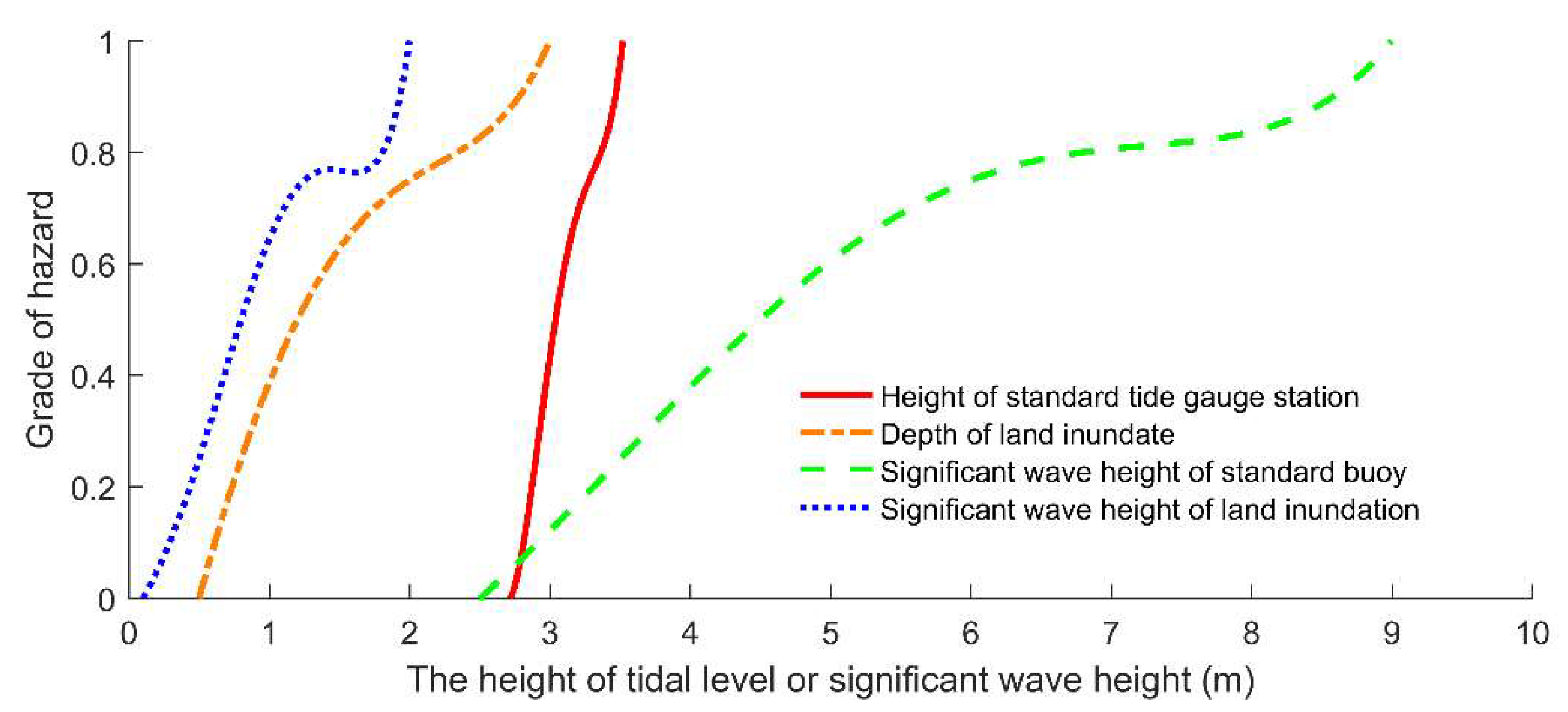
3.2. Hazard
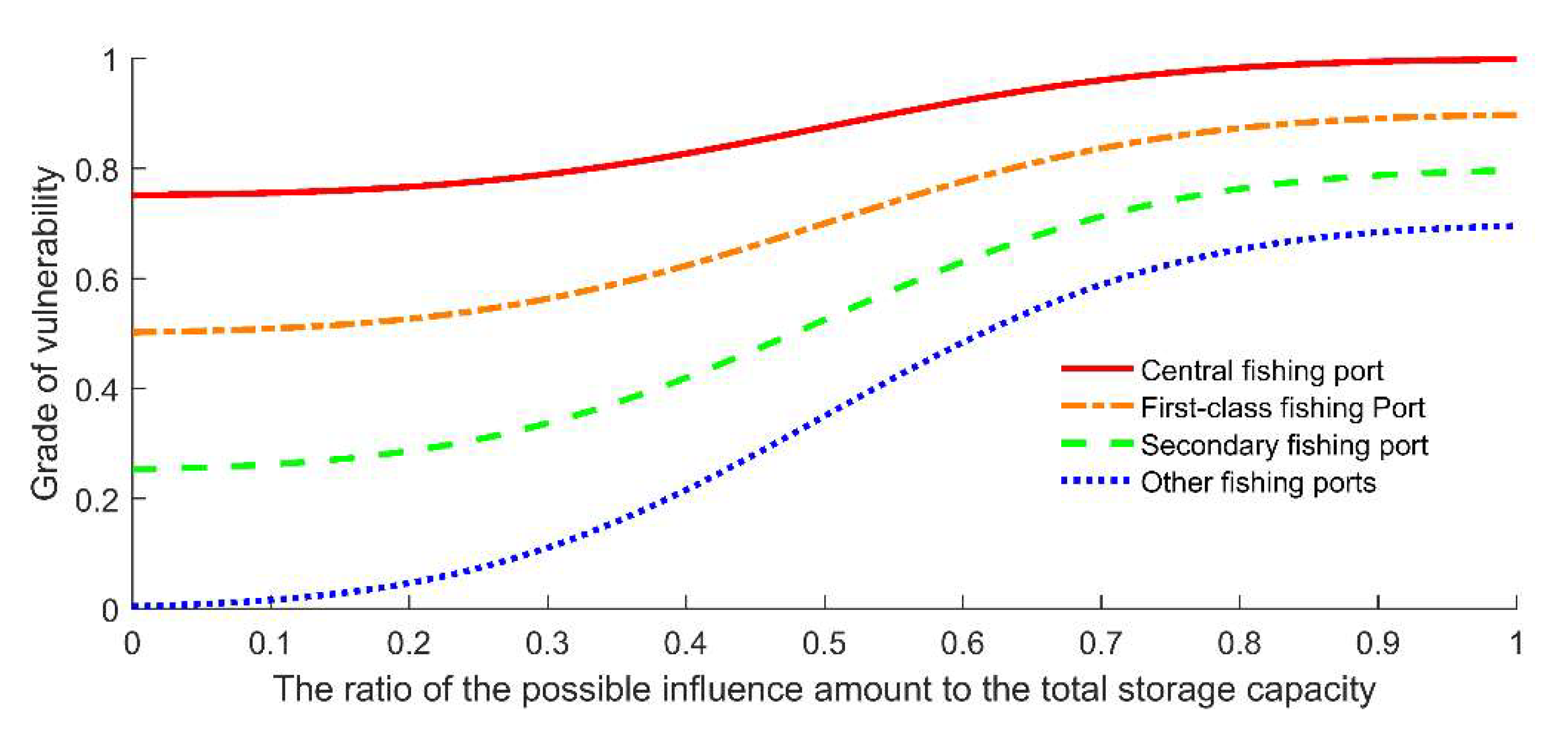
3.3. Vulnerability
3.4. Sensitivity Matrix
3.5. Emergency Response and Recovery Capability
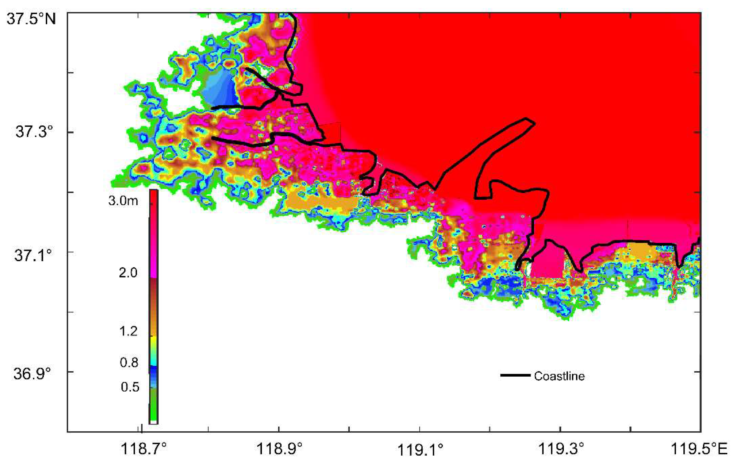
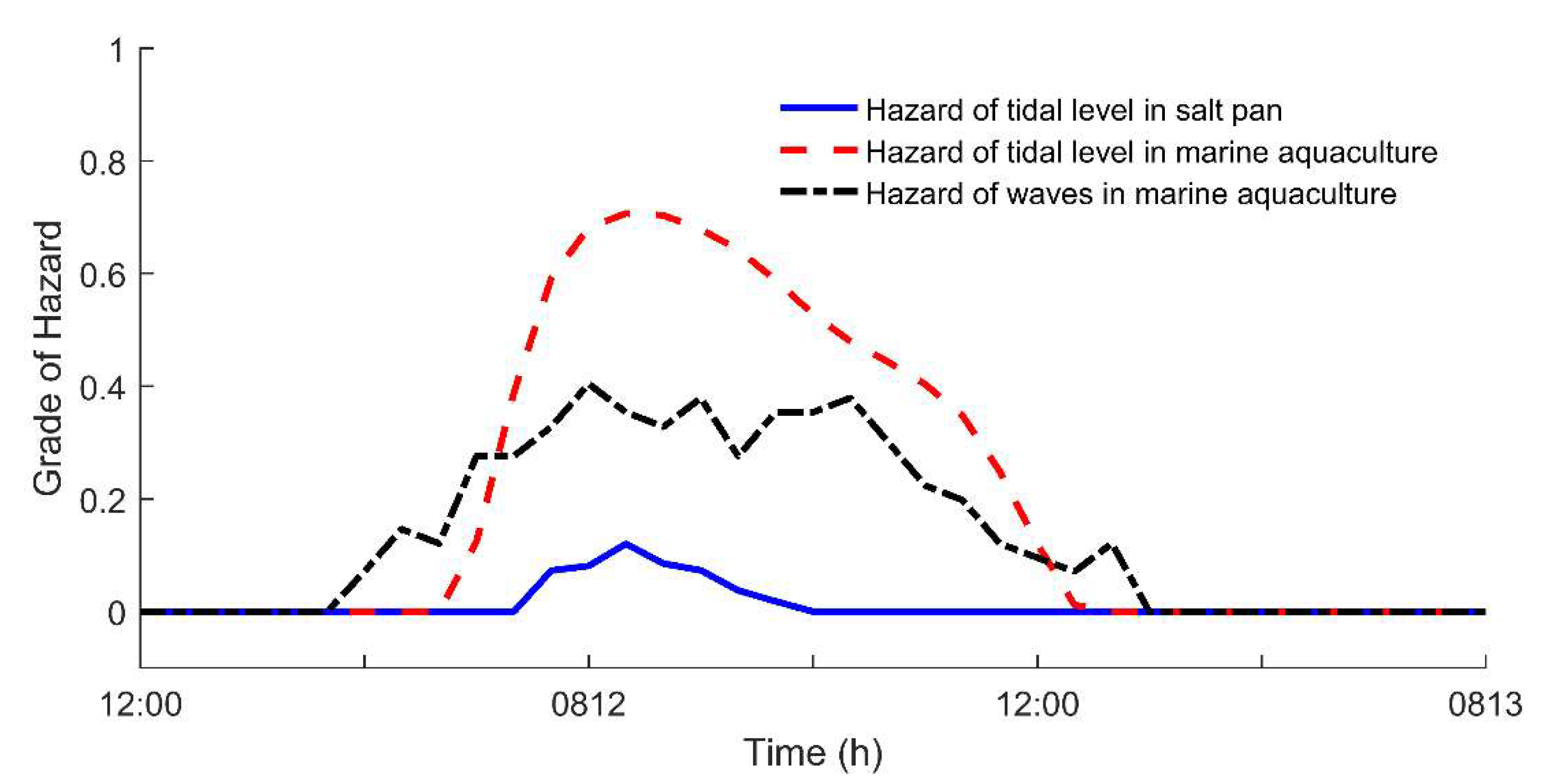
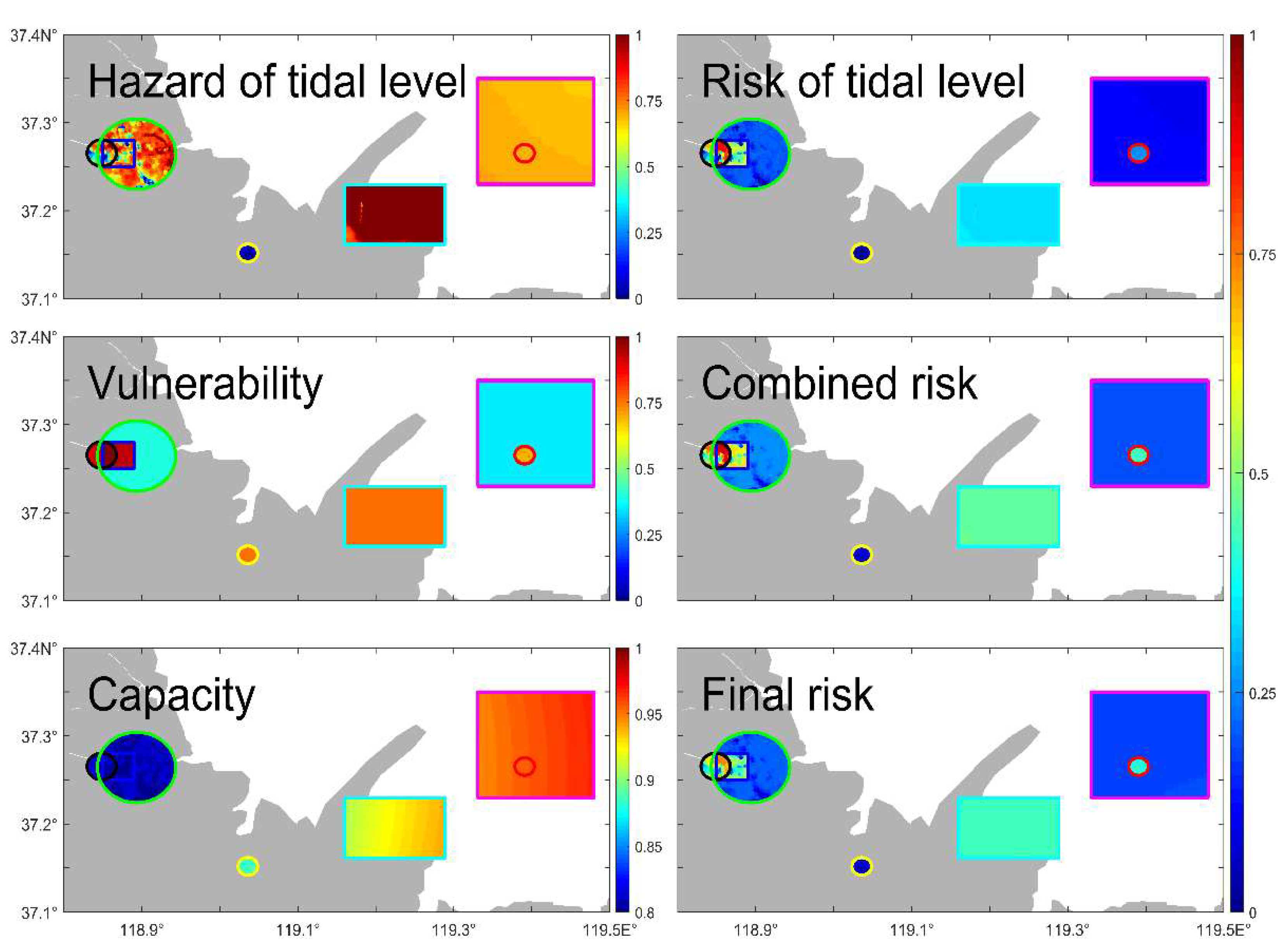
4. Risk Assessment for Typhoon Lekima Storm Surge
5. Discussion
6. Conclusions
Author Contributions
Funding
Institutional Review Board Statement
Informed Consent Statement
Data Availability Statement
Acknowledgments
Conflicts of Interest
References
- Hou, Y.; Jiang, X.; Liu, Y. China coastal seas under severe sea state: Remote sensing and dynamics studies. Chin. J. Oceanol. Limnol. 2015, 33, 1101–1103. [Google Scholar] [CrossRef]
- Nordstrom, K.F. Beaches and Dunes of Developed Coasts; Cambridge University: Cambridge, UK, 2000; pp. 165–191. [Google Scholar] [CrossRef]
- Blake, E.S.; Rappaport, E.N.; Landsea, C.W.; Miami, N. The Deadliest, Costliest, and Most Intense United States Tropical Cyclones from 1851 to 2006 (and Other Frequently Requested Hurricane Facts); Hurricanes preparedness facing the reality of more & bigger storms; NOAA/National Weather Service, National Centers for Environmental Prediction, National Hurricane Center: Miami, FL, USA, 2007. [Google Scholar] [CrossRef]
- Pielke, R.A. Normalized hurricane damage in the United States: 1900–2005. Nat. Hazards Rev. 2008, 9, 29–42. [Google Scholar] [CrossRef]
- Rey, W.; Mendoza, E.T.; Salles, P.; Zhang, K.; Teng, Y.C.; Trejo-Rangel, M.A.; Franklin, G.L. Hurricane flood risk assessment for the Yucatan and Campeche State coastal area. Nat. Hazards 2019, 96, 1041–1065. [Google Scholar] [CrossRef]
- Shi, X.; Tan, J.; Guo, Z.; Liu, Q. A review of risk assessment of storm surge disaster. Adv. Earth Sci. 2013, 28, 866–874. [Google Scholar]
- Glahn, B.; Taylor, A.; Kurkowski, N.; Shaffer, W.A. The role of the SLOSH model in National Weather Service storm surge forecasting. Natl. Weather Dig. 2009, 33, 3–14. [Google Scholar]
- Watson, C.C. The arbiter of storms: A high resolution, GIS based system for integrated storm hazard modeling. Natl. Weather Dig. 1995, 20, 2–9. [Google Scholar]
- Shepard, C.C.; Agostini, V.N.; Gilmer, B.; Allen, T.; Stone, J.; Brooks, W.; Beck, M.W. Assessing future risk: Quantifying the effects of sea level rise on storm surge risk for the southern shores of Long Island, New York. Nat. Hazards 2012, 60, 727–745. [Google Scholar] [CrossRef]
- Ferreira, Ó.; Paolo, C.; Clara, A.; Yann, B. Coastal storm risk assessment in europe: Examples from 9 study sites. J. Coast. Res. 2009, 25, 1632–1636. [Google Scholar]
- Kleinosky, L.R.; Yarnal, B.; Fisher, A. Vulnerability of Hampton Roads, Virginia to storm-surge flooding and sea-level rise. Nat. Hazards 2007, 40, 43–70. [Google Scholar] [CrossRef]
- Tsunami and Storm Surge Research Association. Tsunami and Storm Surge Hazard Map Manual; Cabinet Office of Japan: Tokyo, Japan, 2004. Available online: https://www.pwri.go.jp/icharm/publication/pdf/2004/tsunami_and_storm_surge_hazard_map_manual.pdf (accessed on 16 January 2022).
- Liu, Q.; Ruan, C.; Zhong, S.; Li, J.; Yin, Z.; Lian, X. Risk assessment of storm surge disaster based on numerical models and remote sensing. Int. J. Appl. Earth Obs. Geoinf. 2018, 68, 20–30. [Google Scholar] [CrossRef]
- Liu, Y.; Lu, C.; Yang, X.; Wang, Z.; Liu, B. Fine-scale coastal storm surge disaster vulnerability and risk assessment model: A case study of Laizhou Bay, China. Remote Sens. 2020, 12, 1301. [Google Scholar] [CrossRef]
- Kobyliński, L. Stability of ships: Risk assessment due hazards created by forces of the sea. Arch. Civ. Mech. Eng. 2008, 8, 37–45. [Google Scholar] [CrossRef]
- Quinn, N.; Lewis, M.; Wadey, M.P.; Haigh, I.D. Assessing the temporal variability in extreme storm-tide time series for coastal flood risk assessment. J. Geophys. Res. Ocean. 2014, 119, 4983–4998. [Google Scholar] [CrossRef]
- Zachry, B.C.; Booth, W.J.; Rhome, J.R.; Sharon, T.M. A national view of storm surge risk and inundation. Weather Clim. Soc. 2015, 7, 109–117. [Google Scholar] [CrossRef]
- Kameshwar, S. Multi-hazard Fragility, Risk, and Resilience Assessment of Select Coastal Infrastructure (Doctoral dissertation). In Retrieved from Rice Scholarship; Rice University: Houston, TX, USA, 2017; Available online: https://scholarship.rice.edu/handle/1911/96101 (accessed on 16 January 2022).
- Gill, J.C.; Malamud, B.D. Anthropogenic processes, natural hazards, and interactions in a multi-hazard framework. Earth-Sci. Rev. 2017, 166, 246–269. [Google Scholar] [CrossRef]
- Xu, H.; Xu, K.; Bin, L.; Lian, J.; Ma, C. Joint risk of rainfall and storm surges during typhoons in a coastal city of Haidian Island, China. Int. J. Environ. Res. Public Health 2018, 15, 1377. [Google Scholar] [CrossRef]
- Mo, D.; Hou, Y.; Li, J.; Liu, Y. Study on the storm surges induced by cold waves in the Northern East China Sea. J. Mar. Syst. 2016, 160, 26–39. [Google Scholar] [CrossRef]
- Lewis, M.; Horsburgh, K.; Bates, P.; Smith, R. Quantifying the uncertainty in future coastal flood risk estimates for the U.K. J. Coast. Res. 2011, 27, 870–881. [Google Scholar] [CrossRef]
- Pugh, D. Changing Sea Levels: Effects of Tides, Weather and Climate; Cambridge University Press: Cambridge, UK, 2004. [Google Scholar]
- Zhang, F.; Li, M. Impacts of ocean warming, sea level rise, and coastline management on storm surge in a semienclosed bay. J. Geophys. Res. Ocean. 2019, 124, 6498–6514. [Google Scholar] [CrossRef]
- Ruggiero, P. Is the intensifying wave climate of the U.S. Pacific Northwest increasing flooding and erosion risk faster than sea-level rise? J. Waterw. Port Coast. Ocean Eng. 2013, 139, 88–97. [Google Scholar] [CrossRef]
- Wahl, T.; Plant, N.G.; Long, J.W. Probabilistic assessment of erosion and flooding risk in the northern Gulf of Mexico. J. Geophys. Res. Ocean. 2016, 121, 3029–3043. [Google Scholar] [CrossRef]
- Stockdon, H.F.; Thompson, D.M.; Plant, N.G.; Long, J.W. Evaluation of wave runup predictions from numerical and parametric models. Coast. Eng. 2014, 92, 1–11. [Google Scholar] [CrossRef]
- Gumbel, E.J. Statistics of Extremes; Columbia University Press: New York, NY, USA, 1958. [Google Scholar]
- Coles, S. An Introduction to Statistical Modeling of Extreme Values; Springer: London, UK, 2001. [Google Scholar]
- Walton, T.L. Distributions for storm surge extremes. Ocean Eng. 2000, 27, 1279–1293. [Google Scholar] [CrossRef]
- Gumbel, E.J. The return period of flood flows. Ann. Math. Stat. 1941, 12, 163–190. [Google Scholar] [CrossRef]
- Warren, I.R.; Bach, H.K. MIKE 21: A modelling system for estuaries, coastal waters and seas. Environ. Softw. 1992, 7, 229–240. [Google Scholar] [CrossRef]
- Dinh, Q.; Balica, S.; Popescu, I.; Jonoski, A. Climate change impact on flood hazard, vulnerability and risk of the Long Xuyen Quadrangle in the Mekong Delta. Int. J. River Basin Manag. 2012, 10, 103–120. [Google Scholar] [CrossRef]
- Sharifi, F.S.; Ezam, M.; Khaniki, A.K. Evaluating the results of hormuz strait wave simulations using WAVEWATCH-III and MIKE21-SW. Int. J. MArine Sci. Eng. 2012, 2, 163–170. [Google Scholar]
- Wang, J.; Xu, S.; Ye, M.; Huang, J. The MIKE model application to overtopping risk assessment of seawalls and levees in Shanghai. Int. J. Disaster Risk Sci. 2011, 2, 32–42. [Google Scholar] [CrossRef][Green Version]
- Danish Hydraulic Institute. MIKE 21 Coastal Hydraulics and Oceanography, Hydrodynamic Module, Reference Manual; DHI Water and Environment: Hørsholm, Denmark, 2008. [Google Scholar]
- Panigrahi, J.K.; Tripathy, J.K.; Murty, A. Extremity analysis of storm surge for fixing safe design water level. Nat. Hazards 2011, 56, 347–358. [Google Scholar] [CrossRef]
- Kong, X.; College, S.E.; University, D.M. A numerical study on the impact of tidal waves on the storm surge in the north of liaodong bay. Acta Oceanol. Sin. 2014, 33, 35–41. [Google Scholar] [CrossRef]
- Siahsarani, A.; Khaniki, A.K.; Bidokhti, A.A.; Azadi, M. Numerical modeling of tropical cyclone-induced storm surge in the gulf of oman using a storm surge–wave–tide coupled model. Ocean Sci. J. 2021, 56, 1–16. [Google Scholar] [CrossRef]
- Li, J.; Hou, Y.; Mo, D.; Liu, Q.; Zhang, Y. Influence of tropical cyclone intensity and size on storm surge in the Northern East China Sea. Remote Sens. 2019, 11, 3033. [Google Scholar] [CrossRef]
- Moon, I.J.; Ginis, I.; Hara, T. Impact of the reduced drag coefficient on ocean wave modeling under hurricane conditions. Mon. Weather Rev. 2008, 136, 1217–1223. [Google Scholar] [CrossRef]
- Powell, M.D.; Vickery, P.J.; Reinhold, T.A. Reduced drag coefficient for high wind speeds in tropical cyclones. Nature 2003, 422, 279–283. [Google Scholar] [CrossRef]
- Oey, L.Y.; Ezer, T.; Wang, D.P.; Fan, S.J.; Yin, X.Q. Loop Current warming by hurricane Wilma. Geophys. Res. Lett. 2006, 33, L08613. [Google Scholar] [CrossRef]
- Maskrey, A. Disaster Mitigation: A Community Based Approach; Oxfam: Oxford, UK, 2019. [Google Scholar]
- Bronstert, A. Floods and climate change: Interactions and impacts. Risk Anal. 2013, 23, 545–557. [Google Scholar] [CrossRef]
- Plate, E.J. Flood risk and flood management. J. Hydrol. 2002, 267, 2–11. [Google Scholar] [CrossRef]
- Tingsanchali, T.; Karim, M.F. Flood hazard and risk analysis in the southwest region of Bangladesh. Hydrol. Processes 2005, 19, 2055–2069. [Google Scholar] [CrossRef]
- Merz, B.; Hall, J.; Disse, M.; Schumann, A. Fluvial flood risk management in a changing world. Nat. Hazards Earth Syst. Sci. 2010, 10, 509–527. [Google Scholar] [CrossRef]
- UNISDR. 2009 UNISDR-Terminology on Disaster Risk Reduction; UNISDR: Geneva, Switzerland, 2009; Available online: https://www.undrr.org/publication/2009-unisdr-terminology-disaster-risk-reduction (accessed on 16 January 2022).
- Blaikie, P.; Cannon, T.; Davis, I.; Wisner, B. At Risk: Natural Hazards, People’s Vulnerability and Disasters; Routledge: London, UK, 1994. [Google Scholar]
- Liu, Q.; Li, J.; Ruan, C.Q.; Yin, Z.H.; Jiao, Y.; Sun, Q.; Lian, X.H.; Zhong, S. Risk assessment and zoning of sea level rise in Shandong Province. J. Oceanol. Limnol. 2019, 37, 2014–2024. [Google Scholar] [CrossRef]
- Church, J.A.; White, N.J. A 20th century acceleration in global sea-level rise. Geophys. Res. Lett. 2015, 33, 313–324. [Google Scholar] [CrossRef]
- Haigh, I.D.; Nicholls, R.; Wells, N. A comparison of the main methods for estimating probabilities of extreme still water levels. Coast. Eng. 2010, 57, 838–849. [Google Scholar] [CrossRef]
- Michele, C.D.; Salvadori, G.; Passoni, G.; Vezzoli, R. A multivariate model of sea storms using copulas. Coast. Eng. 2007, 54, 734–751. [Google Scholar] [CrossRef]
- Zhai, J.; Yin, Q.; Dong, S. Co-occurrence probability of typhoon surges affecting multiple estuaries in the northern coastal region of Taiwan. Reg. Stud. Mar. Sci. 2020, 42, 101582. [Google Scholar] [CrossRef]
- Porcu, F.; Arago, L.; Aguzzi, M.; Valentini, A.; Sabatino, S.D. Extreme Wave Events Attribution Using ERA5 Datasets for Storm-surge Studies in the Northern Adriatic Sea; EGU2020: Munich, Germany, 2020. [Google Scholar]
- Orton, P.; Georgas, N.; Blumberg, A.; Pullen, J. Detailed modeling of recent severe storm tides in estuaries of the New York City region. J. Geophys. Res. Ocean. 2012, 117, C09030. [Google Scholar] [CrossRef]


| Name | Numerical Value | Indicator | |||
|---|---|---|---|---|---|
| Grade | 1 | 2 | 3 | 4 | Hazard Grade |
| Hazard value range | 0.75–1.00 | 0.50–0.75 | 0.25–0.50 | 0.00–0.25 | Standardize the hazard value of [0, 1]. |
| Tidal level of return period (m) | 3.28–3.52 (100–200) | 3.04–3.28 (50–100) | 2.90–3.04 (33.3–50) | 2.72–2.90 (20–33.3) | The tidal level return period is calculated based on the height of tide gauge station WFG. (The year of return period (a)) |
| Depth of inundation (m) | 2.00–3.00 | 1.20–2.00 | 0.80–1.20 | 0.50–0.80 | According to the depth of the impact on people of different ages were divided into grades (Depth of inundation refer to Tsunami and Storm Surge Research Association [12]). |
| Significant wave height of four-color alarm (m) Significant wave height of inundation (m) | 6.00–9.00 | 4.50–6.00 | 3.50–4.50 | 2.50–3.50 | Grades are divided according to the four-color alarm levels effective wave height pairs representing buoy station QF104 |
| 1.25–2.00 | 0.80–1.25 | 0.50–0.80 | 0.10–0.50 | According to the size of the waves to the different stages of human impact of the proposed classification. | |
| Name | Evidence of Division | Highest Level | High Level | Medium Level | General Level |
|---|---|---|---|---|---|
| Marine aquiculture | Breeding method | Pond culture | Mudflat culture | Cage culture | Raft culture |
| Value interval | 0.75–1 | 0.5–0.9 | 0.25–0.8 | 0–0.7 | |
| Fishing port | Fishing grades | Center fishing | First class | Second class | Other class |
| Value interval | 0.75–1 | 0.5–0.9 | 0.25–0.8 | 0–0.7 | |
| Chemical plant | Storage or not | Stored | - | - | Not |
| Value interval | 0.8–1 | - | - | 0.5–0.8 | |
| Marine ranching | Breeding ways | Pond culture | Mudflat culture | Cage culture | Raft culture |
| Value interval | 0.75–1 | 0.5–0.9 | 0.25–0.8 | 0–0.7 | |
| Salt pan | Abandoned or not | Not | - | - | Abandoned |
| Value interval | 0.5–1 | - | - | 0–0.5 | |
| Material reserves | Degree of importance | Importance | - | - | General |
| Value interval | 0.5–1 | - | - | 0–0.8 | |
| Tourist area | Slack or Busy seasons | Busy season | - | - | Slack season |
| Value interval | 0.5–1 | - | - | 0–1 |
| Marine Aquiculture | Fishing Port | Chemical Plant | Marine Ranching | Salt Pan | Material Reserves | Tourist Area | Total | |
|---|---|---|---|---|---|---|---|---|
| Relative tidal risk | 0.4 | 0.7 | 0.6 | 0.4 | 0.8 | 0.6 | 0.5 | 4 |
| Relative wave risk | 0.6 | 0.3 | 0.4 | 0.6 | 0.2 | 0.4 | 0.5 | 3 |
| Relative total risk | 1 | 1 | 1 | 1 | 1 | 1 | 1 | 7 |
| Total risk weight | 1 | 0.9 | 1.5 | 1 | 0.8 | 1 | 1.1 | 7.3 |
| Normalized matrix | 0.444 | 0.700 | 1.000 | 0.444 | 0.711 | 0.667 | 0.611 | 8.111 |
| 0.667 | 0.300 | 0.667 | 0.667 | 0.178 | 0.444 | 0.611 |
| Marine Aquiculture | Fishing Port | Chemical Plant | Marine Ranching | Salt Pan | Material Reserves | Tourist Area | |
|---|---|---|---|---|---|---|---|
| Hazard rating of tide | Height of recurrence period | Depth of land inundate | Depth of land inundate | Height of recurrence period | Depth of land inundate | Depth of land inundate | Depth of land inundate |
| Hazard rating of waves | QF104 buoy effective wave high grade replaces all hazard affecting the infrastructure, and the maximum score is 0.4042 (corresponding to 4.1 m effective wave high). | ||||||
| Type | Raft culture | Center fishing | Stored | Cage culture | Not abandoned | General | Busy season |
| Value interval | 0–0.7 | 0.75–1 | 0.8–1 | 0.25–0.8 | 0.5–1 | 0–0.8 | 0.5–1 |
| Storage ratio | 0.5 | 0.5 | 0.5 | 0.5 | 0.5 | 0.5 | 0.5 |
| Vulnerability | 0.350 | 0.875 | 0.900 | 0.525 | 0.750 | 0.400 | 0.750 |
Publisher’s Note: MDPI stays neutral with regard to jurisdictional claims in published maps and institutional affiliations. |
© 2022 by the authors. Licensee MDPI, Basel, Switzerland. This article is an open access article distributed under the terms and conditions of the Creative Commons Attribution (CC BY) license (https://creativecommons.org/licenses/by/4.0/).
Share and Cite
Li, J.; Mo, D.; Li, R.; Hou, Y.; Liu, Q. Establishing a Risk Assessment Framework for Marine Assets and Assessing Typhoon Lekima Storm Surge for the Laizhou Bay Coastal Area of the Bohai Sea, China. J. Mar. Sci. Eng. 2022, 10, 298. https://doi.org/10.3390/jmse10020298
Li J, Mo D, Li R, Hou Y, Liu Q. Establishing a Risk Assessment Framework for Marine Assets and Assessing Typhoon Lekima Storm Surge for the Laizhou Bay Coastal Area of the Bohai Sea, China. Journal of Marine Science and Engineering. 2022; 10(2):298. https://doi.org/10.3390/jmse10020298
Chicago/Turabian StyleLi, Jian, Dongxue Mo, Rui Li, Yijun Hou, and Qingrong Liu. 2022. "Establishing a Risk Assessment Framework for Marine Assets and Assessing Typhoon Lekima Storm Surge for the Laizhou Bay Coastal Area of the Bohai Sea, China" Journal of Marine Science and Engineering 10, no. 2: 298. https://doi.org/10.3390/jmse10020298
APA StyleLi, J., Mo, D., Li, R., Hou, Y., & Liu, Q. (2022). Establishing a Risk Assessment Framework for Marine Assets and Assessing Typhoon Lekima Storm Surge for the Laizhou Bay Coastal Area of the Bohai Sea, China. Journal of Marine Science and Engineering, 10(2), 298. https://doi.org/10.3390/jmse10020298