Improvement of Rudder Cavitation Performance Using Rudder Inflow Measurements in Large Cavitation Tunnel

Abstract

One of the important things in a ship’s rudder design is the incidence angle of the rudder inflow to improve rudder cavitation performance. In the present study, the rudder inflow is measured by a 3-D LDV (laser Doppler velocimetry) system in a large cavitation tunnel, where the ship model tests are performed at a rather high Reynolds number of 10⁷~10⁸. Through the evaluation of the transverse velocity component using water injection experiments in the test section, the reliability of the 3-D LDV measurements is confirmed. The three-dimensional velocity components of rudder inflow between the rudder and propeller are successfully measured and are compared with numerical simulation results to see good agreement. The incidence angle distribution of the rudder inflow is obtained from the 3-D velocity components and shows a large angle at the range of 0.5 < Z/Span < 0.9, where the cavitation mainly occurred. The asymmetry-type rudder proposed based on rudder inflow measurements showed outstanding improvement of cavitation performance, compared with the flat-type rudder.

1. Introduction

The rudder provides a ship with directional stability, maneuverability, and control performance. The rudder of a ship is typically placed behind the propeller to increase the efficiency of the maneuver. In particular, ship rudders are affected by complex hydrodynamics depending on the hull, inclined shaft, V-strut, and propeller operation. In accordance with the recent trend of increasing the size of the ship and increasing the required horsepower, the velocity of flow coming into the propeller and rudder is greatly increased, and a rudder shape that can withstand high fluid loads is required.

For naval vessels, full-spade rudders are used, and semi-spade rudders (Figure 1) are widely applied for general merchant ships. Cavitation occurs on the rudder because the fluid moving along the rudder surface locally lowers its pressure below the vapor pressure of water, so that the fluid boils and gas is generated. Cavitation appears in various forms depending on the surrounding hydrodynamic environments, and when the cavitation strongly collapses, it causes severe erosion on the rudder’s surface. 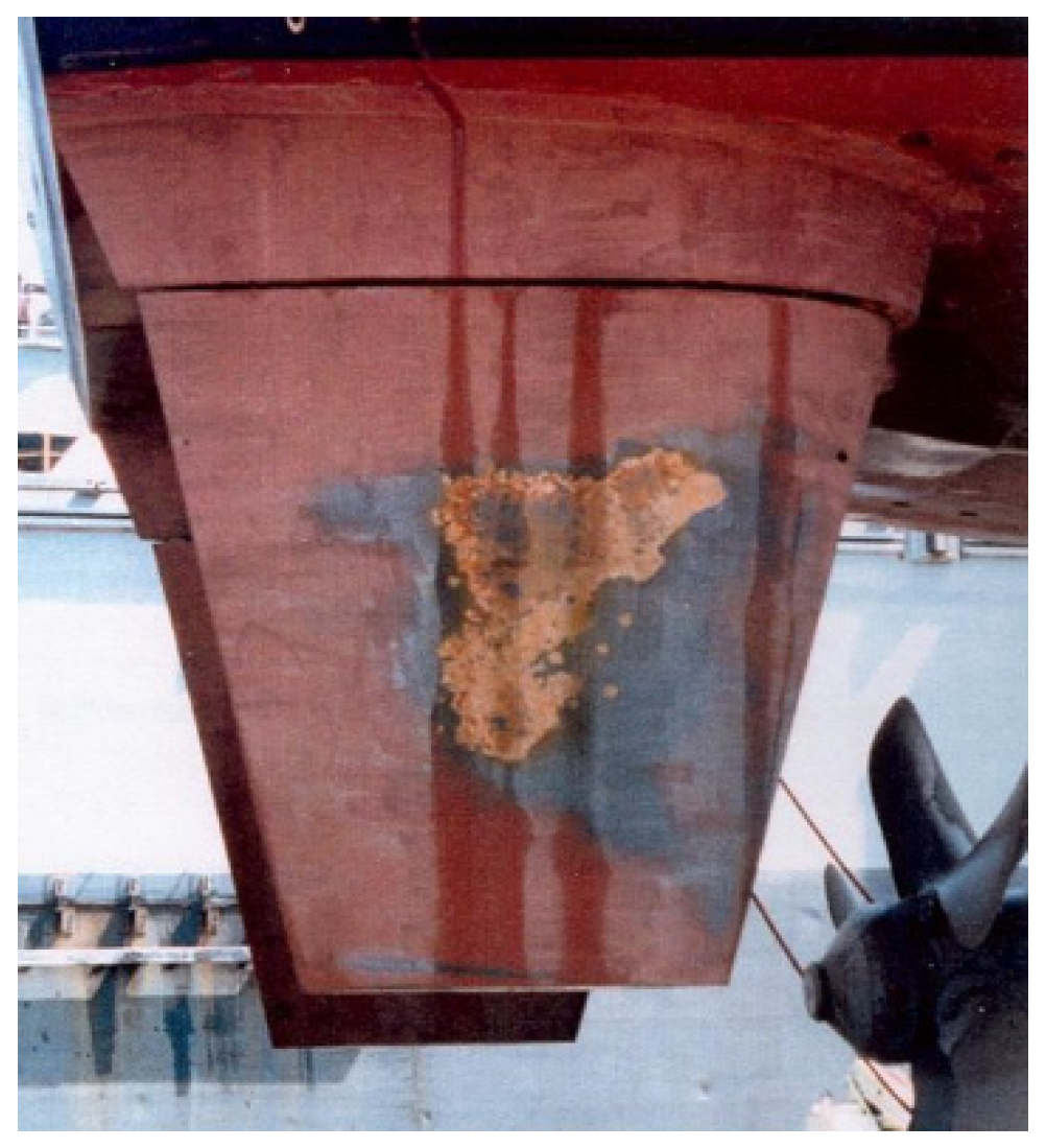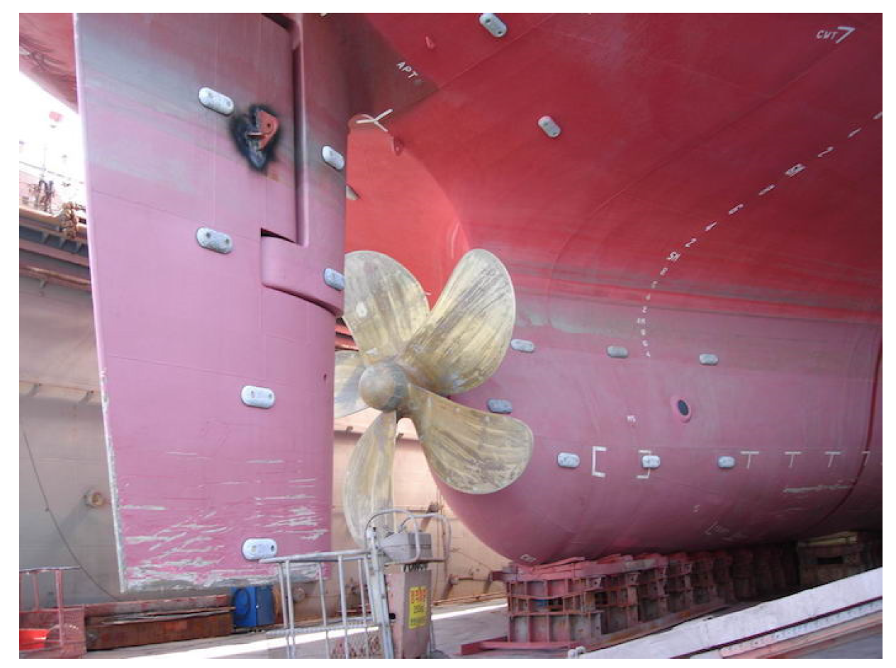Figure 2 shows the erosion that occurred on the full-spade rudder of a navy vessel. Rudder cavitation seriously erodes the surface of the rudder, greatly increasing the maintenance cost of the rudder and adversely affecting the operation schedule of the ship. A more serious problem is that cavitation generated from the rudder may cause serious vibrations or noises, exposing a fatal weakness in anti-submarine operations. In addition, since the cavitation generated from the rudder may cause an increase in drag, which means the resistance of the ship itself, it is considered very important to study a rudder design that can improve the cavitation performance of the rudder.

One of the most important factors for rudder design is information on the incidence angle (angle of attack) of the rudder inflow. When the incidence angle of the rudder inflow is excessive, strong cavitation due to high fluid loads occurs on the rudder surface, which increases the possibility of erosion and noise.

Shen et al. [1] studied the effects of ship hull and propeller on rudder cavitation at the US Navy’s Large Cavitation Channel and measured the rudder inflow angles in the propeller slipstream by a two-component LDV system. They employed a very special LDV system where the optical path was set inside a ship model. Three-component velocity components were non-coincidently obtained by two LDV configurations to determine the rudder inflow angle information.

Chesnakas and Jessup [2] examined the behavior of tip-vortex flow of the propeller by two different LDV systems of 2-component and 1-component in a 36-inch water tunnel. The three-component velocity components were successfully measured in random mode or in coincidence mode. They presented the tip-vortex structure and the variation of this structure with advanced coefficient and location.

Felli et al. [3] measured the flows around a full-spade rudder in the medium-sized cavitation tunnel without any ship model. Felli et al. have used two LDV configurations on the top and side windows to obtain the transverse velocity components of the propeller-induced wake. Although three-component velocities were successfully combined by the two-component LDV system and two configurations, they were not applied, coincidently.

Paik et al. [4] measured the incidence angle of the rudder inflow in a medium-sized cavitation tunnel using a 2-D PIV (particle image velocimetry) technique. However, as it was measured in the absence of a ship model, the flow around the rudder could not be a real one. In the case of a large cavitation tunnel, it is easy to simulate the actual flow behaviors by installing ship, propeller, and rudder models together.

In past LDV experiments conducted in the cavitation tunnel, three velocity components could not be measured simultaneously, but two velocity components and one velocity component were measured separately. Transverse (lateral) velocity component could be obtained only using the synthesis method with two- and one-velocity components. However, in the present study, since three velocity components were simultaneously measured using the 3-D LDV, the transverse velocity component could be obtained without any synthesis method, and the accuracy of the transverse velocity component was improved. To verify the accuracy of it, a separate water jet test was additionally performed.

Since the hydrodynamic performance of a rudder is largely determined by the in-flow of the propeller operating in the wake of the hull, a detailed understanding of hull-propeller-rudder interaction flows is required.

Simonsen [5] applied computational fluid dynamics (CFD) to investigation of the interaction effects of hull–propeller–rudder on the maneuvering performance of a tanker ship. In his research, the hull-on-propeller and hull-on-rudder interactions were examined through depicting the local flow features and the rudder-on-hull interaction was estimated by using the local and global rudder forces. In his investigation of the propeller-on-rudder interaction, the propeller was not modeled directly in the CFD code but treated as a body-force concept.

Kaijia [6] proposed a numerical approach to optimize the interaction between a ship hull, a propeller, and a rudder by use of numerical simulations. A Reynolds averaged Navier–Stokes (RANS)-method-based CFD software was used for the viscous flow analyses, in which a potential flow method was utilized to consider the influences of the propeller. The changes in propeller characteristics in various configurations of hull–propeller–rudder were analyzed including hull resistance and self-propulsion factors. A similar numerical approach, a RANS solver coupled with a body force method to consider the effects of propeller rotation, was studied by Lungu and Pacuracu [7]. The main objective of their research was to investigate the flow characteristics around a maneuvering ship, and in particular, to analyze the performance of the propeller due to the asymmetric inflows in various maneuvering conditions. Villa et al. [8] numerically investigated the propeller–rudder interactions. The study focused on the rudder forces varying the propulsion loading conditions and relative position between the propeller and rudder. They used an open-source CFD solver with an actuator disk theory for propeller forces. Xie and Zhang [9] carried out numerical simulations to estimate the resistance change of a VLCC ship considering the hull–propeller–rudder interaction. They used the vortex lattice method (VLM) to reproduce propeller forces and distributed these forces on the propeller area in the viscous solver grid. Sanada et al. [10] experimentally and numerically investigated the hull–propeller–rudder interaction of a container ship in circular motions by decomposing the forces of the hull, propeller, and rudder into each contribution. Unlike the straight advancing situation, in circular motions, the development of strong hull vortices and the interaction between the propeller and the rudder increased. Mascio et al. [11] analyzed the vortex–rudder interaction in detail by the propeller within the range of RANS flows, where the rotation of the propeller was solved by a dynamic overlapping meshing algorithm. Yang et al. [12] investigated the hydrodynamic performance of a semi-spade rudder operating at different advance coefficients of the propeller. They tested the dependence of RANS-based turbulence models on the propeller–rudder interaction in terms of integral forces and local flows. Bekhit et al. [13] carried out the numerical simulations of a ship model advancing in calm water to study on the hull–propeller and hull–propeller–rudder interaction. A RANS-based flow solver with the sliding mesh technique for propeller rotation was used to predict the variation of resistance and thrust forces and wake flow for the ship with and without a rudder.

Through the above literature reviews, the validity of the RANS method applied to hull–propeller–rudder interaction problems was confirmed. In addition, it should be noted that the rotation flow of the propeller must be directly analyzed using dynamic mesh techniques in order to precisely analyze the interaction flow. With reference to these previous research works, the current numerical analyses considered the full appended ship model installed in the cavitation tunnel for mesh generation and directly solved the propeller flow using the sliding mesh method applied to the propeller.

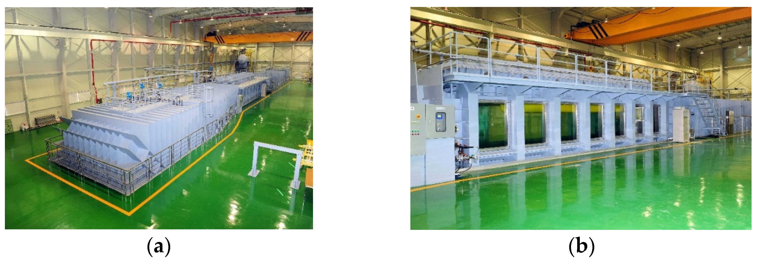
KRISO (Korea Research Institute of Ships and Ocean Engineering, formerly MOERI) constructed an LCT (large cavitation tunnel) in 2009 to observe the ship cavitation and assess its performance. LCT has the test section dimension of 2.8^W × 1.8^H × 12.5^L m³ and gives a maximum flow speed of 16.5 m/s. Figure 3 shows the photos of the upper structure in LCT. LCT is able to provide a more realistic 3-D wake of the propeller in the condition of high Reynolds number regime (10⁷~10⁸), which is close to the full-scale Reynolds number [14]. To investigate and visualize the flow around the ship model, arranged in LCT’s test section, flow measurement technologies such as Pitot tube, LDV, and PIV could be employed. Pitot tube is considered to be not appropriate in LCT because very strong structural strength or reinforcement in its housing/strut are required to prevent any damages caused by flow disturbance on the measurement system. In the case of PIV, as lots of seeding particles need to be mixed with as much water as 2350 tons in LCT, the process of cleaning before the cavitation observation test costs too much expense and time. Moreover, PIV is not a good option for measuring the flows between the ship hull and propeller, and the flow around the rudder because of the difficulty in light sheet illumination. LDV is a good option against the measurement regions of narrow space and difficult laser illumination because it is the pointwise measurement technique. Thus, the 3-D LDV system (provided by Dantec Dynamics), positioned outside the test section, was prepared in LCT [15].

In the present study, the Cartesian velocity components of the rudder inflow between a propeller and a rudder were coincidently measured to extract the incident angle data, and they were compared with the results obtained by numerical simulation to see the feasibility of the 3-D LDV measurements. The rudder incidence angle distribution on the flat-type rudder provides good information for the design of the asymmetry-type rudder. Eventually, the cavitation performance of the asymmetry-type rudder was compared with that of the flat-type rudder.

2. The 3-D LDV System

Many of the experiments in LCT have been conducted for surface ship models, which were normally arranged close to the wave suppression plate as in Figure 4. It is difficult to measure the flows around the propeller or rudder model by using a general type of 3-D LDV because it is located near the wave suppression plate. For the successful measurement of flow, the 3-D LDV system was established as in

Table 1. Specification of the 3-D LDV system.

Item	Value
Wave length (nm)	514 (green), 488 (blue), 532 (yellow)
Focal length (mm)	1600
Beam expander ratio	1.5
Beam spacing (mm)	250
Beam diameter (mm)	4.1
Control volume size (mm)	dx = 0.23, dy = 0.23, dz = 4.42

, arranging the probes as shown in Figure 5.

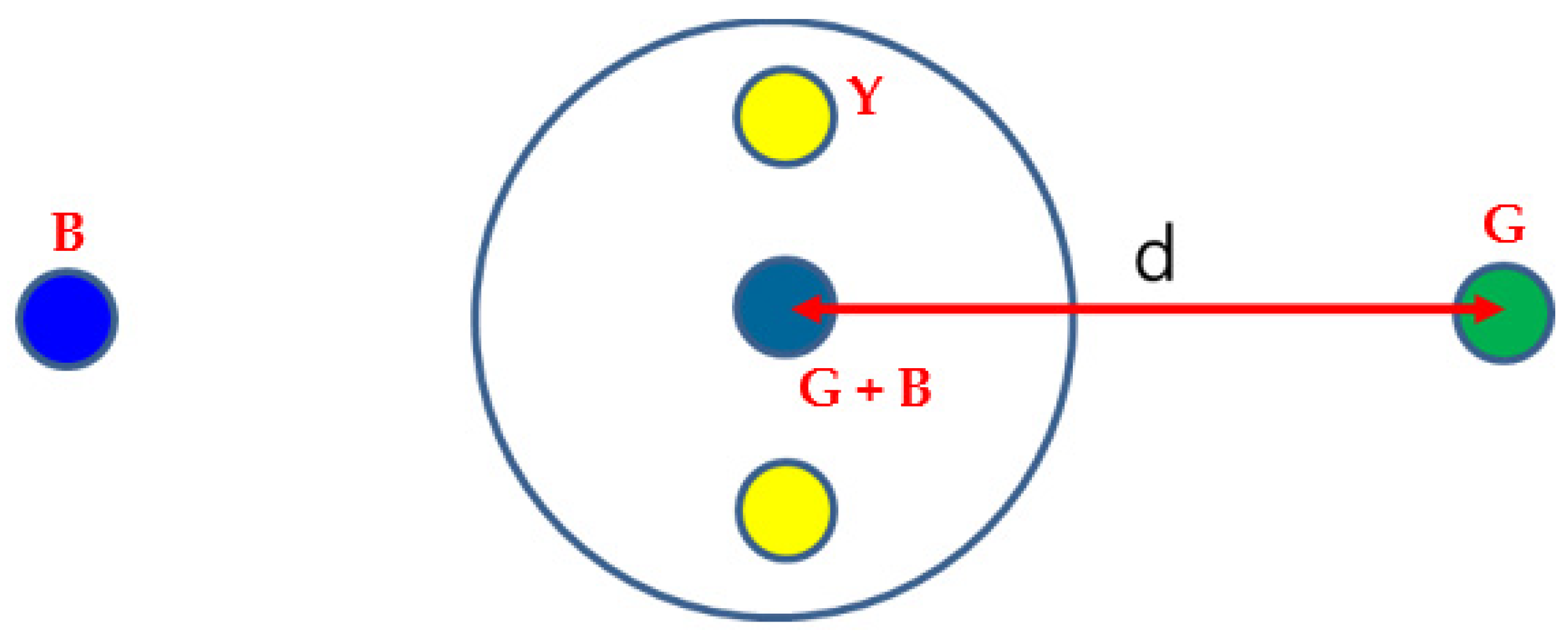
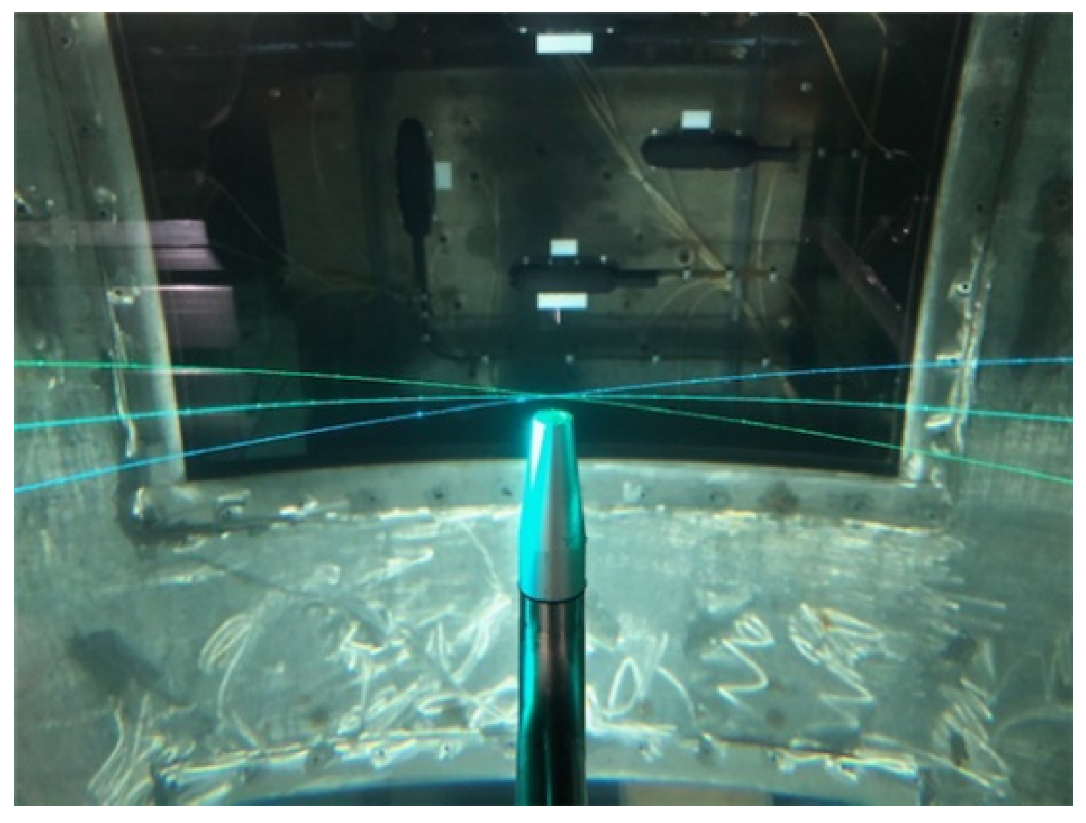
The two-dimensional velocity components in the horizontal plane were obtained by the green and blue beams located at the horizontal frame. The center beam was formed by combining green and blue beams together. The vertical velocity component was measured by a pair of yellow beams. The 3-D probe was located in the air outside the test section, and the incident beams went to the test section through an acrylic window of 100 mm thickness. The calibration procedure was necessary because the acrylic window caused refraction of the beam paths. We arranged three DPSS (diode-pumped solid state) lasers for the 3-D LDV system as in Figure 6, to provide enough power to each beam and to receive sound Doppler signals. The DPSS laser system adopted an additional yellow beam and supplied 150–200 mW power to each beam equally.

The surface of an acrylic side window in the test section was not exactly uniform because it was affected by the variation of the tunnel’s static pressure and flow velocity, and its border was fixed firmly to the tunnel window’s frame. If the surface of the window was not uniform but deformed slightly, the calibration process was so difficult to focus beams on the pin hole inside the test section. Thus, we prepared a CCD chip (provided by Dantec Dynamics) for the calibration of the 3-D LDV in the still water. The spatial resolution of the CCD chip was 1024 × 800 pixels and its pixel pitch was 10 μm. The CCD chip was extended by a long strut from the tunnel top and was connected to a laptop computer to see the beam spots on the screen. Three beams except two yellow beams were adjusted to square their waist with that of the reference main beam by finely tuning the optical controller. In the meantime, the intensity of each beam should be lowered sufficiently to avoid damage to the CCD chip.

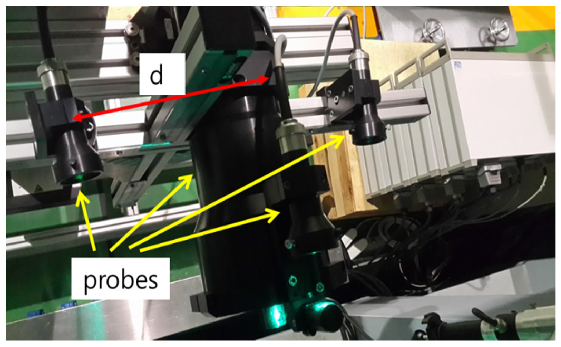
The probe spacing for the 3-D LDV system (Figure 7) was d = 250 mm. The uncertainty analysis for mean velocities was conducted at the condition of uniform flow of 9.0 m/s in the empty test section. The uncertainties in mean were 0.072% (U), 0.082% (V), and 0.081% (W). Here, U, V, and W are flow velocities in the X-, Y-, and Z-directionals, respectively. The side acrylic windows have the dimension of 1.0 × 1.3 × 0.1 m³ to conveniently observe the model in the test section. As the thickness of the window is increased, it becomes more difficult to form uniform polarization and thickness distribution on the acrylic material. The locally ununiformed polarization and thickness distribution may cause different refraction of the laser beams and deform the Doppler signal, reducing the data rate and reliability of the measurements. In the present study, we installed a rather uniform window in the test section regarding polarization and thickness, but we found that the data rate was abruptly reduced when the measurement position departed from the calibration position as much as ±150 mm.

3. Verification of the Transverse Velocity Component in the 3-D LDV System

Conventionally, a rotating disk was mainly used to verify the axial flow velocity of fluid measured by the LDV system. With the rotating disk connected to the motor, the focus of the LDV laser beams is placed on the surface of the disk and the number of motor rotations is adjusted to determine the surface velocity of the disk; thus, the velocity calibration can be made by comparing it with the velocity measured by the LDV system. However, since the verification of the transverse (Y-directional) flow velocity is not possible with the rotating disk, a separate device capable of verifying the current transverse velocity is required when the laser beams are illuminated in the transverse direction in the cavitation tunnel.

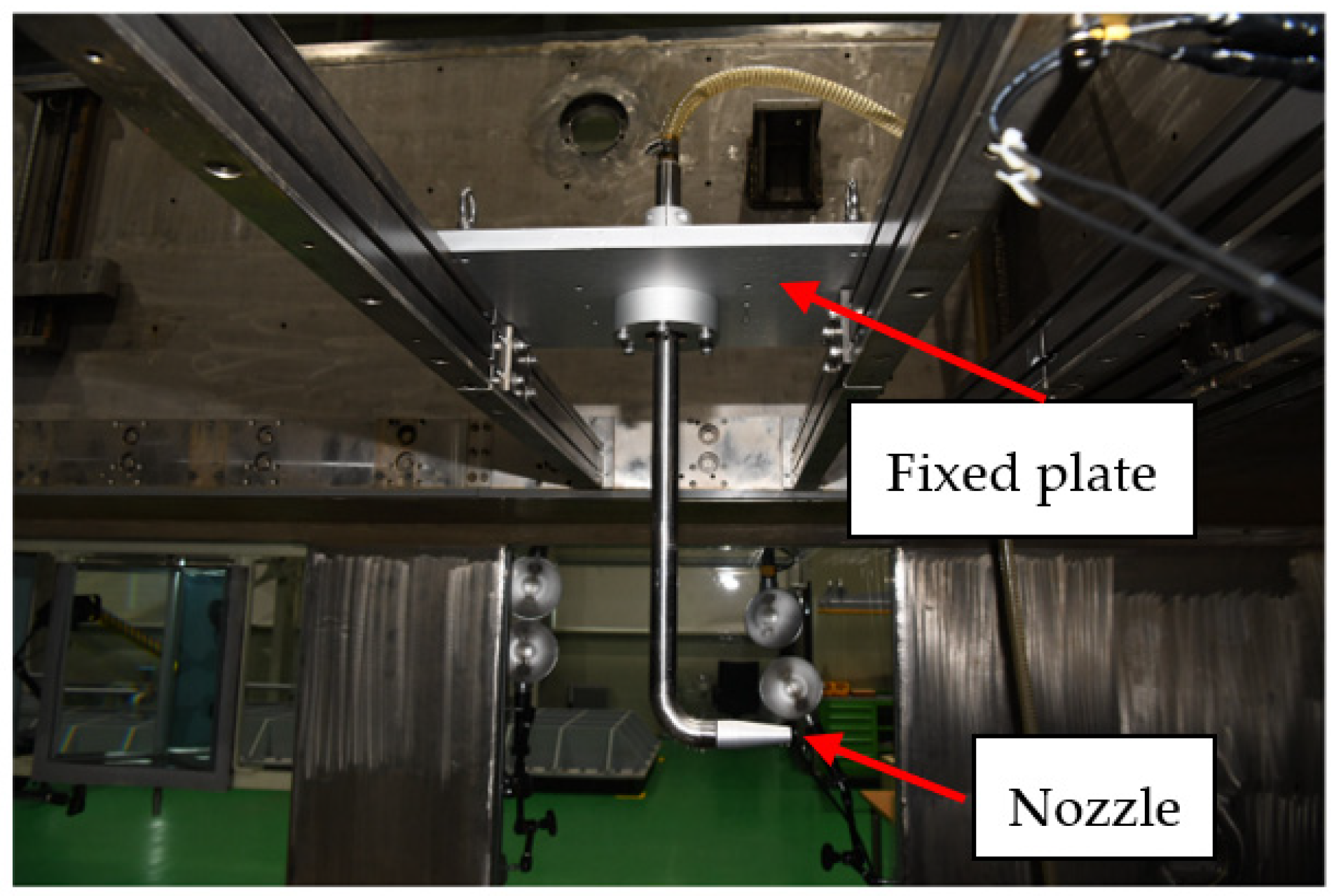
The device for the verification of transverse velocity component in the 3-D LDV measurement includes a fixed plate, a water injection unit and an angle adjusting device, as shown in Figure 8. It may also be configured to additionally include a water pump and a flow control device. The fixed plate is installed on the upper window of the cavitation tunnel test section to support the water injection unit.

The water injection unit serves to inject water at a position adjacent to the focal point of the laser beams inside the test section. A water inlet port for injecting water supplied by a pump is provided at an upper portion of the water injection unit, and a water injection nozzle is provided at the lower portion. The angle of the water injection nozzle can be changed clockwise or counterclockwise by an angle adjustment device. Figure 9 shows that the focus formed by a three-color laser beams is located at a location adjacent to the water outlet of the water injection nozzle. The water injection nozzle in Figure 9 is positioned to face the longitudinal direction of the cavitation tunnel (the angle change is 0°), and if the water injection nozzle is rotated clockwise or counterclockwise, the resulting flow velocity vector also varies.

This can be confirmed in detail through Figure 10. When the water injection angle is changed by rotating the nozzle, the axial flow velocity is Q × cos θ (m/s), which is the flow velocity of water jetted by the water injection nozzle, and the transverse flow velocity is Q × sin θ (m/s). Here, Q is the flow velocity at the nozzle outlet and θ is the injection angle, In this study, the change in flow velocity caused by varying the injection angle was measured clockwise by 0°, 10°, and 20° and was compared with the expected axial and transverse flow velocity components, and the results are shown in

Table 2. Comparison of measured and expected velocity components.

Jet Angle (°)	Expected (m/s)		Measured (m/s)		Difference (%)
	Axial	Transverse	Axial	Transverse	Axial	Transverse
0	5.330	0.000	5.330	0.006	0.000	0.112
10	5.249	0.926	5.244	0.901	−0.094	−0.469
20	5.009	1.823	5.016	1.803	0.131	−0.375
0	8.067	0.000	8.050	0.014	−0.211	0.174
10	7.928	1.398	7.966	1.386	0.471	−0.149
20	7.565	2.753	7.583	2.869	0.223	1.438
0	16.187	0.000	16.206	0.698	0.117	4.312
10	15.941	2.811	15.964	3.297	0.142	3.002
20	15.211	5.536	15.297	5.864	0.531	2.026

. Here, we varied the water jet velocity from 5 m/s to 16 m/s and the sampling rate in the 3-D LDV system was around 300 for 2000 data.

Looking at Table 2, when the angle of the water injection is 0°, only the axial flow velocity exists, and the estimated transverse flow velocity is predicted to be 0 m/s, but the mean value of the measured transverse flow velocity is 0.006 m/s, which is almost 0 m/s. When the angle of the water injection is 20°, the predicted axial flow velocity is 5.33 m/s × cos 20° = 5.01 m/s, and the predicted transverse flow velocity is 5.33 m/s × sin 20° = 1.82 m/s. Since the measured axial flow velocity is 5.01 m/s and the measured transverse flow velocity is 1.80 m/s, it can be verified that accurate flow velocity measurement is performed. As in Table 2, it can be seen that the difference (measured–expected) of the mean values for the transverse velocity is less than 1.5% up to the main flow velocity of 8 m/s. However, it was confirmed that when the flow velocity increased to 16 m/s, the difference of the mean value for the transverse velocity increased by 2% to 4%.

4. Numerical Simulation of Rudder Inflow

To verify the measured results of rudder incidence angle, the numerical simulations of the non-cavitating flow around a full appended surface ship model were employed in the present study. The Reynolds averaged Navier–Stokes (RANS) equations with a turbulence model were solved to describe the flow around the model of a surface ship. The mass conservation and RANS momentum conservation equations in Cartesian coordinates for incompressible flows are given by:

$$\frac{\partial U_i}{\partial X_i}=0$$

(1)

$$\frac{\partial \left(\rho U_i\right)}{\partial t}+\frac{\partial \left(\rho U_j{U}_i\right)}{\partial X_j}=-\frac{\partial \overline{P}}{\partial X_i}+\frac{\partial }{\partial X_j}\left(\mu \left(\frac{\partial U_i}{\partial X_j}+\frac{\partial U_j}{\partial X_i}\right)-\rho \overline{U_i^{\prime }{U}_j^{\prime }}\right)$$

(2)

where $\rho$ is the density, $t$ is time, $U_i$ are the time averaged velocity components ($U, V, W$) in each direction of the Cartesian coordinates, $X_i$, $U_i^{\prime }$ are the velocity fluctuations, $\overline{P}$ is the time averaged pressure, and $\mu$ is the dynamic viscosity. The last term in Equation (2) is referred to as the Reynolds stresses. In many turbulence models, the Reynolds stress tensor is modeled with the eddy viscosity ${\mu }_t$ as follows:

$$\rho \overline{U_i^{\prime }{U}_j^{\prime }}={\mu }_t\left(\frac{\partial U_i}{\partial X_j}+\frac{\partial U_j}{\partial X_i}\right)$$

(3)

In this paper, the realizable k-ε turbulence model is used for the turbulence closure. The same turbulence viscosity assumption is utilized in the realizable k-ε model as the standard k-ε model. However, this model substantially showed better performances for many applications [16].

The flow governing equations were solved in the commercial program Star-CCM+ by using the finite volume method [17]. The segregated solution method that adopts a semi-implicit method for pressure-linked equations called SIMPLE algorithm to resolve the pressure-velocity coupling was used to treat the governing equations. The spatial differencing of the convective terms used a second order accurate upwind scheme. A second-order central differencing was used for the viscous terms. The propeller rotation that requires an unsteady simulation technique of grid motion was considered by using a sliding mesh scheme. The unsteady simulations were performed with a second order time implicit scheme and five inner iterations to reach convergence for a given physical time. The computational time step was set to be 1.7211 × 10⁻⁴ s in which the propeller rotates 2° at the rotation speed of 31 revolution numbers per second (rps). An unstructured grid based on a hexahedral mesh topology was used in the present simulations. A prism layer was used to generate orthogonal prismatic cells next to the wall surfaces. In this study, the dimensionless wall distance $y^{+}$ had a range of about 50 to 100 for the hull, propeller, and rudder.

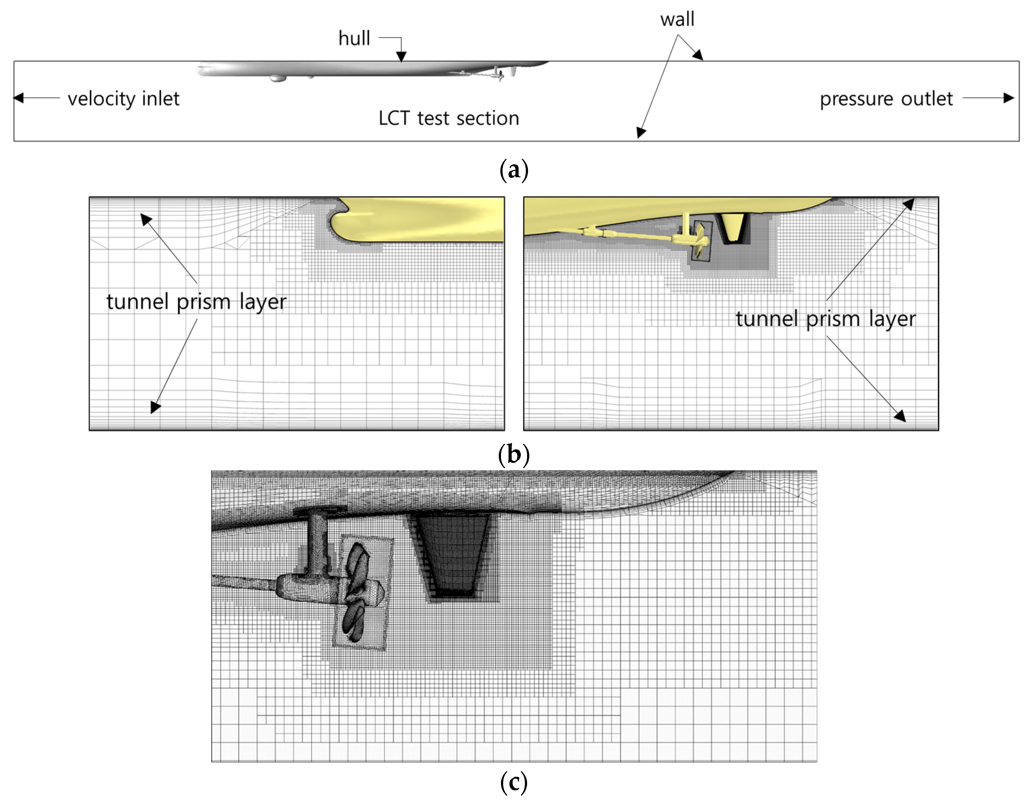
Figure 11 shows the computational domain reproducing the test section in LCT and boundary conditions (a), and the mesh distribution around the stern of the ship model (b, c). The velocity inlet and pressure outlet boundary conditions were set at the inlet and outlet surfaces of the computational domain, respectively. The main flow speed ($U_o$) was imposed on the velocity inlet boundary with a turbulence intensity of 1% and a turbulent viscosity ratio of 10. In addition, the gradient of the pressure was set to zero. The detailed expressions on the free stream values of the turbulence variables can be found in Shih and Liou [16] and also STAR-CCM+ [17]. At the pressure outlet boundary, the pressure was zero, while the normal gradients of the velocity and turbulence variables were set to be zero. The no-slip wall boundary condition with the high $y^{+}$ wall treatment (wall function) implemented in STAR-CCM+ [17] was applied to the hull and four surrounding walls of the LCT test section. At the wall boundaries, the turbulent kinetic energy k and the gradients of the flow variables were zero but the turbulence dissipation rate ε was not zero, instead this variable was modeled in the mesh element next to the walls as follows:

$$\epsilon =\frac{C_{\mu }^{\frac{3}{4}}{k}^{\frac{3}{2}}}{\kappa n_p}$$

(4)

where, $C_{\mu }$ is a model constant of 0.9, $\kappa$ is the von Karman constant ($\kappa$ = 0.41) and $n_p$ is the distance of the center of the first mesh element from the wall.

Figure 11b shows the prism mesh layers for capturing the boundary layer flows on the top and bottom surfaces of the LCT test section. The total mesh number in the numerical simulation was about 10 million (M), in which about 2M mesh elements were used in the propeller region.

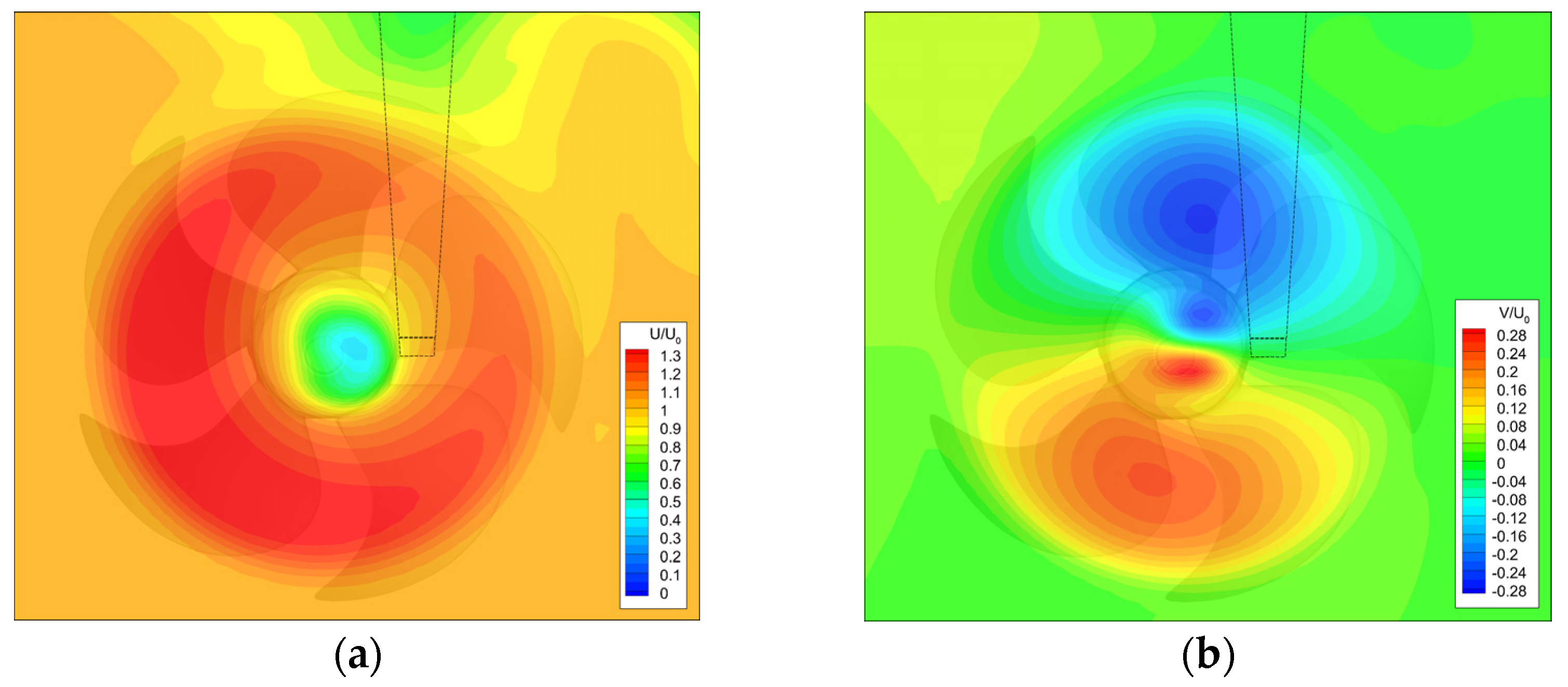
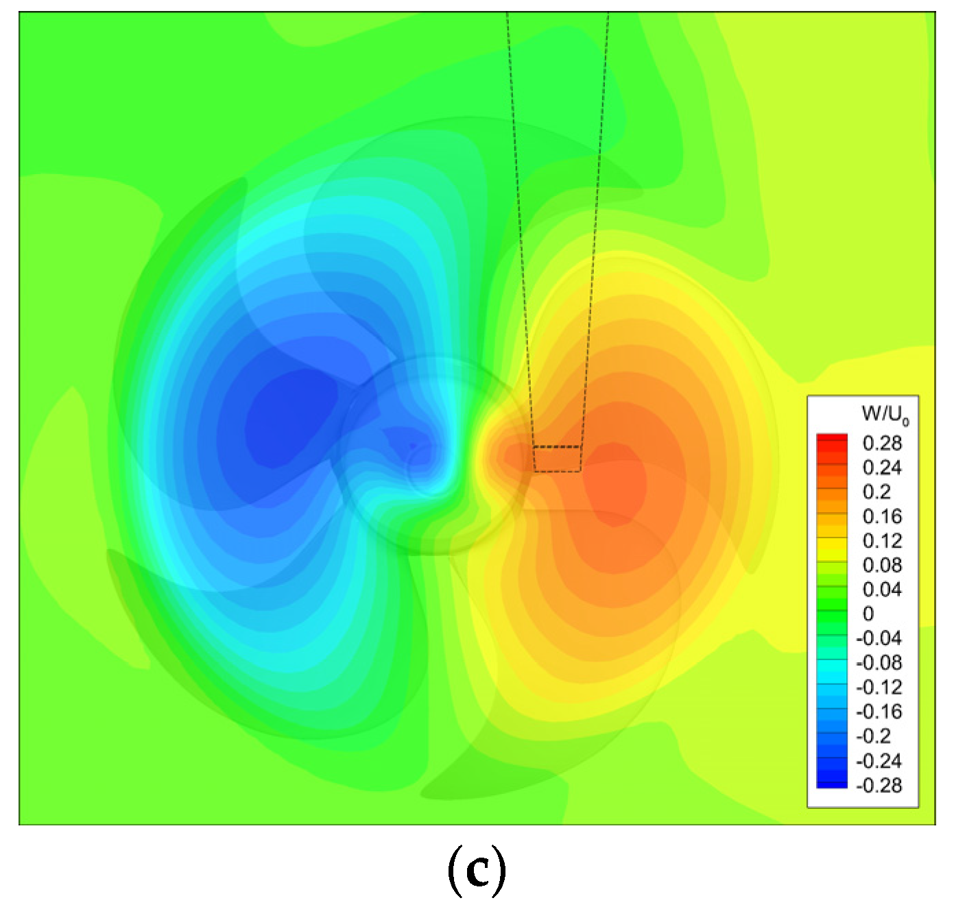
The rudder inflow calculated at the model speed ($U_o$) of 9 m/s and propeller rotation rate of 31 rps is shown in Figure 12, which was used to obtain rudder incidence angle. The detailed conditions for the current numerical analysis according to the model test conditions are provided in the next section. The time–mean velocity distribution shows the properties of rudder inflow well because the propeller rotates outward (counterclockwise rotation looking downstream at port (left) side). The accuracy of the current numerical results was validated with the measured velocity profiles and rudder inflow angles for different rudder angles, which can be found in the following section.

5. Measurements of Rudder Inflow and Observation of Rudder Cavitation

The rudder inflow between the propeller and the rudder was measured with the 3-D LDV system. The navy ship model has a 2300 ton class hull form and the principal particulars of it are expressed in

Table 3. Principal particulars of the model ship.

Length	7.07 m
Breadth	0.86 m
Draught	0.27 m
Max. ship speed	30.0 Kts

.

The ship model installed in the test section of the LCT is shown in Figure 13. The particulars of the full-spade rudder are also shown in

Table 4. Particulars of the rudder.

Rudder Type	Full-Spade
Balance ratio	0.226
Aspect ratio	1.5
Taper ratio	0.45
Section shape	NACA00XX
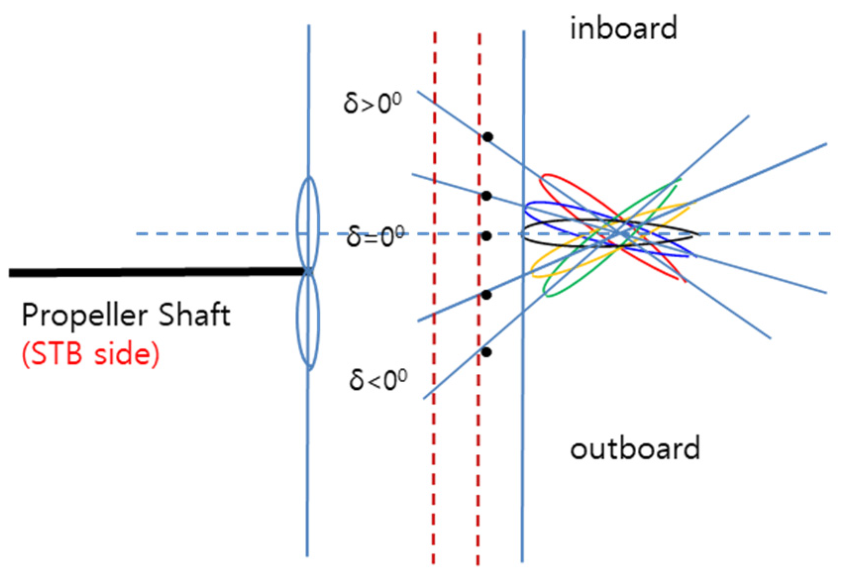
(bottom, tip)	NACA00XX

. The rudder part in contact with the stern hull of the ship model was referred to as the ‘bottom’, and the part located at the end of the span in the opposite direction of gravity was referred to as the ‘tip’. The description of the rudder deflection angle δ is shown in Figure 14.

In this study, 3-D LDV measurements were performed on the full-spade rudder models under the following test conditions.

-

Propeller: 1 type

-

Full-spade rudder: 2 types (flat-type, asymmetry-type)

-

Main flow speed U_o at the inlet of the test section: 9.0 m/s

-

Propeller revolution number per second (rps): 31

-

Propeller thrust coefficient (K_T): 0.1741

-

Static pressure in the test section: pressuring (non-cavity condition)

-

Rudder deflection angle: 0°~±16°

-

Reynolds number based on the ship length: 6.3 × 10⁷

-

Density of fresh water in the tunnel: 1000 kg/m³

The thrust coefficient K_T is defined as follows,

$$K_T=\frac{T}{\rho n^2{D}^4}$$

(5)

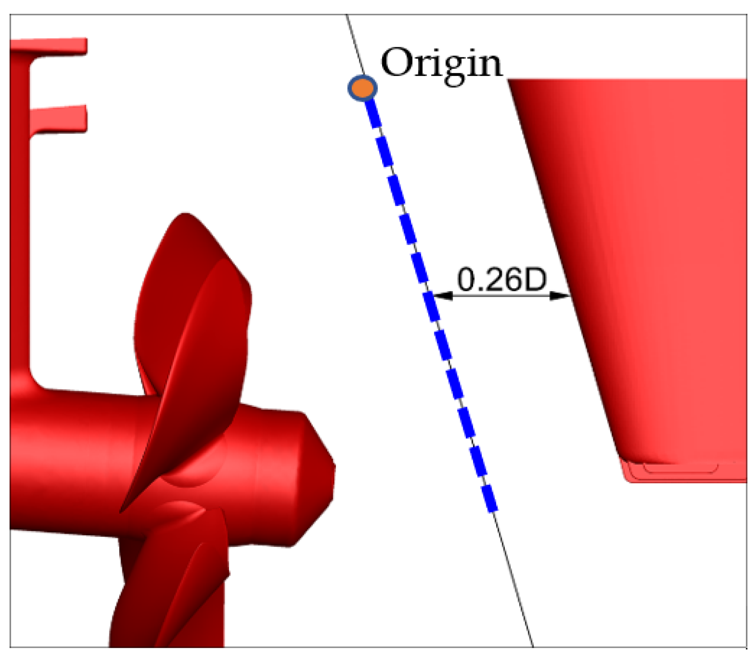
Here, T, $\rho$, n, and D are the propeller thrust, the density of fresh water, the propeller revolution number per second, and the propeller diameter, respectively. The inflow of the flat-type rudder under propeller operation was measured with the 3-D LDV system as in Figure 15. The measurement position of the 3-D LDV was set on the right (STB: starboard) side rudder and expressed in Figure 16. The LDV measurement position was set 0.26D apart from the rudder leading edge, where the rudder did not affect the flow in front of its leading edge in the slipstream. The origin is positioned at the same height as the rudder bottom.

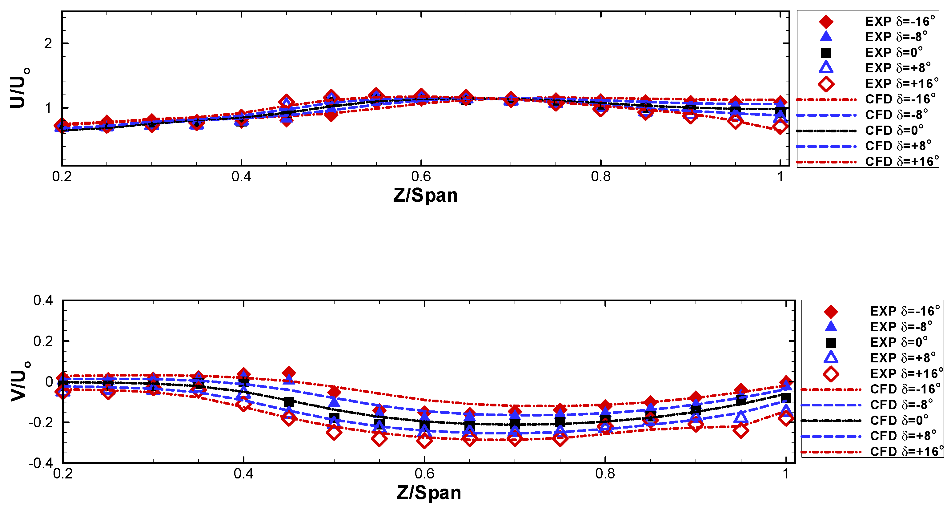
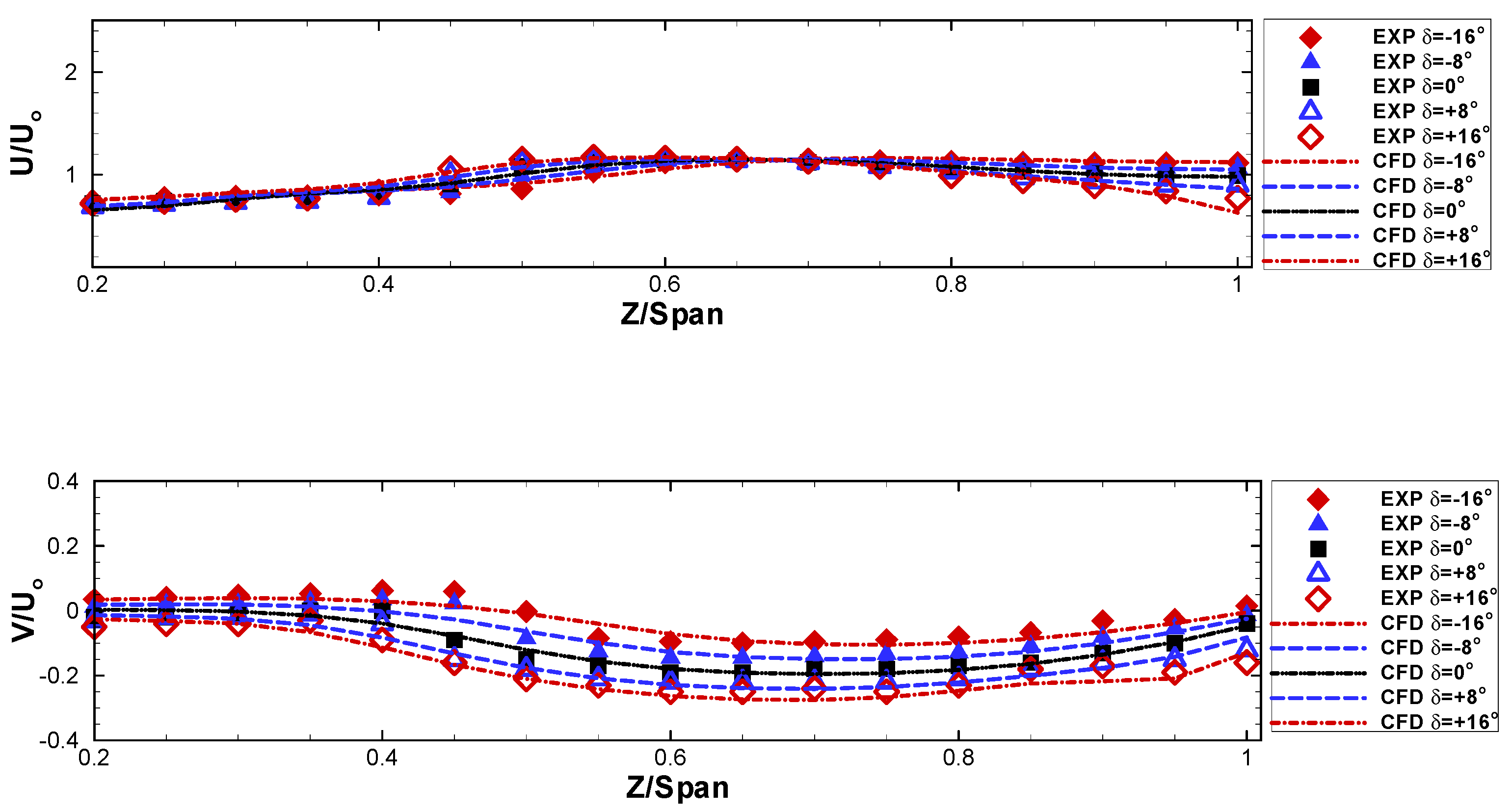
Figure 17 shows the comparison between experimental results (EXP) and numerical results (CFD). After defining the surface at a specific location over the rudder by LDV, the measurement grid for LDV and the grid for numerical simulation were matched well. The U velocity has a high magnitude in the range of 0.4 < Z/Span < 0.8 due to the high momentum in the propeller slipstream and an approximately 20% higher value near Z/Span = 0.6 than the freestream velocity, which is a well known flow characteristic in ship hydrodynamics. The V velocity also has a large magnitude at the range of 0.4 < Z/Span < 1.0 and a negative sign in the whole rudder span, which affects the sign of the rudder incidence angle.

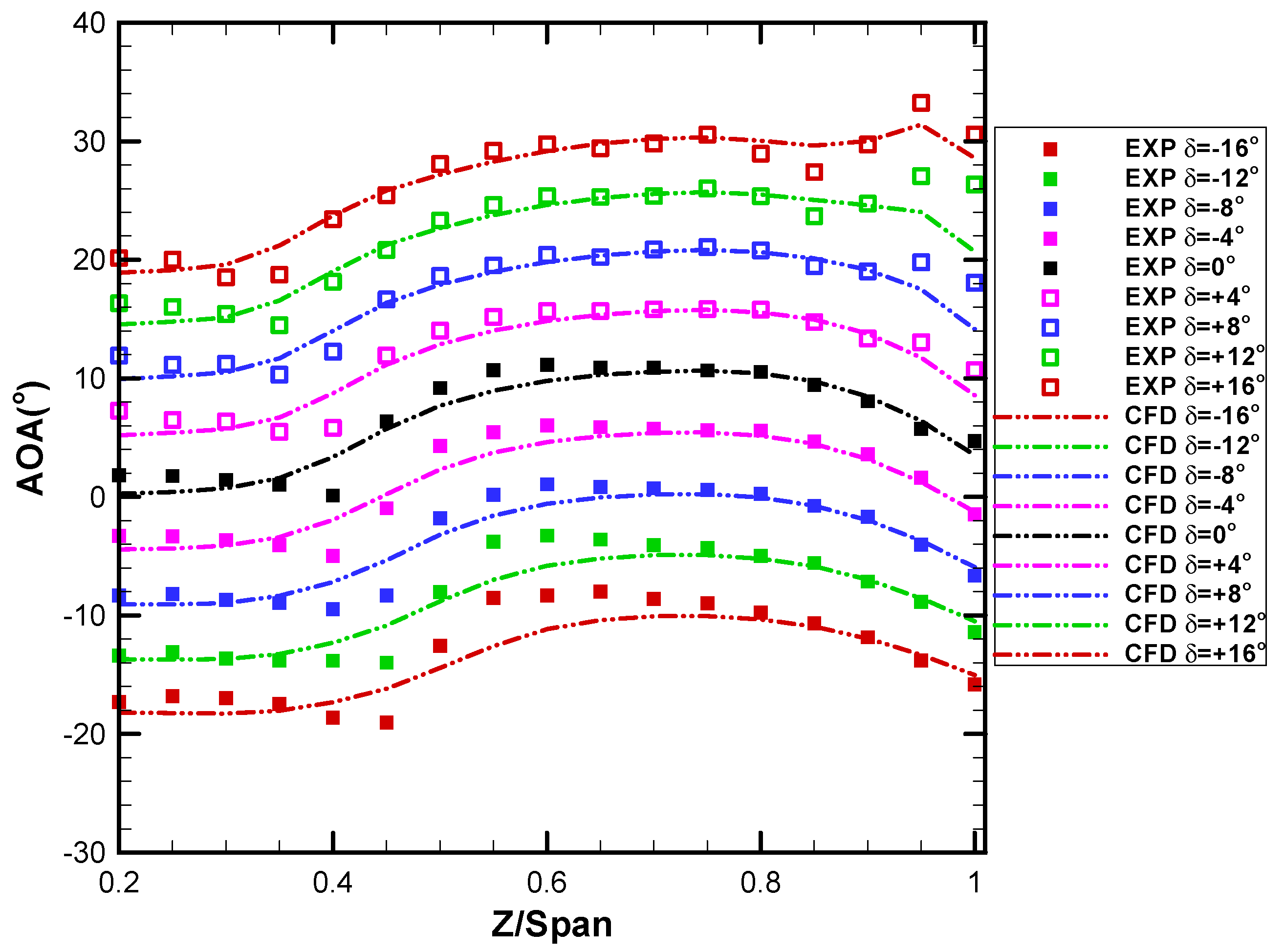
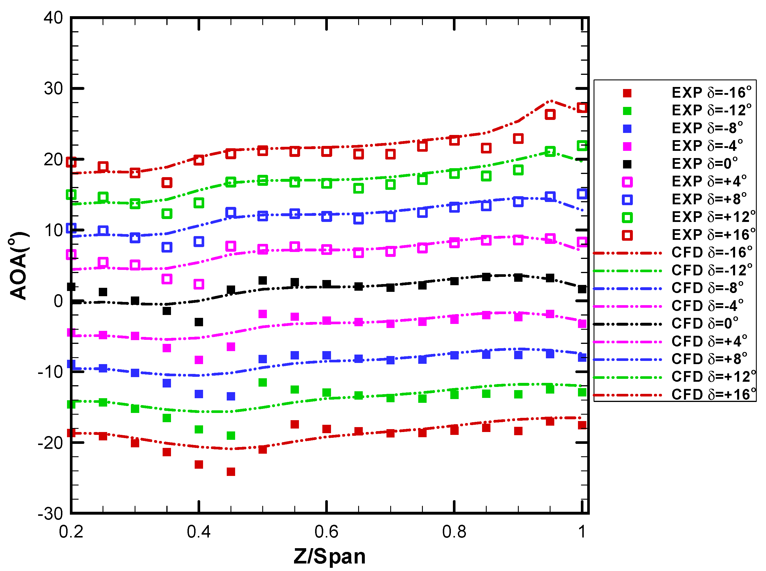
The incident angle (AOA: angle-of-attack) of rudder inflow was also extracted from the measured 3-D velocity components and described as in Figure 18. The comparison results of rudder incidence angle shows a little difference in the region of 0.2 < Z/Span < 0.4, however, those data from CFD and EXP were very similar at 0.4 < Z/Span < 1.0 (tip). The measured incident angle showed that it was not zero at the range of 0.4 < Z/span < 1.0 in the rudder deflection angle of 0° because of the propeller revolution and the swirl flow in the propeller wake. It can be seen that the magnitude of the AOA of the rudder inflow increases as the rudder deflection angle increases. Since the most critical thing in the AOA is the V velocity component, the comparison results in Figure 18 present that the 3-D LDV is a promising tool for measuring the rotational velocity components of rudder inflow efficiently.

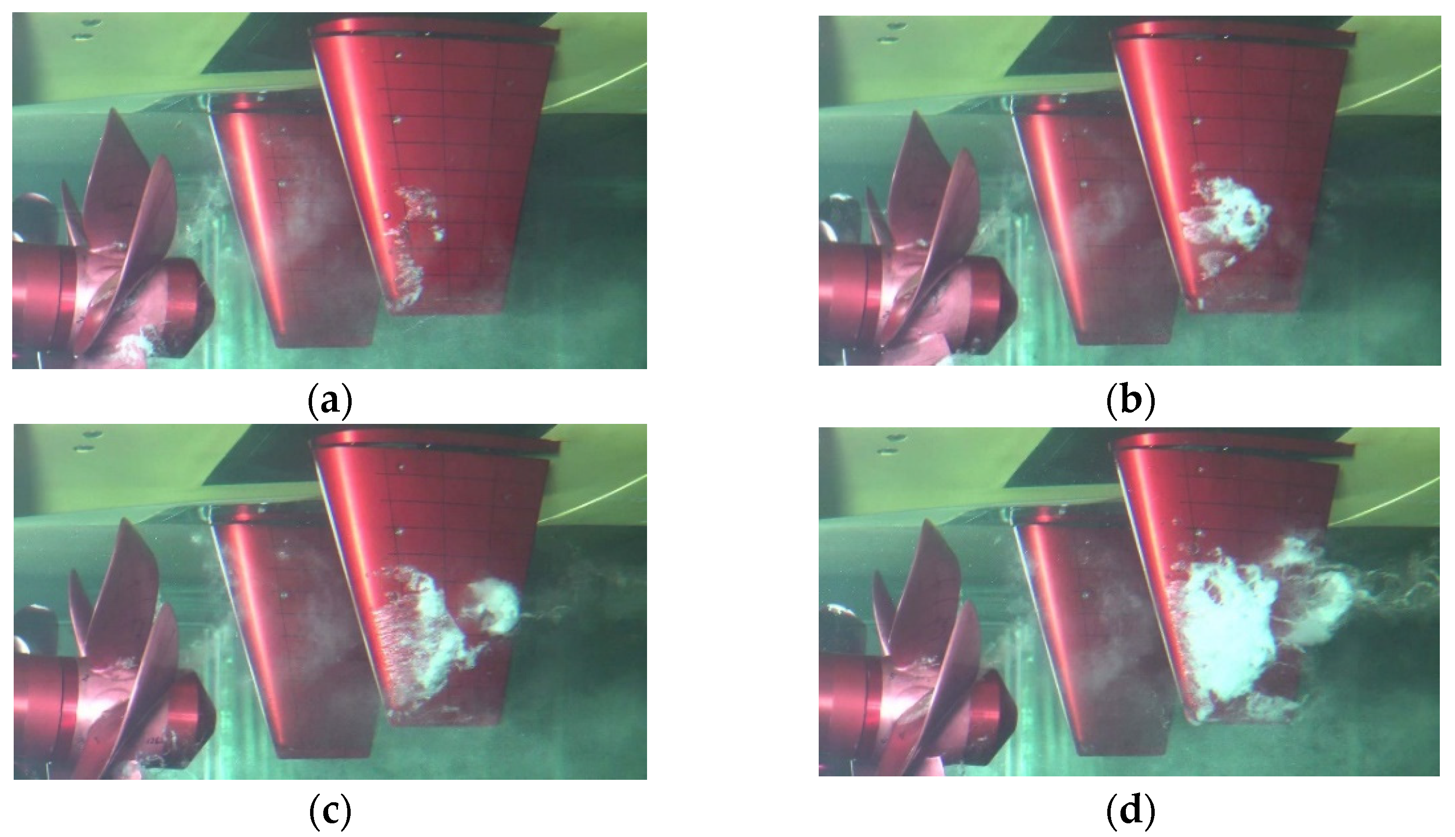
In addition, the rudder incident angle is closely related to rudder cavitation. Figure 19 shows the observation results of cavitation on the rudder model surface. The rudder cavitation tests were separately conducted at the condition of cavitation number ${\sigma }_V$ = 1.32 in the large cavitation tunnel, which was corresponding to the maximum speed of the ship.

-

Propeller: 1 type

-

Full-spade rudder: 2 types (flat-type, asymmetry-type)

-

Main flow speed U_o at the inlet of the test section: 9.0 m/s

-

Propeller revolution number per second (rps): 31.73

-

Propeller thrust coefficient (K_T): 0.1879

-

Rudder deflection angle: 0°~±16°

-

Reynolds number based on the ship length: 6.3 × 10⁷

-

Density of fresh water in the tunnel: 1000 kg/m³

The cavitation number is defined as follows:

$${\sigma }_V=\frac{P_0-P_v}{0.5\rho U_0^2}$$

(6)

where P₀ and P_v are the static pressure in the test section and the vapor pressure of fresh water, respectively. From the rudder deflection angle of 0° to −2°, the weak separation of the shear flow at the leading edge formed the sheet cavitation on the rudder surface. The sheet cavitation locally occurred at the region of 0.5 < Z/Span < 0.9 as shown in Figure 19a because the AOA distribution shows high values of 5° to 10° even at the rudder deflection angle of 0°. Since the rudder angle is maintained at around 0° when the ship travels straight, it is necessary to improve the rudder shape to reduce the cavitation occurring on the rudder surface, considering the AOA caused by the rudder inflow. As the rudder deflection angle increased more to −4° or −8°, the strong shear flow separation occurred and formed cloud cavitation with re-entrant flow beneath the cavity lump [18]. Figure 19 also shows that violent and large cavitation occurred at over −4°, and it can develop into cloud cavitation displaying a large amount of cavitation shedding and collapsing with the increase in rudder angle.

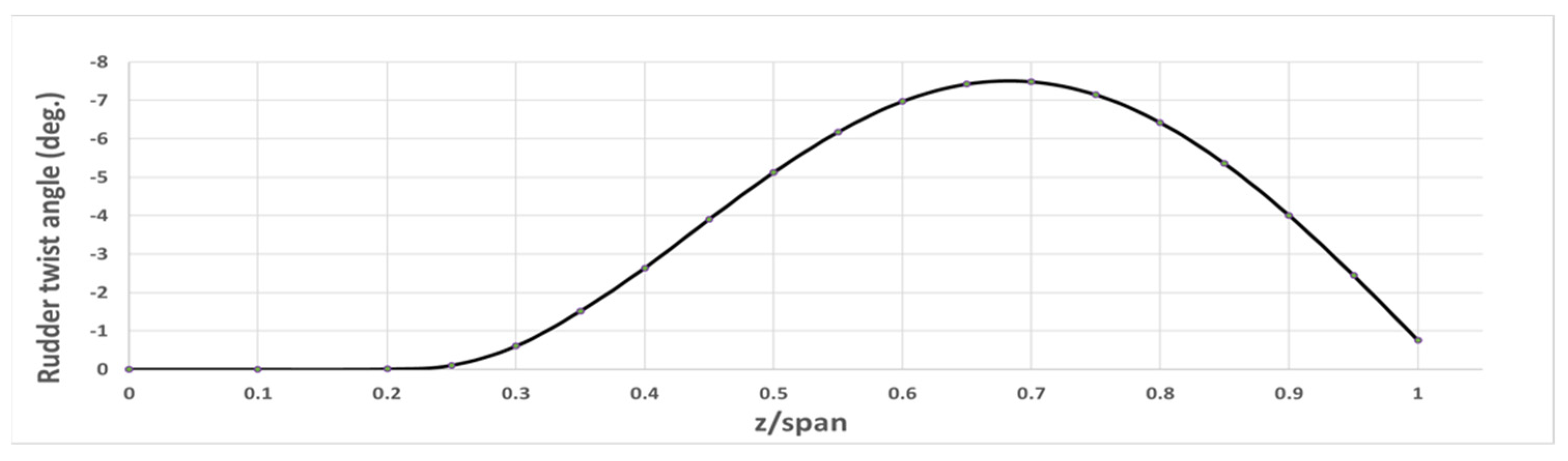
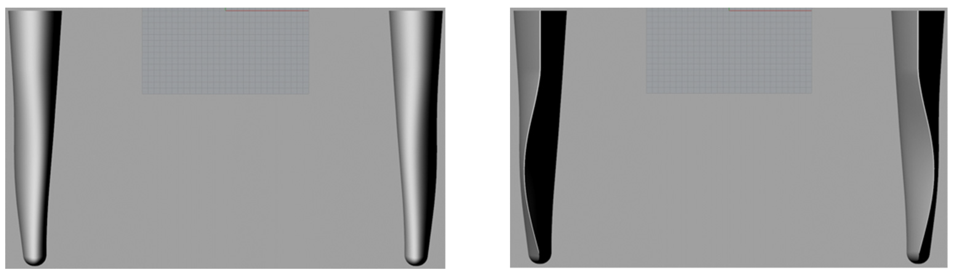
As the cavitation collapsing is known to be related to erosion on the rudder surface, the possibility of cavitation erosion may be significantly decreased if appropriate improvements on rudder shape are carried out based on rudder inflow information. Thus, in the present study, the asymmetry-type rudder was proposed in order to improve the cavitation performance of the flat-type rudder using inflow incidence angle. 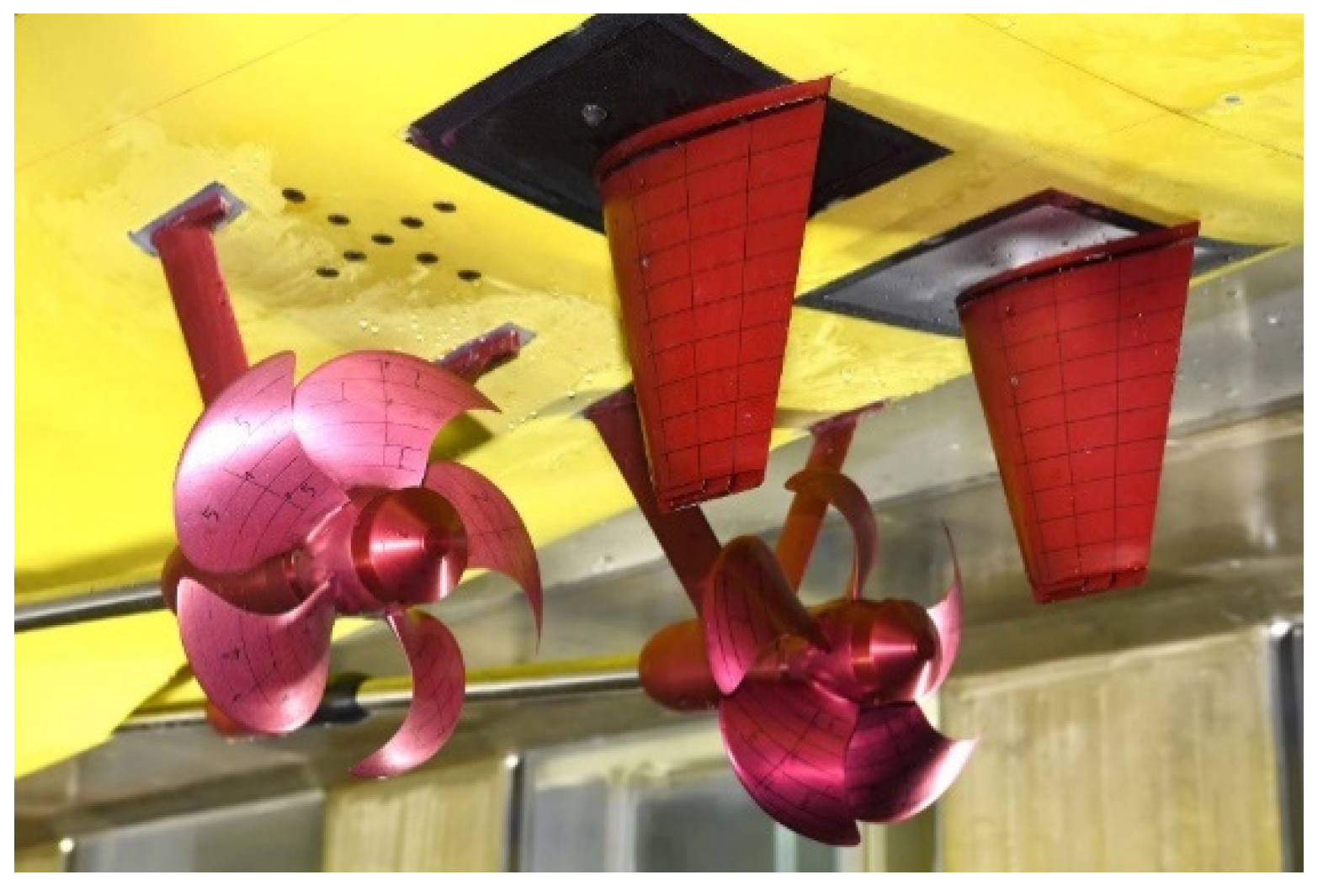The twist angle distribution for the asymmetry-type rudder was designed as in Figure 20 by using the flat-type rudder’s AOA measured by the 3-D LDV. Symmetric rudder sections were twisted around the rudder stock in a spanwise direction to produce the shape of the asymmetry-type rudder. The 3-D modeling for the fabrication of the asymmetry-type rudder is shown in Figure 21. The designed asymmetry-type rudder was produced and set in the test section of LCT as in Figure 22.

Figure 23 shows the comparison between experimental results (EXP) and numerical results (CFD) of velocity profiles of the asymmetry-type rudder inflow in the horizontal plane. The U velocity has high magnitude in the range of 0.4 < Z/Span < 1.0 due to high momentum in propeller slipstream, which is very similar to that of the flat-type rudder. The V velocity has a large magnitude at the range of 0.4 < Z/Span < 0.8, however, it shows a rather small velocity magnitude and causes a smaller rudder incidence angle than that of the flat-type rudder.

The AOA were also obtained and compared with the numerical simulation. As seen in Figure 24, the AOA is close to 0° and a constant value along the spanwise direction at the rudder deflection angle of 0°. There is little difference between measurements and CFD at the range of 0.2 < Z/Span < 0.4, however, the numerical simulation is found to be well matched with experimental results at the other range. It is interesting to note that the AOA hump in the range of 0.4 < Z/Span < 1.0 as seen in Figure 18 disappeared in the asymmetry-type rudder, and it showed nearly constant AOA distribution at each rudder deflection angle as in Figure 24. Originally, we designed the rudder incidence angle to be 0° by the contribution of a twisted angle distribution, however, it showed some difference of about 1°~3° at all spanwise positions at the rudder deflection angle of 0°. To investigate the effect of this incidence angle difference on rudder cavitation, the rudder cavitation observation was additionally conducted for the asymmetry-type rudder. The experimental conditions were the same as those of the flat-type rudder.

Figure 25 shows the cavitation observation results of the asymmetry-type rudder at four rudder defection angles. There is no cavitation on the rudder surface at the rudder deflection angle of 0° and small amount of cavitation occurred at the rudder angle of −2° and −4°. In the case of the flat-type rudder, a large amount of cavitation appeared even at the rudder angles from 0° to −4° as in Figure 19.

It can be also seen that the amount of cavitation is significantly reduced in the asymmetry-type rudder even at the rudder angle of −8°, compared with that in the flat-type rudder. A ship is generally sailing straight in the state of the rudder deflection angle of 0°~±4° on a cruise route, and thus the minimization of the cavitation amount at those small rudder angles is very important in the viewpoint of rudder cavitation performance. In this context, the asymmetry-type rudder based on the rudder incidence angle will be highly effective against rudder cavitation erosion on its surface and cavitation noise.

6. Conclusions

The rudder inflow formed behind a propeller attached to a ship model was investigated by the 3-D LDV system in a large cavitation tunnel. The beam probes of the 3-D LDV system were not emerged in the tunnel water but placed outside the tunnel’s test section. To obtain the reliability of the transverse velocity component in flow measurements, the calibration procedure with the help of water injection device was additionally introduced and found to be working well.

The three-dimensional velocity components of the rudder inflow were coincidently measured by the 3-D LDV system placed outside the test section, which was conducted in the large cavitation tunnel for the first time in the world. The measured data were compared with those obtained by numerical simulation. The full appended ship model installed in the cavitation tunnel was considered in mesh generation, and the propeller flow was directly solved using the sliding mesh method in the numerical calculation. The experimental and numerical results showed very similar velocity profiles in the rudder inflow in streamwise- and transverse-direction. From the velocity components in the rudder inflow, the rudder incidence angle was extracted and showed high values at 0.4 < Z/Span < 1.0 where the cavitation mainly appeared by large hydrodynamic loading on the rudder surface. Through these results, it is found that the 3-D LDV system could provide an effective tool for measuring three-dimensional velocity components between the rudder and the propeller, even in a large cavitation tunnel. In addition, reliable measurements of the rudder inflow using 3-D LDV system would be helpful for improving the rudder design, which aims to reduce the rudder erosion by violent cavitation on its surface since the rudder incident angle is closely related to rudder cavitation. In the present study, the asymmetry-type rudder was designed based on the rudder incidence angle distribution of the flat-type rudder, and the rudder cavitation performance in the asymmetry-type rudder was found to be significantly improved compared with the flat-type rudder through cavitation model tests.