Article

Wave Energy Dissipation of Spilling and Plunging Breaking Waves in Spectral Models

1
Shirshov Institute of Oceanology, Russian Academy of Sciences, Nahimovskiy Prospekt, 36, 117997 Moscow, Russia
2
Department of Civil Engineering, Gebze Technical University, Gebze 41400, Turkey
3
Department of Civil Engineering, Yildiz Technical University, Esenler, Istanbul 34220, Turkey
*
Author to whom correspondence should be addressed.
J. Mar. Sci. Eng. 2022, 10(2), 200; https://doi.org/10.3390/jmse10020200
Submission received: 2 January 2022 / Revised: 23 January 2022 / Accepted: 29 January 2022 / Published: 1 February 2022
(This article belongs to the Special Issue Nonlinear Wave Dynamics and Wake Structure)

Abstract

:
On the basis of field experiments and modeling, the dependence of the dissipation of the energy of waves breaking by plunging and spilling on the frequency of wave spectra was investigated. It was shown that the modeling of wave breaking should take into account the compensation of the nonlinear growth of higher wave harmonics, which occurs in different ways for waves breaking with different types and for different methods of modeling a nonlinear source term. The study revealed that spilling breaking waves have a frequency selectivity of energy dissipation at frequencies of second and third harmonics for the Boussinesq and SWAN models for any method of modeling a nonlinear source term. Plunging breaking waves have a quadratic dependence of the dissipation coefficient on frequency in the Boussinesq model and SWAN model with the SPB approximation for a nonlinear source term. The SWAN model with default LTA approximation for plunging breaking waves also assumes frequency-selective energy dissipation. The discrepancy between the LTA default method and others can be explained by the overestimation of the contribution of the second nonlinear harmonic and by inaccurate approximation for the biphase. It is possible to improve the accuracy of LTA and SPB methods by tuning SWAN model coefficients.

1. Introduction

Almost all modeling of the dynamic processes occurring in the coastal zone of the sea begin with estimates of the wave parameters. When approaching the shore and with decreasing water depth, the waves transform, becoming steeper and more asymmetrical, and then breaking. The process of wave breaking is characterized by significant losses of their energy. Changes in the steepness of waves and their asymmetry, occurring both due to linear and nonlinear processes and due to breaking, lead to a change in the higher statistical moments of wave motion, which determine the magnitude and the direction of sediment flow in the coastal zone [1].
There are a number of models that describe, with high accuracy, the linear and nonlinear transformation of waves over the real bottom topography in the coastal zone. However, dissipation processes have been much less studied. There is no generally accepted and well-tested model of wave energy dissipation in the surf zone or an accurate physical description of changes in wave properties during the dissipation process [2]. In general wave models can be divided in to phase resolving and phase averaged. The first usually are solved using hydrodynamic equations in the time domain, and the second represent the wave spectrum evolution in the frequency domain based on the wave action balance equation (for example, SWAN (Simulating WAves Nearshore) model). Some phase resolving wave models are solved by spectral methods in the frequency domain that are less time-consuming in modeling as compared to the time domain simulation. Spectral method modeling results in the complex amplitudes of wave harmonics (deterministic models [3,4,5]) or the modulus of complex amplitudes and biphases (stochastic models [6]). Together with the modeling of the spectrum itself, phase-resolving models allow using the inverse Fourier transform to determine the free surface elevations and the velocity field.
The main difficulty in accurate representation and modeling wave breaking in phase-resolving models is to account for the spatio-temporal occurrence of breaking events in combination with the type of wave breaking. Recent investigations confirm that models can reproduce the overall behavior of wave breaking dissipation, but this does not necessarily mean that the process itself is modeled with physically accuracy [7]. In spectral-type models, the main challenge is to describe the effect of wave energy dissipation due to breaking on the frequency structure of waves and wave spectrum shape [4].
To assess the effect of wave breaking on the amplitudes of wave harmonics and wave spectrum shape, two approaches are now used:
(1) the wave breaking does not change the shape of the spectrum, but only reduces the spectral density of waves by the same factor for all frequencies, so-called independent wave energy dissipation [8,9,10];
(2) the spectral density during wave breaking decreases, depending on the square of the frequency [4,11].
The use of the uniform wave energy dissipation coefficient for modeling in spectral phase-resolving models showed a fairly good agreement between the model and experimental results [10,12]. The concept of uniform or frequency-independent (or uniform) energy dissipation is often used in modeling the evolution of spectra in phase-averaged models, for example, SWAN. Spectral shapes in shallow water areas are modified by triad wave interaction equations in phase-averaged spectral wave models.
The combination of the two approaches offers an empirical formula that assumes a partial dependence of the dissipation coefficient on the square of the frequency: during wave breaking in one frequency range of the first and lowest harmonics the energy decreases uniformly, but in the high-frequency range it has quadratic dependence on the frequency [4,13]. The quadratic type of the dependence was shown theoretically using the equations of the eddy viscosity model [11]. There are some other frequency dependencies of energy dissipation; for example, the dependence on the fourth power of frequency was demonstrated in [14].
By comparing laboratory experimental data and modeling, it was found that in the case of using a finite-difference model of eddy viscosity for modeling breaking waves, the dependence of the rate of dissipation of wave energy on frequency is inversely proportional to the spectral density for waves with a random phase. However, this dependence does not hold for wave groups. It was noted that, apparently, wave groups on the whole are subject to dissipation to a greater extent than waves, equivalent in spectral parameters without a group structure [15].
Based on the data of two field experiments, it was shown that in the outer part of the surf zone, the dissipation of wave energy is practically independent of frequency, and in the inner part of the surf zone, there is either a partially quadratic or selective (at frequencies of the second and third harmonics) dependence of the wave energy dissipation on frequency. It was noted that the type of frequency dependence of the dissipation of wave energy inside the surf zone is determined by the wave asymmetry and the bottom slope [16]. Increased values of energy dissipation at frequencies of the second and third harmonics were also obtained in laboratory experiments described in [17].
Comparison of the simulation results with the data of laboratory and field experiments [12] showed that the exact form of the frequency dependence of energy dissipation is not so important for calculating and modeling wave spectra. However, by comparing the simulation results with experimental data, it was shown that the exact form of the frequency dependence of energy dissipation has a significant effect on the values of the higher wave statistical moments obtained from the elevations of the free surface, which is of great importance for assessing the processes of sediment transport (for example, [14,18]).
Analysis of waves breaking in the surf zone showed that the energy losses observed in the wave spectrum are primarily the result of nonlinear transfer from the spectral peak to higher frequencies, and therefore energy dissipation occurs mainly in the high-frequency part of the spectrum [19]. This indicates that nonlinear processes can play a more significant role in the transformation of the wave spectrum than processes caused by collapse. As studies of recent years have shown, nonlinear processes of wave transformation largely determine the processes of breaking. For example, the different frequency composition of breaking waves (amplitudes of higher harmonics and the phase shift between them) leads to the breaking of waves of different types, which is determined by the conditions of wave transformation, for example, the conditions of “shallowness” of water [20]. It was shown that the breaking index, which relates the height of the breaking waves to the depth of breaking, depends on the nonlinear processes of wave transformation before breaking, and new formulas have been proposed for its determination [21,22]. However, how different formulas for the breaking index affect the frequency dependence of the dissipation of wave energy during breaking has been insufficiently studied, which is still relevant both for physical processes and for model applications.
When studying the change in the shape of the spectrum of breaking waves by comparing the field data of two experiments and the data of numerical modeling without taking into account dissipation, it was revealed that the breaking compensates the processes of linear and nonlinear transformation of waves “fitting” the spectrum to a universal form [16].
This means that the dissipative term depends partly on the nonlinear term, how it is modeled, and what the accuracy is. Recently, according to the data of field and laboratory experiments, it was shown that waves breaking by different types have different nonlinear properties and spectral composition, namely, a different ratio between the amplitudes of the first and second harmonics and the phase shift between them [20,22]. This suggests that with the same method of simulating nonlinearity, the dissipative term can have a different structure for waves breaking with different types.
Thus, it can be stated that, when describing dissipation processes, there is no unified approach and universal dependence for energy dissipation during wave breaking on frequency or a clear physical description of changes in wave spectrum during their breaking under the influence of dissipative and nonlinear processes. Meanwhile, modeling is now the main method for studying the dynamics of the coastal zone. When simulating the process of breaking waves, it is important to understand how accurately the processes are simulated and how applicable the parameters are of the models offered by default.
The main purpose of this work is to study the necessary dissipation term and the dependence of the dissipation of the spectral energy of waves breaking by different types on the spectral frequency at the modeling wave spectrum by phase-resolving and phase-averaged models, with recommendations on default nonlinear terms. The problem will be solved based on the comparison of data of a field experiment and on numerical simulations for more frequently used models.

2. Methods

2.1. Field Experiment

The experiment “Shkorpilovtsy-2007” was carried out on the Black Sea in September–October 2007 on the pier of the Institute of Oceanology of the Bulgarian Academy of Sciences. The length of the pier, specially designed for coastal zone dynamics research, is 230 m. The pier has a single line of rare piles, minimizing the influence on the wave field measurements. The pier is located in the middle of an almost straight-line section of the coastline of sandy beach. During the experiment, 8 capacitive wire string wave gauges (sampling frequency 200 Hz) and 7 resistance wire wave gauges (sampling frequency 5 Hz) were installed. The typical synchronously measured on the 15 gauges of wave chronograms registered on 27 September 2007 was selected for analysis. The duration of the selected wave records was 20 min. On this day, the wave regime changed very little. It was not a windy day, and swell waves broke in two types. At a distance of 160–170 m, the wave break was the spilling type, and closer to the shore, the plunging type (at a distance of 60–70 m). The scheme of the experiment and positions of wave breaking are shown in Figure 1. A more detailed description of the wave regime on that day is given in [1,20,23,24]. For the analysis, we selected chronograms of wave transformation between gauges 9 and 12 (spilling breaking) and 1 and 4 (plunging breaking). The wave spectra at the points before and after wave breaking are shown in Figure 2.

2.2. Wave Energy Dissipation Coefficient

In nature, nonlinear and dissipative wave transformation processes occur simultaneously. The only way to separate them is to use modeling with alternate an artificial switching of on and off of different model blocks or terms of equations responsible for modeling the processes of interest to the study. This technique is often used, for example, when investigating the movement of ships in complex nonlinear wave conditions [25,26]. In order to estimate what the dissipative term should be, we simulated the propagation of waves from the beginning of the breaking to the moment of its end, with the dissipative term turned off, and compared the result with that measured in the field experiment. Thus, we were able to estimate the disparity necessary in order to compensate for the nonlinear changes that arose.
As was proposed in [11], the estimation of the dissipation coefficient (αn) as a function of frequency can be done on the basis of a comparison of the model wave spectra (without modeling wave dissipation, only wave nonlinearity is taken in account) and experimental wave spectra (naturally taking into account both wave nonlinear processes and dissipation):
α n = S ( x s t a r t + Δ x ) c a l c S ( x s t a r t + Δ x ) m e a s S ( x s t a r t ) m e a s ( 2 Δ x )
where S is the wave spectrum at the corresponding points, with the indices “calc” and “meas” marking the spectra calculated by the model without taking into account dissipation and the experimentally measured spectra, respectively; Δx is the distance of wave propagation; xstart is the coordinate of the starting point at which the modeling begin.
With such an estimate, it is assumed that dissipation does not affect the process of nonlinear deformation at a distance Δx, although, in fact, the rate of generation of new harmonics depends on the amplitudes of interacting harmonics, which can decrease along all considered distances due to dissipation during wave breaking. Thus, in the method used, the energy dissipation of breaking waves does not occur uniformly and constantly, but only once at the end of the considered distance, which does not correspond to the physics of the real continuous process of breaking waves and can lead to an underestimated dissipation coefficient. Detailed analysis of the possibility of using such an approach for qualitative assessments of the dependence of the dissipation coefficient on frequency is shown in [16].
The modeling was carried out using two spectral models: a phase-averaged SWAN model version 41.31AB [27,28] and a phase-resolving model based on Boussinesq-type equations, with improved dispersion characteristics solved by spectral methods [5].
In the frequency domain, Boussinesq equations represent a set of evolution equations for complex Fourier amplitudes (Ap), total number of complex amplitudes, and upper limit p, depending on the frequency discretization step.
d A p d x = β 2 h x h A p i 2 g ( F p + + F p ) α   n A p
where first term on the right side of Equation (2) describes the linear increase of amplitudes, hx is slope steepness, h is water depth, g is the gravitational acceleration, and αnAp is the dissipation term. As previously stated, our simulation was carried out without taking into account the dissipation, so the dissipation term was absent.
The second and third terms are, respectively, the summary and different triad interaction of harmonics, described by
F p = m = 1 α β 1 A m * A p + m exp [ i ( ψ m + p + ψ m + ψ p ) ]
F p + = m = 1 p 1 α + 2 β 1 A m A p m exp [ i ( ψ m + ψ p m + ψ p ) ]
where β1, α+, and α are interaction coefficients that depend on local depth (h), wave number (kp), and angular frequency (ωp). To save space, we do not show the formulas for β1, α+, α, and αn. They can be found in [5,11]. ψp is the phase, derived from
d ψ p d x = k p
The evolution equations for wave amplitudes in the frequency domain were solved numerically by the fourth-order Runge–Kutta method [5].
We chose this model among all other phase-resolving ones because, only for it, a spectral method solution was proposed in the frequency domain, in which there is also a model for the wave spectrum. This solution immediately gives the spectrum in the form of Fourier amplitudes. In this case, no additional procedures for constructing the wave spectrum are required, and it is easy to compare the solutions of two spectral models. Moreover this model in the frequency domain is analogous to MIKE 1D in the time domain. Its appreciability and accuracy have been investigated, for example, in [5,10].
For the phase-resolving Boussinesq-type model, the initial complex amplitudes of all harmonics were determined from the Fourier series expansions of the measured free surface elevations. Frequency resolution was 0.01 Hz, frequency range (0.01, 1.5) Hz. The wave spectra were calculated as the moving averaged squared modulus of complex amplitudes.
SWAN is a spectral modeling tool based on the solution of the wave action balance equation [29,30].
N t + C g , x N x + C g , y N y + C σ N σ + C θ N θ = S i n + S n l 3 + S n l 4 + S w + S s w   + S b + S b r σ
where N is the action density, t is the time, σ is the radian frequency, and θ is the propagation direction. N is the function of the space parameters (x, y), σ, and θ. Cg,x, Cg,y, Cθ, and Cσ are the group velocities in geographical and spectral spaces. S represents the sources or sinks of the wave energy, including the wind wave growth (Sin), nonlinear transfer of wave energy through three-wave (Snl3) and four-wave (Snl4) interactions, wave decay due to white capping (Sw), nonbreaking wave dissipation (Ssw), bottom friction (Sb), and depth-induced wave breaking (Sbr). Further details of the scientific background of the SWAN spectral wave model can be found in [27,28].
For the SWAN model at the input, the spectra constructed from the wave chronogram were set. The SWAN model was run on 1D stationary mode, with a horizontal discretization of 2 m, and in the spectral domain, the total number of frequencies was set as 38, with minimum and maximum frequencies of 0.04 and 1.4961 Hz. In the stationary mode, SWAN determines the initial guess conditions based on the 2nd generation source terms introduced by [31]. Dissipation terms were disabled, including breaking, white capping, turbulence, and bottom friction. No wind was considered during simulations due to field experiment conditions.
The nonlinear transformation of the spectrum was simulated in two different ways. The default nonlinear triad source term in SWAN is the Lumped Triad Approximation model—LTA [32,33]. This parametrization is based on the extended Boussinesq model suggested in [5]. The LTA uses a parameterization for the local bispectrum based on the local depth and the spectrum itself. The parameterization for the biphase of the self–self interactions is a function of the Ursell number [32,34]. The LTA considers only collinear self–self interactions for computational efficiency. It can result in a poor representation of the spectral shape and related integral quantities of, e.g., mean wave period. The inability of the LTA model to reproduce the transitions to the universal high frequency tail of the spectrum in shallow water was also shown, which is demonstrated in a number of previous observations [33].
The other possibility for the nonlinear triad source term in SWAN is the Stochastic Parametric model based on Boussinesq equations (SPB; [35]), which relaxes the constraint of only considering the self–self interactions and considers all interacting frequency components. This parametrization takes into account the wavenumber mismatch occurring in intermediate and shallow water depth. The SPB model provides better agreement with the observations. All higher harmonics are predicted relatively well, including the surf zone [21,36].
Evaluation of the dissipation coefficient according to Equation (1) was carried out between gauges 11 and 9 for spilling and between 4 and 1 for plunging breaking waves (Figure 1). The initial spectra were set from the experimentally measured free surface elevations on gauges 11 and 4.

3. Discussion of Results

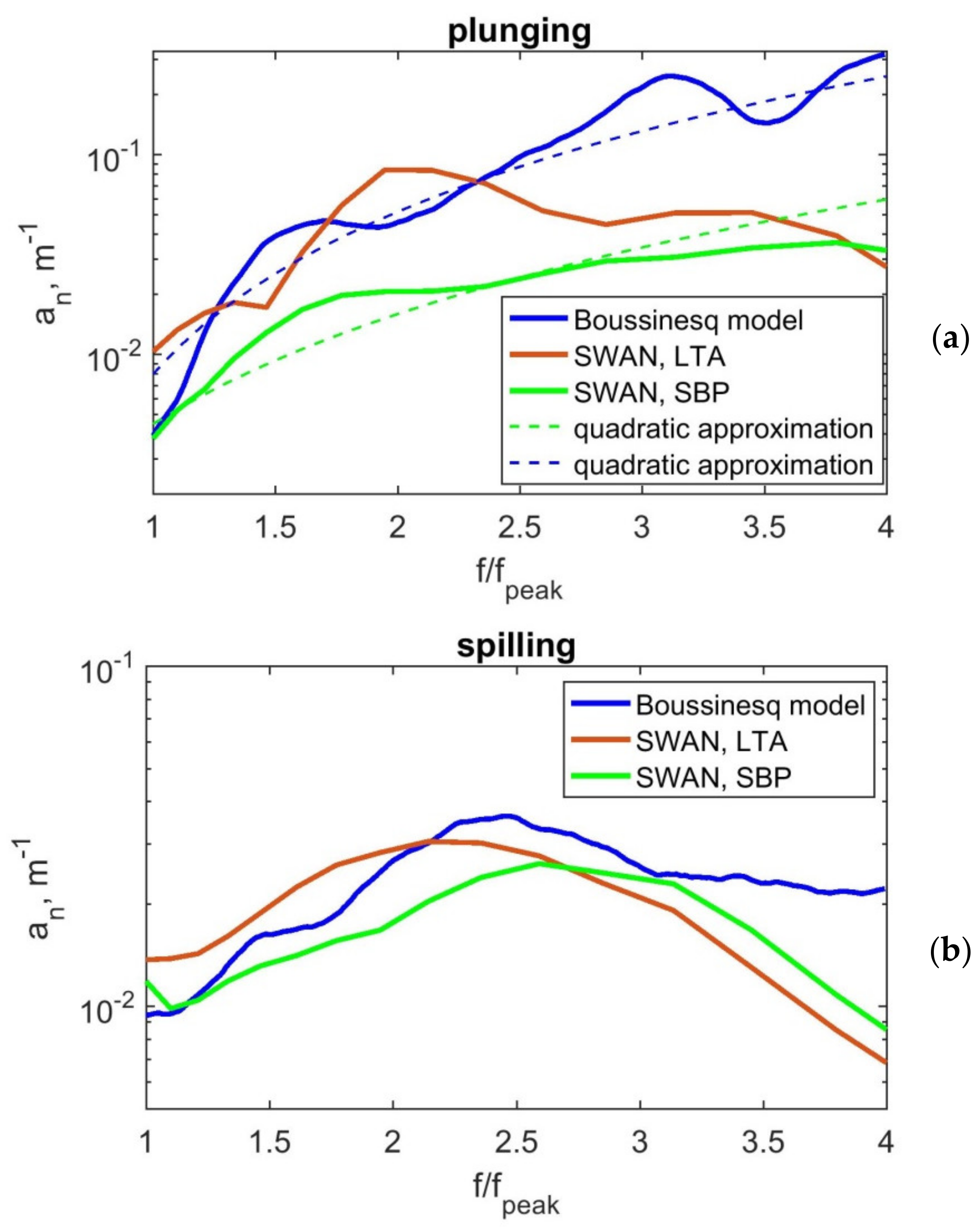
The dissipation coefficient (Equation (1)) calculated for different wave breaking types on the basis of the above-described models is shown in Figure 3. The frequency dependences of the dissipation coefficient presented in this figure differ but can be qualitatively classified as quadratic and selective. It can be seen that the form of the dissipation coefficient for spilling waves on a qualitative level is in agreement (Figure 3b). There is some selectivity of dissipation at frequencies of the 2nd and 3rd harmonics. However, since the coefficient itself has small values (in the order of 10−2), it can be assumed that the dissipation of all harmonics occurs approximately uniformly. As was mentioned in the introduction, this approach is implemented in many wave models. When comparing the dissipation coefficients for spilling and plunging waves, it can be seen that they are different in both models (Figure 3). Plunging waves dissipate more strongly and have a large dissipation coefficient, especially for higher harmonics. If we consider plunging breaking waves, in general we can say that dissipation occurs approximately according to the quadratic law when using Boussinesq and SPB modeling methods. This is the second way for the modeling of breaking waves suggested in [4]. For the SPB method, the quadratic dependence is small, while for the Boussinesq model it is significant. The LTA method still gives a frequency-selective dependence of the dissipation coefficient on the frequency of the 2nd harmonic. Taking into account the fact that for SPB the dependence of the dissipation coefficient on the square of the frequency is small, it can also be considered approximately constant (uniform dissipation).
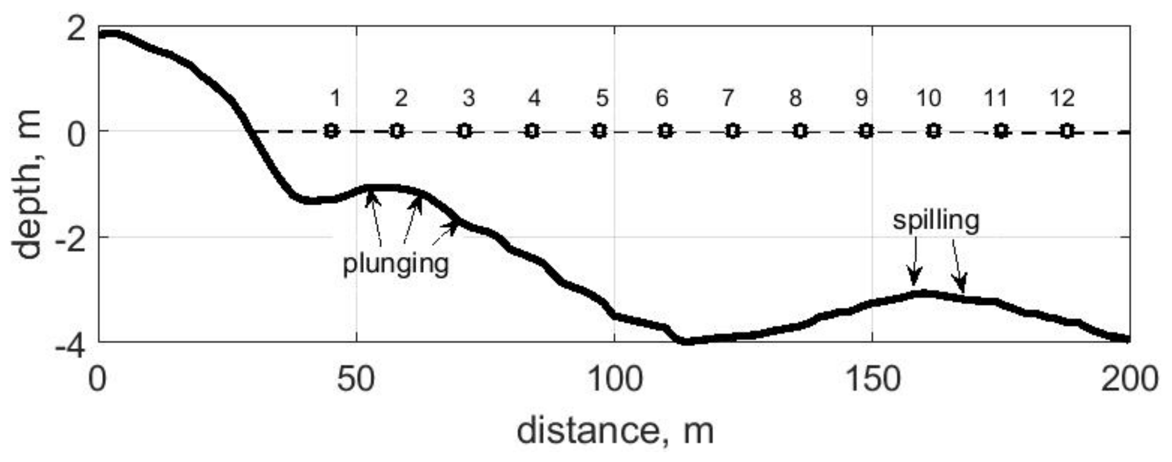
Let us consider the contribution of linear and nonlinear wave transformation processes to wave spectrum shape of differently breaking waves. Note that plunging and spilling breaking waves transform and break over different bottom slopes. We simulate the propagation of waves with the “switching off” of the model terms responsible for (a) the nonlinear triad interactions and (b) the linear transformation of waves. As was mentioned above, in real conditions, linear and nonlinear transformations of waves occur together, and it is impossible to strictly carry out such an artificial separation; however, in modeling, the intensity of manifestation of certain processes in the wave spectra, depending on the conditions of their transformation, can be demonstrated quite clearly.
Figure 4 and 
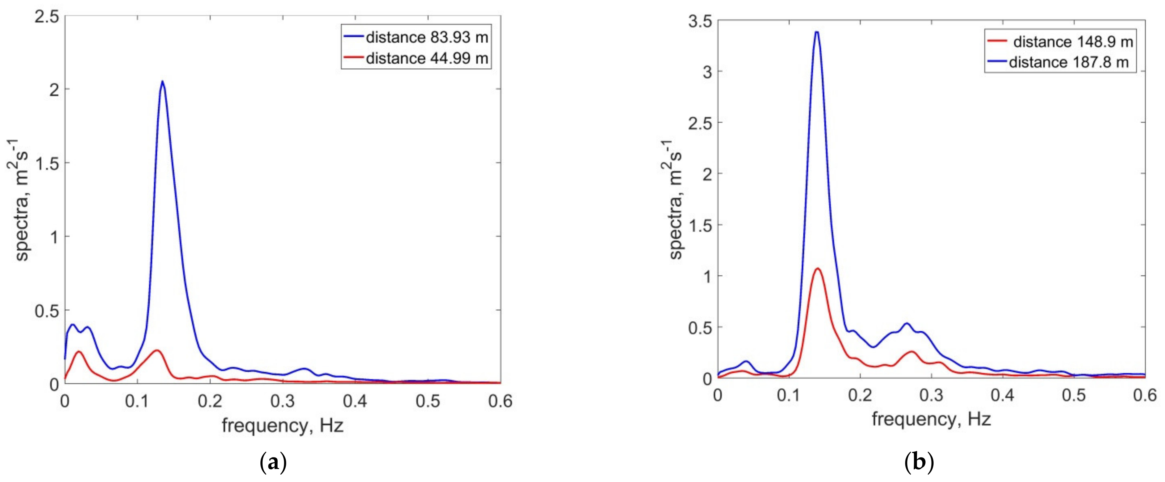
Figure 5 show the results of the influence of the linear and nonlinear transformation of waves breaking by different types on the wave spectra shape. The relative changes in the spectrum (modelled (Smod) from the initial ones measured in the field experiment (Sexp)) were estimated in points before and after wave breaking during wave propagation to the coast as Smod/Sexp*Δx, where Δx is the distance of wave propagation between the initial and compared points.
Linear transformation of the spectrum for both wave models occurs approximately in the same way. The greater contribution to the main frequencies occurs where the slope is greater (0.04) and waves are breaking by plunging. At a smaller slope (0.02) and for spilling breaking waves, the contribution is approximately the same in all frequencies.
As already mentioned, the dissipation compensates for the effects of linear and nonlinear transformations of the spectrum [16]. Since the linear changes for all wave models approximately coincide, we will consider the influence of nonlinear processes on the spectrum change (Figure 5).
Indeed, it is clearly seen that dissipation occurs to a greater extent where the spectral energy has increased due to nonlinear processes. It can be seen that due to nonlinear processes during plunging breaking, the energy of the main harmonics is transferred to a greater extent to the higher harmonics, and during spilling breaking, mainly to the frequencies of the second harmonic.
The influence of nonlinear energy transfer within the spectrum during wave transformation on the form of the frequency dependence of the dissipation coefficient has been noted in many works. It is assumed that an increase in such transfer leads to a quadratic type of dependence, while a weak transfer leads to frequency independence [4,12]. Thus, the differences in the dependences of the dissipation coefficient on frequency for different models are determined mainly by nonlinear changes arising in the simulation of waves.
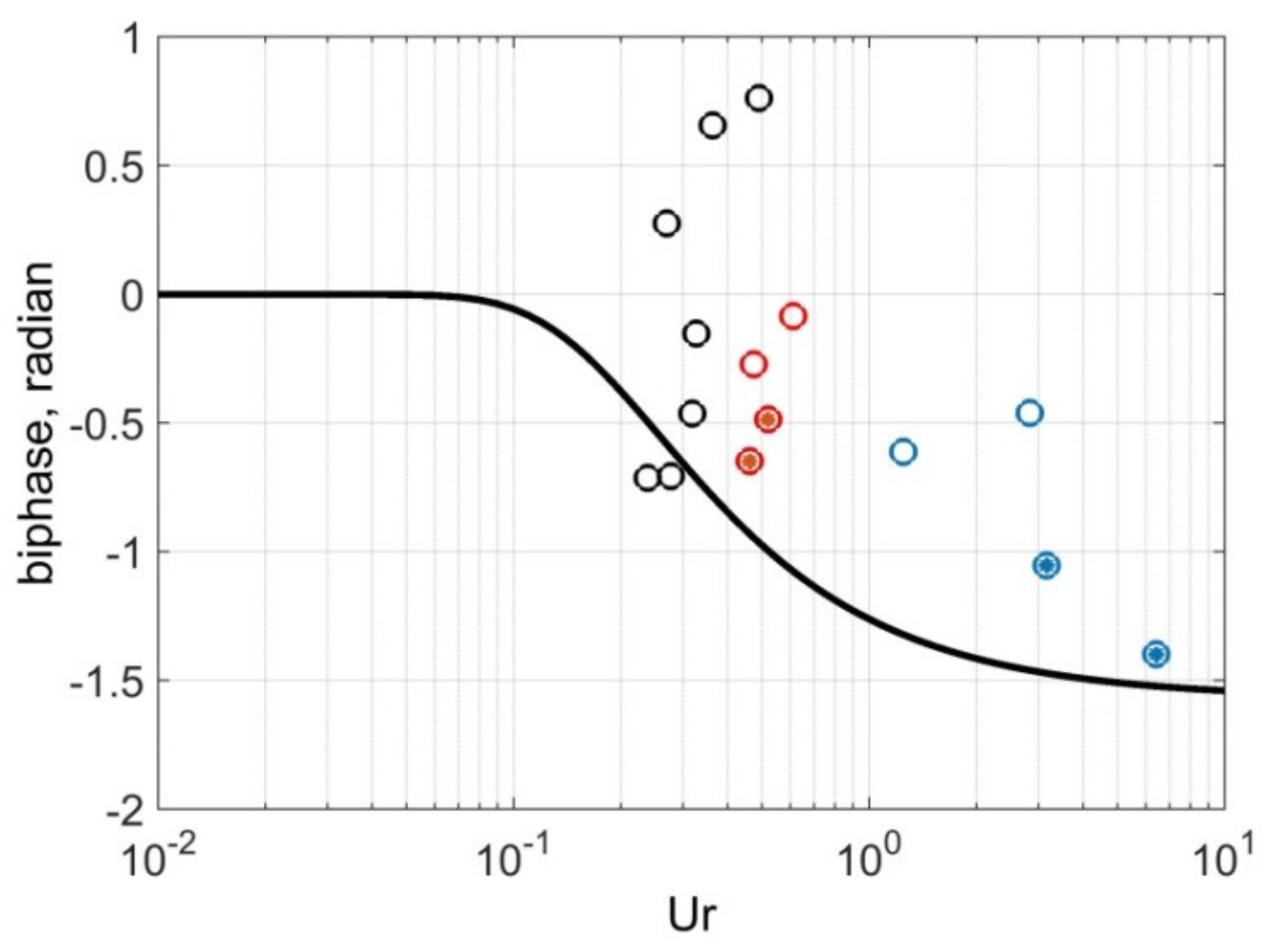
It is seen that in the LTA method the nonlinear contribution of the second harmonic is significantly higher, which is associated with the method of parametrization of nonlinear triad interactions. In the SPB method, the nonlinear changes for the 2nd and 3rd harmonics are similar to the Boussinesq model. The Boussinesq model gives a too-fast growth of the higher harmonics (for example, 4th), which requires its greater dissipation. An additional factor affecting the significant difference in the dissipation coefficient for plunging waves when simulating using the LTA method may be an inaccurate approximation of the phase shift (biphase) by the empirical formula [34]:
Biphase = π/2 (tanh (0.2/Ur – 1)
As can be seen from Figure 6, the biphases obtained from experimental data do not coincide well with this parameterization. The disadvantages of this parameterization of the Ursell number are discussed in more detail in [24].
The main reason for the inaccuracy of this parametrization is the neglect of visible periodic energy exchange between harmonics and the corresponding fluctuations of biphase (Figure 7), which arises as a consequence of the detuning in the wavenumber or near-resonance wave interaction, when the doubled wave number of the first harmonic is not equal to the wavenumber of the second harmonic and the amplitudes of the harmonics in the frequency domain are the result of the interference of amplitudes of several wave numbers or free and bound waves [23,37]. As can be seen from Figure 6 and Figure 7, those biphase values that correspond to the maximum of the second harmonic are significantly outside of the parameterization (see Equation (7)). For spilling breaking waves, the Ursell number is smaller, the deviation is smaller, and the results are similar. The SPB method, which takes into account the wave number detuning, turns out to be closer to the Boussinesq model.
To reduce the discrepancy in modeling, including due to incorrect parameterization, tuning of the model coefficients is widely used. Both SPB and LTA nonlinearity source models have an adjustable proportionality coefficient, trfac, with default values of 0.05 for LTA and 0.9 for SPB models [28]. The coefficient for LTA model has been recently adjusted from its previous default value of 0.8 [27]. The coefficient for 2D applications was calibrated in [36], resulting in a recommended value of 0.52 for the LTA model. The behavior of the SPB model can be further adjusted by calibrating the parameter K [35]:
K = 0.95kp − 0.75
where kp is the seaward peak wavenumber computed from the peak frequency, fp.
For this purpose, the SWAN model uses two coefficients a and b, which are related to the broadening of the resonance condition. The default values are recommended as a = 0.95 and b = 0.0 (for SPB). A sensitivity study is conducted by modifying trfac, a and b coefficients. However, b = −0.75 is recommended for the one-dimensional case. Then, a = 1, with default values of b = 0 and b = −0.5, and b = −0.75, with the default value of a = 0.95, are evaluated to calibrate the dissipation coefficient for the SPB method. The results are shown in Figure 8.
It is visible that trfac = 0.52 significantly decreases the frequency selectivity of wave energy dissipation for the LTA method. Dependence of the dissipation coefficient on frequency is approximately quadratic and qualitatively differs less than for the SPB method. Figure 8 also indicates that almost all SPB model parameterizations provide more uniform dissipation coefficients than the LTA model for both plunging and spilling breaking waves. The applicable range of a and b coefficients is very narrow in models with “no dissipation”. Model results varied slightly, with modifications to a and b coefficients, whereas they were impacted significantly by the modification of trfac. For the considered data, the results also revealed that the SPB model with trfac = 0.05 parametrization returned the most homogenous outputs for both spilling and plunging breaking waves, allowing the use of non-frequency-dependent energy dissipation formulations (bulk energy dissipation).
Another interesting finding is obtained for plunging breaking by the modification of the model parameters. Much greater dissipation is obtained around the first harmonic for trfac = 0.05 for both the SPB and LTA models.

4. Conclusions

We studied the necessary dissipation term for waves breaking by different types for modeling wave spectrum through phase-resolving and phase-averaged models with recommended default nonlinear terms. For this, the data from modeling with only linear and nonlinear terms (with switch-off dissipation term) and the data of the field experiment were compared. It was revealed that modeling the dissipation of wave energy during wave breaking in the phase-resolved and phase-averaged models should be carried out taking into account the compensation of nonlinear changes arising from the use of different nonlinear source terms.
It was found that spilling breaking waves have a dissipation coefficient with frequency selectivity at frequencies of the 2nd and 3rd harmonics, regardless of the types of spectral model and nonlinear term. The absence of significant differences is apparently due to the small contribution of nonlinearity to the change in the spectrum, since spilling breaking is characteristic of waves transforming over a gentle slope of the bottom.
For the plunging breaking waves, the quadratic dependence of the dissipation coefficient on the frequency is characteristic for the SPB method and for the Boussinesq model. For the LTA method with default parameters for plunging breaking waves as well as spilling breaking waves, there is a frequency-selective dissipation coefficient at a frequency of the 2nd harmonic. This is due to the insufficient accuracy of modeling non-linear processes by this method, including the inaccuracy of the biphase approximation.
It is possible to improve the accuracy of LTA and SPB methods by tuning the model coefficients. Thus, if parameter trfac = 0.52, LTA and SPB methods will give, on a qualitative level, similar results for quadratic frequency dependence of wave energy dissipation for plunging breaking waves.
The differences found show that, to increase the accuracy, it is also possible to have a different description of the dissipative term for waves breaking by different types. In this work, our goal was not to find the exact form of the dissipative term for improving the models, but to determine whether there are qualitative differences in modeling waves with different types of breaking, which was demonstrated. Therefore, as a further work, we will consider obtaining approximations for the dissipative term for waves breaking by spilling and plunging on the basis of a large array of data from field experiments.

Author Contributions

Conceptualization, methodology, Boussinesq modeling, analysis, draft writing, and writing—review and editing, Y.S.; SWAN modeling, writing—original draft preparation, B.A. (Burak Aydogan); analysis, writing—original draft preparation, writing—review and editing, B.A. (Berna Ayat). All authors have read and agreed to the published version of the manuscript.

Funding

This research was funded by RFBR and TUBITAK according to the joint research project 20-55-46005 and TUBITAK grant number 119N400.

Data Availability Statement

All experimental data are available from the authors by contacting [email protected] and [email protected].

Acknowledgments

This research was performed in the framework of the state assignment of the Institute of Oceanology of the Russian Academy of Sciences, theme No.0128-2021-0004.

Conflicts of Interest

The authors declare no conflict of interest.

References

  1. Saprykina, Y. The Influence of Wave Nonlinearity on Cross-Shore Sediment Transport in Coastal Zone: Experimental Investigations. Appl. Sci. 2020, 10, 4087. [Google Scholar] [CrossRef]
  2. Mase, H.; Kitano, T. Spectrum-based prediction model for random wave transformation over arbitrary bottom topography. Coast. Eng. J. 2000, 42, 111–151. [Google Scholar] [CrossRef]
  3. Kaihatu, J.; Kirby, J. Effects of mode truncation and dissipation on predictions of higher order statistics. Coast. Eng. Proc. 1996, 25, 123–135. [Google Scholar]
  4. Kirby, J.; Kaihatu, J. Structure of frequency domain models for random wave breaking. Coast. Eng. Proc. 1996, 25, 1144–1155. [Google Scholar]
  5. Madsen, P.A.; Sørensen, O.R. Bound waves and triad interactions in shallow water. Ocean Eng. 1993, 20, 359–388. [Google Scholar] [CrossRef]
  6. Eldeberky, Y.; Madsen, P.A. Determenistic and stochastic evolution equations for fully dispersive and weakly nonlinear waves. Coast. Eng. 1999, 38, 1–24. [Google Scholar] [CrossRef]
  7. Moris, J.; Catalán, P.; Cienfuegos, R. Incorporating wave-breaking data in the calibration of a Boussinesq-type wave model. Coast. Eng. 2021, 168, 103945. [Google Scholar] [CrossRef]
  8. Battjes, J.A.; Beji, S. Breaking waves propagating over a shoal. Coast. Eng. Proc. 1992, 23, 42–61. [Google Scholar]
  9. Beji, S.; Battjes, J.A. Experimental investigation of wave propagating over a bar. Coast. Eng. 1993, 19, 151–162. [Google Scholar] [CrossRef]
  10. Eldeberky, Y.; Battjes, J. Spectral modeling of wave breaking: Application to Boussinesq equations. J. Geophys. Res. 1996, 101, 1253–1264. [Google Scholar] [CrossRef]
  11. Mase, H.; Kirby, J. Hybrid Frequency-domain KDV equation for random wave transformation. Coast. Eng. Proc. 1992, 23, 474–487. [Google Scholar]
  12. Chen, Y.; Guza, R.; Elgar, S. Modeling spectra of breaking surface waves in shallow water. J. Geophys. Res. 1997, 102, 25035–25046. [Google Scholar] [CrossRef] [Green Version]
  13. Elgar, S.; Guza, R.T.; Raubenhaimer, B. Spectral evolution of shoaling and breaking waves on a barred beach. Geophys. Res. 1997, 102, 15797–15805. [Google Scholar] [CrossRef] [Green Version]
  14. Bredmose, H.; Schäffer, H.A.; Madsen, P.A. Boussinesq evolution equations: Numerical efficiency, breaking and amplitude dispersion. Coast. Eng. 2004, 51, 1117–1142. [Google Scholar] [CrossRef]
  15. Kaihatu, J.; El Safty, H.M. Spectral description of energy dissipation in breaking wave groups. Coast. Eng. Proc. 2011, 32, 19. [Google Scholar] [CrossRef] [Green Version]
  16. Kuznetsov, S.Y.; Saprykina, Y.V. Frequency-Dependent Energy Dissipation of Irregular Breaking Waves. Water Resour. 2004, 31, 384–392. [Google Scholar] [CrossRef]
  17. Meza, E.; Zang, J.; Seymour, R.J. Free-wave energy dissipation in experimental breaking waves. J. Phys. Oceanogr. 2000, 30, 2404–2418. [Google Scholar] [CrossRef]
  18. Antsyferov, S.M.; Kuznetsov, S.Y.; Saprykina, Y.V.; Kos’yan, R.D. Physical Grounds for the Formation of the Sediment Flux in the Coastal Zone of a Nontidal Sea. Oceanology 2005, 45, S183–S190. [Google Scholar]
  19. Herbers, T.H.C.; Russnogle, N.R.; Elgar, S. Spectral Energy Balance of Breaking Waves within the Surf Zone. J. Phys. Oceanogr. 2000, 30, 2723–2737. [Google Scholar] [CrossRef]
  20. Saprykina, Y.V.; Kuznetsov, S.Y.; Kuznetsova, O.A.; Shugan, I.V.; Chen, Y.Y. Wave Breaking Type as a Typical Sign of Nonlinear Wave Transformation Stage in Coastal Zone. Phys. Wave Phenom. 2020, 28, 75–82. [Google Scholar] [CrossRef]
  21. Salmon, J.E.; Holthuijsen, L.H.; Zijlema, M.; van Vledder, G.P.; Pietrzak, J.D. Scaling depth-induced wave-breaking in two-dimensional spectral wave models. Ocean Model. 2015, 87, 30–47. [Google Scholar] [CrossRef]
  22. Saprykina, Y.V.; Kuznetsov, S.Y.; Divinskii, B.V. Influence of processes of nonlinear transformations of waves in the coastal zone on the height of breaking waves. Oceanology 2017, 57, 383–393. [Google Scholar] [CrossRef]
  23. Saprykina, Y.V.; Kuznetsov, S.Y.; Shtremel, M.N.; Andreeva, N.K. Scenarios of nonlinear wave transformation in the coastal zone. Oceanology 2013, 53, 422–431. [Google Scholar] [CrossRef]
  24. Saprykina, Y.V.; Shtremel, M.N.; Kuznetsov, S.Y. On the possibility of biphase parametrization for wave transformation in the coastal zone. Oceanology 2017, 57, 253–264. [Google Scholar] [CrossRef]
  25. Borkowski, P. Numerical Modeling of Wave Disturbances in the Process of Ship Movement Control. Algorithms 2018, 11, 130. [Google Scholar] [CrossRef] [Green Version]
  26. Chizhiumov, S.D. Numerical Modeling of Ship Motion in Heavy Sea Conditions. In Proceedings of the Sixth ISOPE Pacific/Asia Offshore Mechanics Symposium, Vladivostok, Russia, 12–16 September 2004. [Google Scholar]
  27. The SWAN Team. SWAN User Manual—SWAN Cycle III Version 41.31A; Delft University of Technology: Delft, The Netherlands, 2020; p. 143. Available online: http://swanmodel.sourceforge.net/online_doc/swanuse/swanuse.html (accessed on 4 December 2021).
  28. The SWAN Team. User Manual SWAN—Cycle III version 41.31AB; Delft University of Technology: Delft, The Netherlands, 2021; p. 152. Available online: https://swanmodel.sourceforge.io/download/zip/swantech.pdf (accessed on 4 December 2021).
  29. Mei, C.C. The Applied Dynamics of Ocean Surface Waves; Wiley: New York, NY, USA, 1983; p. 740. [Google Scholar]
  30. Komen, G.J.; Cavaleri, L.; Donelan, M.; Hasselmann, K.; Hasselmann, S.; Janssen, P.A.E.M. Dynamics and Modelling of Ocean Waves; Cambridge University Press: Cambridge, UK, 1994; p. 532. [Google Scholar]
  31. Holthuijsen, L.H.; de Boer, S. Wave Forecasting for Moving and Stationary Targets. In Proceedings of the Computer Modelling in Ocean Engineering, Venice, Italy, 19–23 September 1988; Schrefler, B.A., Zienkewicz, O.C., Eds.; Taylor & Francis: London, UK; pp. 231–234. [Google Scholar]
  32. Eldeberky, Y. Nonlinear transformation of wave spectra in the nearshore zone. Commun. Hydr. Geotech. Eng. 1996, 96, 1–203. [Google Scholar]
  33. Booij, N.; Holthuijsen, L.H.; Bénit, M.P. A distributed collinear triad approximation in SWAN. In Proceedings of the Coastal Dynamics 2009: Impacts of Human Activities on Dynamic Coastal Processes (With CD-ROM), Tokyo, Japan, 7–11 September 2009; World Scientific: Singapore, 2009; pp. 1–10. [Google Scholar]
  34. Doering, J.C.; Bowen, A.J. Parameterization of orbital velocity asymmetries of shoaling and breaking waves using bispectral analysis. Coast. Eng. 1995, 26, 15–33. [Google Scholar] [CrossRef]
  35. Becq-Girard, F.; Forget, P.; Benoit, M. Non-linear propagation of unidirectional wave fields over varying topography. Coast. Eng. 1999, 38, 91–113. [Google Scholar] [CrossRef]
  36. Salmon, J.E.; Smit, P.B.; Janssen, T.T.; Holthuijsen, L.H. A consistent collinear triad approximation for operational wave models. Ocean Model. 2016, 104, 203–212. [Google Scholar] [CrossRef]
  37. Kuznetsov, S.; Saprykina, Y. Nonlinear Wave Transformation in Coastal Zone: Free and Bound Waves. Fluids 2021, 6, 347. [Google Scholar] [CrossRef]
Figure 1. Setup of field experiment and positions of wave breaking; wave gauges are marked by numbers.
Jmse 10 00200 g001
Figure 2. Wave spectra before and after wave breaking, field experiment (a) plunging breaking waves; (b) spilling breaking waves.
Jmse 10 00200 g002
Figure 3. Dissipation coefficients (Equation (1)) for wave breaking by plunging (a) and spilling (b) in dependence on the relation of frequency to spectral peak frequency (or number of nonlinear harmonics).
Jmse 10 00200 g003
Figure 4. Relative changes of wave spectra due to linear wave transformation only: (a) spilling breaking waves, (b) plunging breaking waves.
Jmse 10 00200 g004
Figure 5. Relative changes of wave spectra in modeling with excluded dissipation term: (a) spilling breaking waves, (b) plunging breaking waves.
Jmse 10 00200 g005
Figure 6. Biphase of waves (experiment) and parametrization curve (see Equation (7)). Filled circles correspond to points between points before and after wave breaking. Red: spilling breaking waves; blue: plunging breaking waves.
Jmse 10 00200 g006
Figure 7. Changes of amplitudes of first (a1) and second (a2) wave harmonics (a) and biphases (b) in the field experiment (see Figure 1).
Jmse 10 00200 g007
Figure 8. Adjustment of dissipation coefficients for plunging (a) and spilling (b) type wave breaking. In the legend, each parametrization is named after the modified parameters from the default setup. Parameters that are not indicated are kept as defaults.
Jmse 10 00200 g008
Publisher’s Note: MDPI stays neutral with regard to jurisdictional claims in published maps and institutional affiliations.

