Basic Ship-Planning Support System Using Big Data in Maritime Logistics for Simulating Demand Generation

Abstract

Dynamic changes in the global market demand affect ship development. Correspondingly, big data have provided the ability to comprehend the current and future conditions in numerous sectors and understand the dynamic circumstances of the maritime industry. Therefore, we have developed a basic ship-planning support system utilizing big data in maritime logistics. Previous studies have used a ship allocation algorithm, which only considered the ship cost (COST) along limited target routes; by contrast, in this study, a basic ship-planning support system is reinforced with particularized COST attributes and greenhouse gas (GHG) features incorporated into a ship allocation algorithm related to the International Maritime Organization GHG reduction strategy. Additionally, this system is expanded to a worldwide shipping area. Thus, we optimize the operation-level ship allocation using the existing ships by considering the COST and GHG emissions. Finally, the ship specifications demanded worldwide are ascertained by inputting the new ships instance.

1. Introduction

Economic growth creates dynamic changes in the global market, including the maritime industry. On a worldwide scale, huge demand for industrial cargo transport promotes intense ship movement and replacement [1]. As the demand for newbuilding specifications also changes according to the circumstances, developing a ship with adequate specifications to satisfy this demand is essential.

Meanwhile, the use of digital infrastructure to alter a business model and implement value-producing opportunities naturally generates a large data stream called big data. With the reduction in cost of data collection tools, a large amount of data can be obtained from various sources and formats [2,3]. This is significant for a broader understanding of the current and future conditions of various industries. Therefore, big data analytics will be a critical advantage in the future [4].

In the maritime industry, big data are being generated through advancements in navigation systems [5,6]. Together with the voyage data recorder, an automatic identification system (AIS) is required by the International Convention for the Safety of Life at Sea to aid navigation and avoid collisions of ocean-going ships. Towards its development, the deployment of satellite-based AIS receiver enables an accurate ship’s geospatial monitoring on a worldwide scale [7]. From the ship side, an AIS transponder also transmits a ship’s identification number, position, course, speed, and destination. These systems uphold the digitalization of previously analog-stored data, such as ship specifications, port limitations, and sailing routes [8].

The collection of static and dynamic big data in maritime logistics has allowed various studies to be conducted. Safety improvement, energy efficiency, logistics optimization, and predictive analysis have been broadly discussed [9,10,11,12]. Similarly, many data-driven studies have introduced a demand forecasting application for both regional and global scales. Forecasting analyses, such as the cargo throughput and shipbuilding market, have also been presented in some studies [13,14,15,16,17,18,19,20,21,22,23,24,25]; however, the demand for new ship specifications is unlikely to have been covered.

With big data in maritime logistics, ship operation monitoring is becoming relevant. Besides, shipbuilding tends to apply risk-based design rather than rules-based design, with aims of compatibility of design and performance [26,27]. Likewise, the International Maritime Organization (IMO) greenhouse gas (GHG) reduction strategy [28,29] set out a new future guideline. Therefore, it is crucial to examine the actual ship operation characteristics in the particular route to optimize its future ship design, both cost- and GHG-effectively.

Our prior studies examined the demand for new ship specifications by proposing a basic ship-planning support system using big data in maritime logistics [30]. We built the system and conducted the simulations in the form of a basic study. The proposed system was applied to the target ship of Capesize dry bulk carrier, which operated on relatively fixed routes, such as Australia and Brazil to East Asia routes [31]. Assuming the target ship operated in a time-charter contract manner, we built an algorithm to replicate its ship bidding scheme. However, the scope of that study was limited by the target routes and ship allocation considerations. The previous system delivered the simulations by only considering the ships’ fuel costs; by contrast, this study has proposed an enhancement to our basic ship-planning support system. Additionally, we have broadened the scope of the geographical area to a global scale to understand the ship specifications in demand. Finally, we suggest two attributes to be considered in the ship allocation algorithm: ship cost (COST) aspects and GHG emissions.

2. Literature Review

2.1. Related Studies Utilizing Big Data in Maritime Logistics

In recent years, studies utilizing big data in maritime logistics have emerged as a tool for predictive analytics. These have mainly discussed energy efficiency improvement, accident avoidance, and logistics optimization. Focusing on both regional and global scales, some studies have examined the forecasting of the cargo throughput, shipbuilding market, and new ship specifications [9,10,11,12]. Table 1 lists several studies on these topics.

Table 1. Related studies utilizing big data in maritime logistics.

Author	Forecasting Scope	Logistical Context 1	Shipping Market 2	Used Data 3
[13]	Cargo Throughput	Country	Co	Po
[14,15,16]	Cargo Throughput	Country	Co	Po, St
[17]	Cargo Throughput	Global	Bu	Ai
[18,19]	Cargo Throughput	Global	Bu	Ai, Sh
[20]	Shipping Market	Global	Ta	Ai, St
[21]	Shipbuilding Market	Global	Co, Bu, Ta	St
[22,23,24]	Shipbuilding Market	Global	Bu	Sh, St
[25]	Shipbuilding Market	Global	Co, Bu	Ai, Sh, St
[30]	New Ship Specification	Region	Bu	Sm, Sh, Po, Ro, St
This Study	New Ship Specification	Global	Bu	Sm, Sh, Po, Ro, St

¹Country: From or to a country; Region: Connections between more than two countries; Global: Worldwide scale; ²Co: Container; Bu: Bulk Carrier; Ta: Tanker; ³Ai: AIS data; Sm: ship movement data; Sh: ship data; Po: port data; Ro: route data; St: statistical data.

Regarding container throughput forecasting, Yang and Chang [13], Jugović et al. [14], Akar and Esmer [15], and Gökkuş et al. [16] constructed a long-term model predicting cargo demand based on regression analysis and neural networks using a combination of ship and port data. Moreover, Jia et al. [17] evaluated a regression model by inputting the AIS data of bulk carriers to estimate its payload and measure the future global carbon footprint per transport mode. Similarly, Zhou and Hu [18] examined an AIS-based estimation of iron ore volume. The actual shipment was obtained by inputting the static and dynamic data into the constructed back-propagation neural network. In addition, Kanamoto et al. [19] discussed the applicability of the AIS data of dry bulk carriers to forecast future shipping demand using a logit model.

For the case of shipping and newbuilding markets, Prochazka et al. [20] analyzed the effectiveness of AIS data to comprehend the behavior of the crude oil tanker spot-market charterer using quantile regression. Sharma and Sha [21] formulated a newbuilding index forecast based on neural networks and genetic algorithms using statistical data. Similarly, Wada et al. [22,23,24] suggested a system dynamics model to forecast the shipbuilding market demand, together with long-term GHG emissions reduction measures. Finally, Lee and Jung [25] built a platform to collect big data in shipbuilding and forecast the ship order quantity of container ships and bulk carriers, adopting an autoregressive model.

The abovementioned studies have discussed a macro-level forecasting model for fluctuations in the shipping and shipbuilding markets. However, they have not examined the operation-level demand forecasting to understand competitive ship specifications following market changes.

2.2. Optimization Studies in Ship Deployment and Contracts

Several studies proposed an optimization method in ship deployment and contracts. Zhang et al. [32] analyzed the cold chain shipping mode selection between containerized and bulk reefers. Adopting the value-based management, each ship is deployed considering the economic and environmental objectives. Similarly, Venturini et al. [33] discussed the berthing times and positioning optimization in container terminals. A novel mathematical formulation is introduced to integrate the berth allocation problem and sailing speed optimization. It aims to investigate the trade-off between fuel consumption reductions and dwelling time extension. Up to 40% potential GHG emissions reduction is reported compared with when the ship sails at its design speed. These studies reported the correlation between the ship’s sailing speed and GHG emissions.

Arslan and Papageorgiou [34] adopted multi-stage stochastic programming to deal with the bulk carrier renewal problem, focusing on ship-sizing and deployment. It was reported to provide the total cost reduction. Lin and Liu [35] developed a genetic algorithm to solve the tramp shipping routing problem of Handymax dry bulk carrier. The combined mathematical model was proposed to overcome ship allocation and cargo movement problems. These studies formulated a novel method to optimize the operation-level ship allocation. However, a particular case study of an actual ship allocation was not considered.

Yang et al. [36] discussed the diverse applications of AIS data, including the ship performance evaluation. Dynamic route planning in the Baltic Sea Region to reduce ship owners’ COST and GHG emissions was examined [37]. The reported benefit can surpass the cost in the proposed cost-benefit analysis by reducing sailed distances and GHG emissions. It proved the applicability of AIS data to evaluating the ship allocation in the specific region. Dynamic optimization was specified as a future research opportunity to attain the optimized ship allocation considering various routes and external factors.

Bai et al. [38] examined the potency of financial hedging and operational risk management strategies to overcome significant earning risks in the tramp shipping scheme. Ordinary least square regression and the Bayesian belief network were proposed to take into account the data of 31 tramp shipping companies, such as ship age, sailing distances, and AIS data. Operational risk management strategies were reported to mitigate bunker price and freight rate fluctuation risks effectively. It confirmed that ship allocation optimization is attainable utilizing big data in maritime logistics.

2.3. Originalities in This Study

According to our literature review, no study has been carried out on demand forecasting at the particular operational level to recognize the benefit of new ship specifications in the future. Therefore, Arifin et al. [30] proposed a basic ship-planning support system by integrating big data into maritime logistics (see Table 1). We have explored the possibility of simulating operation-level ship allocation and successfully built a ship allocation algorithm as the core of our system. The following improvements have been suggested to the aforementioned study:

• Target route and cargo type: Prior simulations [30] were executed on limited target routes and cargo types, such as the Australia, Brazil, Japan, and South Korea routes of iron ore. In contrast, this study has broadened the scope of simulations to accommodate iron ore and coal routes worldwide.
• Ship allocation algorithm: The key performance index (KPI) in the prior ship allocation algorithm [30] considered only the fuel cost as the COST variable. Therefore, the previously generated ship allocation simulation directly reflected the estimated fuel cost, which was a fraction of the actual COST. In this context, this study has proposed more realistic COST attributes [1], such as the costs of fuel, operation, depreciation, and stockpiling.

3. Basic Concept

3.1. Data Used in This Study

3.1.1. Ship Movement Data

This dataset presents dynamic data of the ship movement and its attributes. In this study, the port calling data of ships obtained from the Market Intelligence Network (MINT) database of IHS Markit Ltd. [39] are defined as the ship movement data, which provide the historical ship position in a port-level manner for various ship types. The data acquisition between the port calling data of MINT and the operation reports of the ship’s operator have been evaluated by Wada et al. [40]. More than 95% of the ship operation reports from 2015 to 2018 are covered in the ship movement data.

We then extracted the ship movement data of the Capesize dry bulk carriers, which are dry bulk carriers with a deadweight tonnage (DWT) of more than 100,000 [31]. The time range of the data was from January 2015 to May 2019. Initially, the ship movement data contained 328,670 entries, including calling types of anchorage, port, and terminal, which enclose the ships’ IMO and name, country of origin and destination, port of origin and destination, dates of arrival and departure, and draughts of arrival and departure. In this study, we aggregated the data into voyage records. They were defined as the set of a ship origin port’s departure data and destination port’s arrival data. Thus, any operation between these entries was considered an outlier by referring to Arifin et al. [30]. Later, the entry numbers were reduced to 36,849 entries of laden and ballast.

3.1.2. Ship Data

This dataset presents static data of the ships’ specifications. The ship data from the Sea-web Ships database of IHS Markit Ltd. (London, UK) were used in this study [41]. We downloaded the ship data of the Capesize dry bulk carriers (DWT of 100,000 or more) [31], for ships built from 1962 to 2021. This dataset contained 3253 entries, including the technical and non-technical attributes of ships, such as the IMO, name, built year, displacement, DWT, length, breadth, draught, design speed, main engine power, operator, technical manager, and registered owner.

3.1.3. Port Data

This dataset presents static data of the port and its specifications. The ship data from the Sea-web Ports of IHS Markit Ltd. and the IHS Fairplay Ports and Terminals Guide were used in this study [42,43]. We downloaded the worldwide port data served by dry bulk carriers containing 2529 entries, which included the variables of the ports’ latitude–longitude, size limitations of served ships, and handled cargo type.

3.1.4. Route Data

This dataset presents static data of the routes and its sailing distances. The distance table of the IHS Fairplay Ports and Terminals Guide was used in this study [43]. We extracted the worldwide sailing distances served by dry bulk carriers containing 17,030 entries.

3.2. System Configuration

Three distinct models and a ship allocation algorithm were assembled in our basic ship-planning support system, as shown in Figure 1. We modeled a global network model, cargo movement model, and ship model using the available big data in maritime logistics. The global network model defines the ports worldwide and their attributes in its sailing network. The cargo movement model covers an estimation of cargo movement between ports. The ship model includes each ship and its specifications and predicts the ships’ operation conditions.

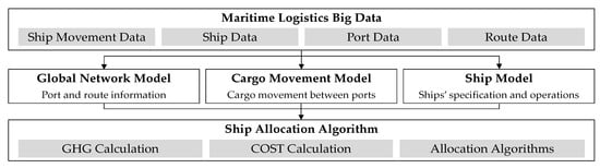
Figure 1. System configuration of this study.

The ship allocation algorithm reconstructs the ship allocation, which is the core of our basic ship-planning support system. An input of the cargo movement demand, route list, and existing ship list is needed to observe the changes in ship allocation by adding future scenarios, such as presenting the new ships in the ship list. Additionally, we can identify new ships that are replacing existing ships from their results, which makes it possible to assess competitive ships in demand.

3.2.1. Global Network Model

This model contains the ports’ specifications, sailing routes, and sailing distances. We extended its scope to include a worldwide sailing network served by Capesize dry bulk carriers. Thus, the model contained 564 ports and 1042 sailing routes. Additionally, we characterized the ports into main ports and port clusters.

3.2.2. Cargo Movement Model

This model provides the cargo movement and type between the ports. We used the arrival draught in the ship movement data to estimate the cargo amount. Later, this model results in various cargo movements arranged in origin–destination (OD) tables and is used as the cargo amount to be transported in the ship allocation algorithm.

3.2.3. Ship Model

This model depicts the ships’ specifications, which covers the technical and non-technical variables, such as the principal dimensions and ownership information. In addition, this model generates the operation conditions, draught rate, average sailing speed, and port staying time when a ship is allotted to a particular route. This model also predicts the operation conditions for each ship, which were later inputted into the GHG and COST calculations.

3.2.4. Ship Allocation Algorithm

This model computes the COST and GHG emissions when a ship is designated to a specific route. Then, this model allocates a ship onto a route with the highest merit to transport a certain cargo amount in a time-charter contract manner by adopting a greedy algorithm that considers the COST- and GHG-optimized ship allocation. Thus, this model optimizes the ship allocation and the global COST and GHG emissions, which are visualized in a region-level manner to understand the changes in the new ship allocation.

4. Model Development

4.1. Global Network Model

This model defines each port and route served by the Capesize dry bulk carriers. We extracted a list of ports visited by such carriers from the ship movement data on a worldwide scale. The various ports were divided into main ports and port clusters; the former represented each port with significant port calling numbers, and the latter included all the other ports served by the Capesize dry bulk carriers. The port and route network contains 52 main ports and 541 other ports as 79 port clusters, as shown in Figure 2.

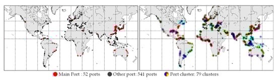
Figure 2. Worldwide ports of the global network model.

The main ports are mainly located in China (21 ports), Japan (7 ports), Australia (6 ports), and Brazil (4 ports) and accounted for 77.2% of the iron ore and coal trade in 2018, as seen from the worldwide port calling numbers of the Capesize dry bulk carriers [39], showing that most of the port calling numbers were served toward these countries. This tendency matches the worldwide top exporters and importers ranking of iron ore and coal in 2018 [31]. Additionally, this model also contains each port limitation and the sailing distance between the ports. The port limitations are set by port data and the largest possible ship visiting a port. Finally, the sailing distances were extracted from the IHS Fairplay Ports and Terminals Guide [43].

4.2. Cargo Movement Model

This model defines the worldwide port-to-port cargo movement demand served by the Capesize dry bulk carriers. This study defined the cargo movement demand between ports based on the estimated cargo movement (CARGO), which was calculated by considering the ship’s DWT and draught when it arrived at the destination port [30].

The set of available ships and routes of certain cargo types are represented as $I$ and $J$, respectively. The cargo movement ($C{M}_{ij}$) per trip for each ship $i$ serving the route $j$ (t), and the annual cargo movement ($C{A}_j$) of the route $j$ (t), are calculated as follows:

$$C{M}_{ij}=DW{T}_i\times \frac{\left(\raisebox{1ex}{${d^{\prime }}_{ij}$}\!\left/ \!\raisebox{-1ex}{$D_i$}\right.\right)}{\left(1-0.2\right)} \forall i\in I, \forall j\in J,$$

(1)

$$C{A}_j={{\displaystyle \sum }}_i\left(C{M}_{ij}\right) \forall i\in I, \forall j\in J,$$

(2)

where $DW{T}_i$ is the ship $i$ DWT, ${d^{\prime }}_{ij}$ is the ship $i$ arrival draught (m), and $D_i$ is the ship $i$ maximum draught (m). The $C{A}_j$ for each cargo type was collected later in the OD tables. Hence, these tables contained the annual cargo movement in a port-level manner.

This study classified the ship movement data into two voyage modes by referring to Arifin et al. [30]; laden and ballast. We applied Equation (1) to calculate the cargo movement ($C{M}_{ij}$) carried by ship $i$ only for its laden voyage. Then, the transported annual cargo movement ($C{A}_j$) is calculated by using Equation (2). It summarized all the laden instances in the route $j$ towards the target year. Finally, Table 2 shows a sample of the iron ore OD table. These data were used as the cargo movement demand in the ship allocation algorithm.

Table 2. A sample of iron ore origin–destination (OD) table.

Origin Ports	Destination Ports Cargo Movement (MT) 1
	Caofeidian	Zhoushan	Tianjin	Ningbo	Rizhao	Yingkou
Port Hedland	57.79	30.70	39.10	26.11	34.18	19.49
Itaqui	12.42	12.56	2.78	4.34	2.83	3.21
Tubarao	na	6.06	0.35	0.83	na	na

¹na: not available–no cargo movement.

4.3. Ship Model

4.3.1. Ship Specifications

This model contains each ship and its attributes. A ship is individually attached to several static variables as follows:

• Principal particulars: Length, breadth, and draught (m);
• Performance: Main engine power (kW) and design speed (kn);
• Administration: Shipbuilder, registered owner, manager, and operator.

4.3.2. Operation Condition Prediction

In addition to what has already been discussed, each ship is tied to its operation condition whenever a ship is assigned to a certain route. Therefore, it is necessary to know this information for all available routes. A ship’s operation conditions throughout a particular route are assumed to be its typical performance, despite of the actual contract. This study defines the operation conditions as follows:

• Draught rate: The ratio between the arrival draught and the ship’s design draught at the destination port;
• Average sailing speed: The ship’s average sailing speed starting from its departure time at the origin port to its arrival time at the destination port;
• Port staying time: The ship’s port staying time starting from its arrival time until its departure time at the destination port.

Figure 3 shows an overview of the proposed deep learning (DL) model. We constructed a DL model distinctively to predict the operation conditions in each voyage mode: laden and ballast. With each operation condition as the target feature, the model takes into account the following Capesize features as an input:

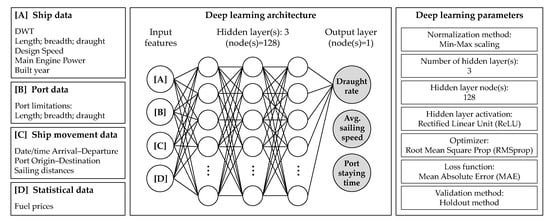
Figure 3. Deep learning (DL) model to predict operation conditions.

• Ship movement data [39,43]: 36,596 entries of worldwide operations from January 2015 to May 2019, which consist of dates of arrival and departure, ports of origin and destination, and sailing distances;
• Ship specifications [41]: 1658 entries, which consist of DWT, length, breadth, draught, design speed, main engine power, and built year;
• Port data [42]: 564 entries, which consist of port limitations of length, breadth, and draught.

The same architecture is used to predict the abovementioned operation conditions. Its input features are represented as binary vectors by using the one-hot encoding. These are normalized using Min-Max scaling before the training process.

The proposed DL model is comprised of three hidden layers of 128 nodes equipped with Rectified Linear Unit activation functions. We applied the optimizer of the Root Mean Square prop and the loss function of mean absolute error loss. Finally, we applied the holdout method to train our model, in which 70% was for the training data, 20% for the validation data, and 10% for the test data.

The average operation conditions of the worldwide routes (AVG) are the baselines that affirm the benefits of adopting the DL model. The DL prediction results, indicating a higher accuracy than the AVG, are shown in Table 3. Later, we will use the prediction results of the DL model to calculate the CARGO, GHG, and COST variables for each ship.

Table 3. Mean absolute error of DL model predictions.

Operation Condition	Mean Absolute Error of
	Deep Learning (DL) Model		Worldwide Average (AVG)
	Laden	Ballast	Laden	Ballast
Draught rate (%)	1.686	3.923	4.115	4.721
Avg. sailing speed (kn)	1.181	1.427	1.318	1.434
Port staying time (d)	1.273	2.439	1.819	3.129

5. GHG and COST Calculations

5.1. GHG Calculation

In this study, we calculated the total GHG, which has been referred to in prior IMO GHG studies [28,29]. It comprised the GHG emissions from the main engine and auxiliary machinery (an auxiliary engine and a boiler). This calculation used ship data and port data [41,42], as well as the results of the global network model and ship model. First, we calculated the actual power at which the main engine operated on average in sailing mode. The actual power of the main engine ($p_{ij}$) of a ship $i$ operating in the route $j$ (kW) is calculated as follows [28,29,32,33]:

$$p_{ij}=\frac{P_i\times {\left(\raisebox{1ex}{$d_{ij}$}\!\left/ \!\raisebox{-1ex}{$D_i$}\right.\right)}^{\left(\frac{2}{3}\right)}\times {\left(\raisebox{1ex}{$v_{ij}$}\!\left/ \!\raisebox{-1ex}{$V_i$}\right.\right)}^3}{\eta w_{ij}\times \eta f_{ij}} \forall i\in I, \forall j\in J,$$

(3)

where $P_i$ is the ship $i$ maximum main engine power (kW), $d_{ij}$ is the ship $i$ actual draught (m), $D_i$ is the ship $i$ maximum draught (m), $v_{ij}$ is the ship $i$ average sailing speed (kn), $V_i$ is the ship $i$ design speed (kn), and $\eta w_{ij}$ and $\eta f_{ij}$ are the correction factors of weather and fouling, respectively. The $P_i$, $D_i$, and $V_i$ of each ship were acquired from the ship data [41], $d_{ij}$ and $v_{ij}$ were generated by the ship model, and $\eta w_{ij}$ and $\eta f_{ij}$ were considered as constants with values 0.909 and 0.917, respectively [28]. After calculating $p_{ij}$, the main engine fuel consumption ($A_{ij}$) for a ship $i$ serving the route $j$ (t) is calculated as follows:

$$A_{ij}=\left(p_{ij}\times sf{c}_i\times s{t}_{ij}\right) \forall i\in I, \forall j\in J,$$

(4)

where $p_{ij}$ is the actual power of the main engine (kW), $sf{c}_i$ is the ship $i$ specific fuel oil consumption of the main engine (g/kWh), and $s{t}_{ij}$ is the round-trip sailing time (d). In this study, the main engine of ship $i$ was assumed to be a slow-speed diesel engine fueled by heavy fuel oil (HFO). Thus, $sf{c}_i$ for ships built before and after 2001 were assumed to be 185 and 175 g/kWh, respectively [28].

In addition to the main engine, we estimated the auxiliary machinery fuel consumption (an auxiliary engine and a boiler). The daily average fuel consumption of the auxiliary engine ($a_i$) and boiler ($b_i$) were determined by a linear correlation between the ship size and the average fuel consumption of the auxiliary machinery. The auxiliary machinery fuel consumption ($B_{ij}$) for a ship $i$ operating on the route $j$ (t) is calculated as follows:

$$B_{ij}=\left(a_i+b_i\right)\times s{t}_{ij} \forall i\in I, \forall j\in J,$$

(5)

where $a_i$ is the ship $i$ auxiliary engine daily average fuel consumption of the ship’s auxiliary engine (t/d), $b_i$ is the ship $i$ boiler daily average fuel consumption of the ship (t/d), and $s{t}_{ij}$ is the round-trip sailing time (d). Next, the possible annual trip ($n_{ij}$) of a ship $i$ serving the route $j$ is defined as follows:

$$n{x}_{ij}=\frac{\left(yd-m{d}_i\right)}{\left(s{t}_{ij}+p{s}_{ij}\right)}, n{y}_{ij}=\left(\frac{C{D}_{ij}}{C{M}_{ij}}\right) \forall i\in I, \forall j\in J,$$

(6)

$$n_{ij}=\{\begin{array}{c}n{x}_{ij} if \left(n{x}_{ij}\le n{y}_{ij}\right)\\ n{y}_{ij} if \left(n{x}_{ij}>n{y}_{ij}\right)\end{array} \forall i\in I, \forall j\in J,$$

(7)

where $n{x}_{ij}$ and $n{y}_{ij}$ are the possible annual trips considering the economic days and cargo movement, respectively. The $yd$ is the number of days in a year, taken as 365 (d), $m{d}_i$ is the assumed annual maintenance days (d), $s{t}_{ij}$ is the round-trip sailing time (d), $p{s}_{ij}$ is the loading–unloading time (d), $C{D}_{ij}$ is the annual transported cargo movement of route $j$ (t/y), and $C{M}_{ij}$ is the ship $i$ cargo movement per trip serving the route $j$ (t).

Finally, we define the total GHG emissions, which covered the GHG emissions of the main engine and auxiliary machinery. We calculate the annual GHG emissions ($G{H}_{ij}$) for a ship $i$ operating in the route $j$ (t) as follows:

$$G{H}_{ij}=\left(\left(A_{ij}\times CF\right)+\left(B_{ij}\times cf\right)\right)\times n_{ij} \forall i\in I, \forall j\in J,$$

(8)

where $A_{ij}$ is the main engine fuel consumption (t), $B_{ij}$ is the auxiliary machinery fuel consumption (t), $CF$ and $cf$ are the HFO and marine diesel oil (MDO) carbon factors (t-CO2/t-fuel), respectively, and $n_{ij}$ is the possible annual trip number. Following the IMO GHG study [28],$CF$ and $cf$ were taken as 3.114 and 3.206 t-CO2/t-fuel, respectively.

5.2. COST Calculation

In this study, the ship’s total COST considers the fuel, operation, depreciation, and stockpile costs [1]. The fuel cost represents the cost of the fuel needed to transport specific cargo from the origin port to the destination port. The operation cost describes the cost of operating the ship. It comprises the crew, consumables, repairs, and insurance costs. The depreciation cost defines the reduction in the ship resale price after a year of operation. The stockpile cost depicts the cost of stockpiling transported cargo at the destination port until the cargo is consumed based on the port’s daily cargo movement demand.

5.2.1. Fuel Cost Calculation

The fuel cost is calculated from the fuel consumption. The fuel cost ($F{C}_{ij}$) for a ship $i$ serving the route $j$ (USD) is calculated as the GHG emissions equation, by replacing the GHG emissions carbon factor ($CF,cf$) with fuel price constants ($FP,fp$), as follows:

$$F{C}_{ij}=\left(\left(A_{ij}\times FP\right)+\left(B_{ij}\times fp\right)\right) \forall i\in I, \forall j\in J,$$

(9)

where $A_{ij}$ is the main engine fuel consumption (t), $B_{ij}$ is the auxiliary machinery fuel consumption (t), and $FP$ and $fp$ are the HFO and MDO prices (USD/t-fuel), respectively. After observing the fluctuations in fuel prices [44], $FP$ and $fp$ were assumed to be 300 and 600 USD, respectively.

5.2.2. Operation Cost and Depreciation Cost Calculations

We composed response surfaces using the DWT and age of the dry bulk carrier ships to calculate the operation and depreciation costs. Considering Stopford [1], we expanded the correlation between the Capesize dry bulk carrier operation cost to other bulk carrier size classes [29,45,46]. Similarly, the depreciation cost was acquired by referring to the bulk carrier newbuilding and secondhand prices [44]. Figure 4a shows the daily operation cost for the given ship DWT and ship age which is defined by referring to the following attributes:

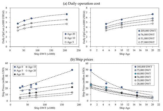
Figure 4. Bulk carrier (a) daily operation cost and (b) ship prices for the given ship DWT (left) and ship age (right).

• Daily operation cost of Capesize bulk carriers [1].
• Operation cost ratios of various bulk carrier size categories in 2011; Capesize, Panamax, Handymax, and Handysize [45].
• Ship DWT range for various bulk carrier size categories in 2011; Capesize, Panamax, Handymax, and Handysize [46].
• Average ship DWT for various bulk carrier size categories in 2011; Capesize (205,000 DWT), Panamax (76,000 DWT), Handymax (51,000 DWT), and Handysize (27,000 DWT) [29].

Correspondingly, the depreciation cost is determined by referring to the bulk carrier newbuilding and secondhand ship prices in 2019 [44]. The ship prices for the given ship DWT and ship age are shown in Figure 4b. The annual depreciation cost is obtained from the difference between the ship price in the current year and the previous year. Then, the daily depreciation cost was taken as annual depreciation cost divided by the number of days in a year, taken as 365 days. Finally, we represent these attributes into the bulk carrier operation cost and depreciation cost response surfaces, as shown in Figure 5.

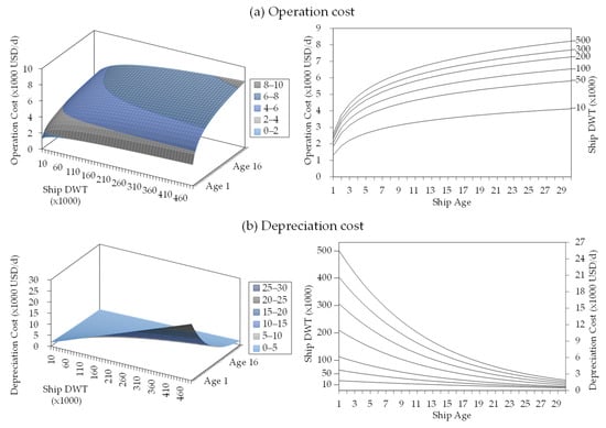
Figure 5. Response surfaces of bulk carrier (a) operation cost and (b) depreciation cost: 3D visualization (left) and 2D visualization (right).

Thus, the operation and depreciation costs ($O{C}_{ij},D{C}_{ij}$) for a ship $i$ operating in the route $j$ (USD) are calculated using the following equation:

$$O{C}_{ij}=\left(o{c}_i\times s{t}_{ij}\right), D{C}_{ij}=\left(d{c}_i\times yd\right) \forall i\in I, \forall j\in J,$$

(10)

where $o{c}_i$ is the ship $i$ daily operation cost (USD/d), $s{t}_{ij}$ is the round-trip sailing time (d), $d{c}_i$ is the ship $i$ daily depreciation cost (USD/d), and $yd$ is the number of days in a year (d), taken as 365. $o{c}_i$ and $d{c}_i$ for each ship $i$ are shown in Figure 5a,b, respectively, based on each ship’s DWT and age.

5.2.3. Stockpile Cost Calculation

Additionally, this study establishes the stockpile cost such that it resembles the cargo stockpile cost at the destination port. Origin and destination ports of route $j$ are defined as $k$ and $l$, respectively. The stockpile cost is determined by referring to the daily destination port cargo movement demand ($C{D}_l$, t/d), which is calculated as the sum of cargo movements (${{\displaystyle \sum }}_k^{ }\left(C{A}_{kl}\right)$) arriving at the destination port $l$ divided by 365 days ($yd$). Then, the accumulated period ($s{d}_{ij}$, d) is calculated by rounding off the division of cargo movement ($C{M}_{ij}$) carried by a ship $i$ to the destination port $l$ by the daily destination port cargo movement demand ($C{D}_l$) as follows:

$$C{D}_l=\left({{\displaystyle \sum }}_k^{ }\left(C{A}_{kl}\right)\right)\times \left(\frac{1}{yd}\right) \forall \left(j,l\right)\in J,$$

(11)

$$s{d}_{ij}=\frac{C{M}_{ij}}{C{D}_l} \forall i\in I, \forall \left(j,l\right)\in J.$$

(12)

Hence, the stockpile cost ($S{C}_{ij}$) for a ship $i$ serving the route $j$ (USD) is calculated as follows:

$$S{C}_{ij}=\left({{\displaystyle \sum }}_{x=0}^{s{d}_{ij}}C{M}_{ij}-\left(C{D}_l\times x\right)\right)\times s{c}_l \forall i\in I, \forall \left(j,l\right)\in J,$$

(13)

where $s{c}_l$ is the stockpile cost unit (USD/t/d), which depends on the port and cargo type. In this study, $s{c}_l$ was defined as a constant by referring to the average stockpile cost of the Japan Port Association [47]. Hence, $s{c}_l$ for iron ore and coal were taken as 0.012 and 0.042 USD/t/day, respectively.

5.2.4. Total COST Calculation

Finally, we define the total COST, which includes the fuel, operation, depreciation, and stockpile costs. The annual total COST ($T{C}_{ij}$) for a ship $i$ operating in the route $j$ (USD) is obtained as follows:

$$T{C}_{ij}=\left(\left(F{C}_{ij}+O{C}_{ij}+S{C}_{ij}\right)\times n_{ij}\right)+D{C}_{ij} \forall i\in I, \forall j\in J,$$

(14)

where $F{C}_{ij}$ is the fuel cost (USD), $O{C}_{ij}$ is the operation cost (USD), $S{C}_{ij}$ is the stockpile cost (USD), $D{C}_{ij}$ is the depreciation cost (USD), and $n_{ij}$ is the possible annual trip number. A sample of the COST composition is shown in Figure 6.

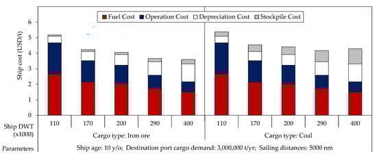
Figure 6. A sample of the COST composition.

5.3. Evaluation of GHG and COST Calculation

In this section, we will evaluate the GHG and COST calculation schemes. An evaluation of the GHG calculation is shown in Table 4. We calculated the main engine GHG emissions using the 2018 worldwide average ship age and draught rate of the Capesize dry bulk carriers [39] and the average variables depicted in the IMO GHG study [28]. For the following size categories, an error margin of less than 4% indicated the applicability of our GHG calculation scheme.

Table 4. Evaluation of GHG calculation.

Size Category (DWT ×1000)	GHG Emissions (MT)		Error (%)
	IMO GHG Study [28]	This Study
100–199	39.0	38.8	0.5
200–+	22.0	22.7	3.2

Similarly, Table 5 presents an evaluation of the COST composition with the following COST item parameters [1]:

Table 5. Evaluation of COST calculation.

COST Item	COST Composition (%)		Error (%)
	Stopford [1]	This Study
Fuel	35.2	34.4	0.7
Operation	16.2	20.3	4.1
Depreciation	48.6	45.3	3.3

• Fuel: 2005 HSFO 380cst and MDO Rotterdam bunker prices (USD) [44];
• Depreciation: 2005 daily depreciation cost (USD/d) [44];
• Ship: Operation conditions of a 10 year old ship in 2005 [41].

The error margin is between 0.7% and 4.1% for the COST item parameters, which justifies the practicability of our COST calculation scheme.

6. Ship Allocation Algorithm

6.1. Algorithm 1: Ship Replacement while Preserving the Existing Ship Allocation

Our algorithm proposes an optimization by offering a direct clone of the existing ship, which is a new ship with the exact specifications and operation conditions that serve the same annual allocations. The existing ship is replaced if the new ship offers practically lower COST or GHG emissions. Locally, a new ship justifies the replacement of an existing ship with the capability to reduce COST or GHG emissions. Globally, a collection of existing ships is replaced by new ship formations.

For each instance of an existing ship $i$, we offered a new ship $i^{\prime }$ with the same specifications, operation conditions, and annual allocations as the ship $i$ but with the admiralty coefficient of the year 2021. Additionally, we proposed two optimization schemes: COST- and GHG-optimized. In this section, we have provided an example of a COST-optimized case. Along with the calculation of the annual COST ($T{C}_{ij}$) per ton cargo ($C{M}_{ij}$) of a ship $i$, we also calculated the annual COST ($T{C}_{i^{\prime }j}$) per ton cargo ($C{M}_{i^{\prime }j}$) of an offered ship $i^{\prime }$. Thus, the KPI ($w_{ij},w_{i^{\prime }j}$) for each ship $i$ and $i^{\prime }$ serving the route $j$ is defined as follows:

$$w_{ij}=\left(\frac{T{C}_{ij}}{C{M}_{ij}}\right), w_{i^{\prime }j}=\left(\frac{T{C}_{i^{\prime }j}}{C{M}_{i^{\prime }j}}\right) \forall \left(i,i^{\prime }\right)\in I, \forall j\in J.$$

(15)

Finally, we acquired the global merit ($W_{ij}$), for an offered new ship $i^{\prime }$ replacing an existing ship $i$ by fulfilling the following conditions:

$$W_{ij}=\{\begin{array}{c}{w}_{ij} if \left(w_{ij}-w_{i^{\prime }j}\right)<0\\ w_{i^{\prime }j} if \left(w_{ij}-w_{i^{\prime }j}\right)>0\end{array} \forall \left(i,i^{\prime }\right)\in I, \forall j\in J,$$

(16)

where $W_{ij}$ represents a COST-effective ship. A ship $i^{\prime }$ is determined to replace the ship $i$ only if it offers a lower KPI. These steps resulted in a new ship allocation after conducting them for all the ships. Additionally, the seized COST reduction can be examined for an existing ship $i$ replaced by a new ship $i^{\prime }$.

6.2. Algorithm 2: An Optimization for Reconstructing Ship Allocation

Based on the greedy algorithm approach, this algorithm reconstructs the ship allocation to transport the worldwide cargo movement demand using the available ships in the existing allocation or with the new ships instance. Using the total COST and GHG emissions for each ship and route, the allocation algorithm transports the same cargo amount as the existing ship allocation in a time-charter contract manner. This algorithm allocates ships conforming to the limitations of port dimensions for certain ships.

A ship with the highest global merit is sequentially designated to transport cargo on a certain route on a one-year time-charter contract by replicating the ship bidding process to obtain the most advantageous ship. The allocation algorithm was adopted separately for both cases to achieve a global reduction in the total COST and GHG emissions. Next, we have provided an example of the ship allocation in the COST-optimized case only, since the allocation scheme for both the COST- and GHG-optimized cases are the same.

The annual COST ($T{C}_{ij}$) per ton cargo ($C{M}_{ij}$) was set as an individual ship KPI ($y_{ij}$). Additionally, the average KPI for the route $j$ (${\overline{y}}_j$) is known; therefore, the merit for each ship $i$ operating in the route $j$ ($m_{ij}$) is defined as follows:

$$y_{ij}=\left(\frac{T{C}_{ij}}{C{M}_{ij}}\right) \forall i\in I, \forall j\in J,$$

(17)

$$m_{ij}=\left({\overline{y}}_j-y_{ij}\right) \forall i\in I, \forall j\in J.$$

(18)

Finally, the global merit ($M$) is obtained as follows:

$$M=max\left(m_{ij}\right) \forall i\in I, \forall j\in J.$$

(19)

A set of ships and routes with the global merit $M$ is the most COST-effective allocation. Thereafter, the annual cargo movement demand of the route $j$ ($C{A}_j$) is subtracted by the annual cargo carried by that ship ($C{M}_{ij}$). The allocation algorithm is then repeated until all the cargo movement demands are assigned to a particular ship, while the allocated ship ($i$) is removed from the available ship list ($I$). All these processes result in the operation-level ship allocation. The annual CARGO, total COST, and GHG emissions were elaborated for each ship $i$ allotted on a specific route $j$. Therefore, we were able to explain the reduction in the total COST and GHG emissions and visualize the results geographically.

7. Case Studies and Discussions

We conducted several simulations using algorithms 1 and 2: ship replacement while preserving existing ship allocation (case study 1), optimization of ship allocation using existing ships (case study 2), and optimization of ship allocation using new ships instance (case study 3). First, we analyzed the actual ship allocation to understand the current ship allocation characteristics. Case study 1 analyzed new ships to replace existing ships without changing their allocation. Case study 2 reconstructed the ship allocation using only the existing ships. Case study 3 reconstructed the ship allocation using the existing ships and new ships instance (Table 6). Finally, we summarized the results of the average DWT and sailing speed graphically in a great circle format to give a better overview [48,49,50]. The following were the objectives of the simulations:

Table 6. Assumed specifications of the new ships.

New Ship	DWT	Draught (m)	Breadth (m)	Length (m)	Design Speed (kn)	Assumed Age	Existing M/E Power (kW) 1	New Ship M/E Power (kW) 1	M/E Power Reduction (%) 1
A	100,076	12.9	43.0	250	14.5	1	11,400	10,414	9.5%
B	183,194	18.2	45.0	292	14.5	1	15,815	15,317	3.2%
C	208,377	18.3	50.0	300	14.5	1	17,300	16,795	3.0%
D	261,046	18.8	57.0	327	14.5	1	22,324	19,446	14.8%
E	297,204	21.4	55.0	327	14.5	1	23,280	21,042	10.6%
F	403,508	23.0	65.0	361	14.5	1	29,260	25,583	14.4%

¹ M/E: main engine.

• Target ship: Capesize dry bulk carrier (DWT 100,000 or more, 1647 ships);
• Cargo types: Iron ore and coal;
• Route: Worldwide (sailing routes served by target ship);
• Operation period: 2018;
• Assumed fuel prices: 300 USD (HFO, $CF$) and 600 USD (MDO, $cf$).

7.1. Actual Ship Allocation

Before conducting simulations, it is necessary to analyze the typical features of the actual ship allocation. Figure 7 proportionally illustrates the ships’ average DWT and sailing speed, such that the line thickness indicates the annual cargo movement on each route, and the sorted colors represent the variance of the DWT and sailing speed.

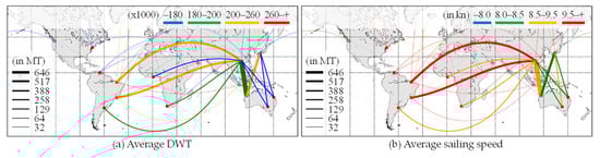
Figure 7. Actual ship allocation: (a) Average DWT and (b) sailing speed.

In the West Australia–China routes, which have the highest cargo movement, the average DWT is 180,000–200,000, and the average sailing speed is 8.5–9.5 knots, which indicates the use of smaller ships at typically slower speeds. Additionally, the long-distance routes, such as Brazil–China, show the ships operating with an average DWT of 200,000–260,000, and an average sailing speed exceeding 9.5 knots, which indicates that the routes are served by larger ships at higher speeds.

7.2. Case Study 1: Ship Replacement while Preserving the Existing Ship Allocation

7.2.1. Definition of Case Study 1

This case study attempted to directly replace each existing ship with a new ship without changing the actual ship allocation, and then to observe the changes in the total COST and GHG emissions, including COST-optimized ship replacement while preserving the existing ship allocation (case study 1a) and GHG-optimized ship replacement while preserving the existing ship allocation (case study 1b). The following were the parameters of case study 1:

• Method: Allocation algorithm 1;
• Offered ships: A new ship for each existing ship in the actual ship allocation.

We offered new ships with the same principal particulars but with the admiralty coefficient of 2021.

7.2.2. Results of Case Study 1

The allocated new ship rates for cases 1a and 1b are shown in Figure 8. Both the cases show a typically high allocation rate for new ships. Figure 8a shows the major routes that the allotted new ships take for over 40%–60% of the operation numbers. Meanwhile, Figure 8b shows that the new ships accounted for more than 60% of the worldwide operation numbers.

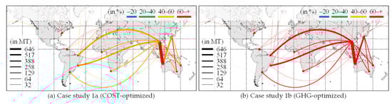
Figure 8. Ship replacement while preserving existing ship allocation: Allocated new ship rate of (a) case study 1a (COST-optimized) and (b) case study 1b (GHG-optimized).

As shown in Table 7, minor reductions in the total COST and GHG emissions can be seen in case study 1. In case study 1a, new ships replaced 58.8% of the total number of existing ship operations, which reduced the total COST by 3.5%, and the GHG emissions were reduced by 5.6% compared to the actual ship allocation. Moreover, case study 1b allotted 87.5% of its operations to new ships, which allowed a 9.7% reduction in the GHG emissions, but the total COST increased by 0.4%.

Table 7. Results of case studies.

Case Studies	Total COST in Million USD (Reduction in %)	GHG Emissions in MT (Reduction in %)	Total Operation Numbers (Reduction in %)	Operation Number of Allocated New Ships (%) 1
Actual ship allocation	10,847.8 (0.0%)	34.9 (0.0%)	9185 (0.0%)	na
Case study 1a (COST-optimized)	10,469.0 (3.5%)	33.0 (5.6%)	9185 (0.0%)	58.8%
Case study 1b (GHG-optimized)	10,883.4 (−0.4%)	31.6 (9.7%)	9185 (0.0%)	87.5%
Case study 2a (COST-optimized)	10,062.7 (7.3%)	32.7 (6.6%)	9091 (1.1%)	na
Case study 2b (GHG-optimized)	10,248.6 (5.6%)	29.8 (14.8%)	8989 (2.2%)	na
Case study 3a (COST-optimized)	9826.6 (9.5%)	30.3 (13.3%)	8246 (10.3%)	40.9%
Case study 3b (GHG-optimized)	11,345.2 (−4.6%)	27.0 (22.8%)	7560 (17.7%)	48.2%

¹na: not available–no new ship in the ship allocation.

7.3. Case Study 2: Ship Allocation Optimization Using Existing Ships

7.3.1. Definition of Case Study 2

In this case study, we discussed optimizing the ship allocation using only the existing ships. The two case studies covered are: COST-optimized ship allocation using existing ships (case study 2a) and GHG-optimized ship allocation using existing ships (case study 2b). The following were the parameters for case study 2:

• Method: Allocation algorithm 2;
• Offered ships: The existing ships operated in the current ship allocation.

7.3.2. Results of Case Study 2

The results obtained for case study 2 are illustrated in Figure 9. From Figure 9a, we can ascertain that the Brazil–China routes allotted larger ships with a DWT of more than 260,000 and an average sailing speed of more than 9.5 knots. The average DWT of ships designated to the Brazil–China routes increased, compared to the actual ship allocation, due to the use of larger ships.

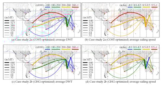
Figure 9. Ship allocation optimization using existing ships: Case study 2a (COST-optimized) (a) average DWT and (b) sailing speed; case study 2b (GHG-optimized) (c) average DWT and (d) sailing speed.

In Figure 9b, the major routes are allocated to ships with an average sailing speed of 8.5–9.5 knots. Subsequently, Figure 9c depicts a similar average DWT as the actual ship allocation, and the average sailing speed shown in Figure 9d is generally slower. This analysis indicated the importance of speed reduction in optimizing the fuel consumption and GHG emissions of the ships.

As summarized in Table 7, case study 2a reduced the total COST by 7.3% compared to the actual ship allocation, whereas the total GHG emissions were reduced by 14.8% in case study 2b. Additionally, the ship operation numbers of case studies 2a and 2b were reduced by 1.1% and 2.2%, respectively. Such changes in the ship allocation were made possible by the operation-level alterations, despite simply employing the existing ships. Nevertheless, a significant reduction in the total COST and GHG emissions could not be obtained using only the existing ships.

7.4. Case Study 3: Ship Allocation Simulation with New Ships Instance

7.4.1. Definition of Case Study 3

In addition to the analysis of case study 2 (Section 7.3), this case study presents a set of new ships. We examined the competitive new ships that could potentially replace the existing ships by conducting simulations to optimize the ship allocation with these new ships. The following were the parameters of case study 3:

• Method: Allocation algorithm 2;
• Offered ships: The existing ships of case study 2 and new ships.

The new ship specifications were sampled from the existing ships of the 2018 ship allocation. The set of sampled ships is defined as $S$. We defined these ships as more efficient since they had the admiralty coefficient of the year 2021: 697.29 ($AD{M}_{2021}$), as shown in Figure 10.

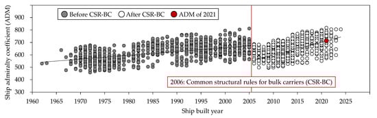
Figure 10. Ship admiralty coefficient (ADM) before and after common structural rules for bulk carriers (CSR-BC) [41,51,52].

Hence, the main engine power ($P_s^{\prime }$) was reduced by retaining a constant ship $s$ design speed as follows [51]:

$$P_s^{\prime }=P_s\times \left(\frac{AD{M}_s}{AD{M}_{2021}}\right) \forall s\in S,$$

(20)

where $P_s$ is the main engine power of ship $s$ (kW) and $AD{M}_s$ is the admiralty coefficient of ship $s$. Table 6 lists the specifications of the new ships. These ships had the same principal particulars as the sampled ships but lower main engine power. As new ships could be allotted indefinitely, we discussed the following case studies: COST-optimized ship allocation with new ships instance (case study 3a) and GHG-optimized ship allocation with new ships instance (case study 3b).

7.4.2. Results of Case Study 3

This case study optimized the ship allocation by allowing the existing ships to be replaced by new ships. This allowed us to ascertain the average DWT and sailing speed patterns simultaneously on a global scale. Figure 11 shows the ship allocation results of case study 3. From Figure 11a,c, we can observe that both the case studies allocated ships with a similar average DWT. The major routes displayed in Figure 11b have a uniform average sailing speed of more than 8.5 knots, similar to case study 2. The allocated ships’ lower average sailing speed compared to the actual ship allocation can be seen in Figure 11d. The short- and long-distance routes allocated ships with an average sailing speed of less than 8.5 knots and 8.5–9.5 knots, respectively. This indicated that the importance of sailing speed varied depending on the sailing distance.

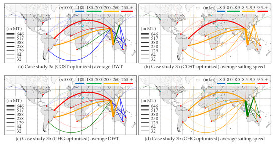
Figure 11. Ship allocation optimization with new ships instance: Case study 3a (COST-optimized) (a) average DWT and (b) sailing speed; case study 3b (GHG-optimized) (c) average DWT and (d) sailing speed.

In Table 7, we observe that case study 3a reduces the total COST by 9.5% compared to the actual ship allocation. These reductions were accounted for by new ships, replacing 40.9% of the existing operations. In case study 3b, the GHG emissions were reduced by 22.8%, but the total COST increased by 4.6%. To conclude, we identified a significant reduction in the total COST and GHG emissions by adding new ships.

7.5. Discussion 1: Significance of the Total COST and GHG Emissions Reductions

The results of each case study are compiled in Table 7. The case studies 1a and 1b employed new ships covering 58.8% and 87.5%, respectively, of the worldwide operation numbers using allocation algorithm 1. However, only minor changes were typically observed compared to the actual ship allocation, with a 3.5% total COST reduction in case study 1a and a 9.7% GHG emissions reduction in case study 1b.

Case study 2 optimized the ship allocation using only the existing ships operating in the current ship allocation by deploying allocation algorithm 2. Case study 2a realized a 7.3% total COST reduction, two times that of case study 1a, compared to the actual ship allocation. For the GHG emissions aspect, case study 2b achieved a 14.8% reduction, which was 1.5 times that of case study 1b. A more significant reduction in the total COST and GHG emissions was achieved by case study 2 than case study 1.

Case study 3 proposed new ships in the application of allocation algorithm 2 under the same constraints as that of case study 2. The new ships were defined as being able to be allocated indefinitely, which allowed such ships with higher merits to replace the existing ships as needed. In case study 3a, 40.9% of the operation numbers were served by the new ships, allowing a 9.5% total COST reduction compared to the actual ship allocation. For GHG emissions, 48.2% of the operation numbers in case study 3b were served by the new ships. This enabled a considerable reduction of 22.8% in the GHG emissions. Additionally, case study 3 allocated new ships at a considerably lower rate than case study 1. Nevertheless, the most significant reduction in the total COST and GHG emissions were actualized by presenting the new ships for the ship allocation optimization.

7.6. Discussion 2: New Ship Demand

In the previous section, case study 3 specified that notable results could be obtained by optimizing the ship allocation with the new ships instance. The allocated new ship rates of case studies 3a and 3b are shown in Figure 12. The allocated new ship rate was observed to vary depending on the sailing distance. Similarly, in the COST- and GHG-optimized cases, more than 60% of the new ships were allocated in the West Australia–China routes, the major iron ore routes with 646 million tons of cargo movement demands.

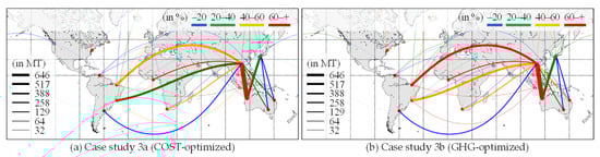
Figure 12. Ship allocation optimization with new ships instance: Allocated new ship rate of (a) case study 3a (COST-optimized) and (b) case study 3b (GHG-optimized).

Next, we examined the distinct specifications of the demanded new ships in the West Australia–China routes. Figure 13 shows the composition of operations in the COST- and GHG-optimized ship allocations with the new ships instance. The new ship E (DWT 290,000) was the most allocated, accounting for 47.9% and 54.7% of the operations of the COST- and GHG-optimized ship allocation, respectively.

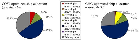
Figure 13. COST- and GHG-optimized ship allocation with new ships instance (case study 3): Composition of operations in the routes of West Australia–China.

This proved that the new ship E specification improvement, through the admiralty coefficient of 2021, presented a larger benefit than the existing ships in both the optimization cases. Moreover, looking at the significant main port restrictions of West Australia–China (Table 8), the largest new ship that entered was the new ship E, thus confirming that the demanded ship was a large iron ore bulk carrier.

Table 8. Significant main port limitations of West Australia and China.

Region	Port Name	Cargo Throughput (MT)	Length (m)	Breadth (m)	Draught (m)
West Australia	Port Hedland	386.8	340.0	57.0	25.5
	Dampier	124.0	330.1	57.0	25.5
	Port Walcott	118.1	330.1	57.0	25.5
China	Caofeidian	77.8	362.0	65.0	24.3
	Jingtang	71.7	333.0	60.0	25.5
	Zhoushan	66.1	362.0	65.0	23.3
	Tianjin	62.1	340.0	60.0	22.2
	Rizhao	50.5	340.0	62.0	22.6

8. Concluding Remarks

In this study, we have proposed an enhancement to our basic ship-planning support system. We expanded the scope of our simulations to a worldwide scale, which allowed a broad comprehension of the demand ship specifications. In addition, we developed a ship allocation algorithm to consider the detailed COST and GHG emissions attributes. The system itself consisted of three distinct models and an algorithm to resemble the ship allocation bidding process: a global network model, cargo movement model, ship model, and ship allocation algorithm. The global network model defined the main ports and port clusters, which resulted in the following: a cluster of ports and their attributes, port and route limitations, and sailing distances. The cargo movement model specified the cargo movement and cargo types between the ports. The ship model represented each ship and its specifications. This model predicted the operating conditions: draught rate, average sailing speed, and port staying time for each ship serving a particular route.

Ultimately, as the core of our system, the ship allocation algorithm reconstructed the operation-level ship allocation. It calculated COST and GHG emissions for each ship and a greedy algorithm mechanism was used to resemble the ship allocation. This study proposed two algorithms: ship replacement while preserving the existing ship allocation and an optimization for reconstructing the ship allocation. Allocation algorithm 1 offered a new ship with enhanced performance for each existing ship without changing the current ship allocation. Additionally, we reallocated the ship by applying allocation algorithm 2, which optimized the total COST and GHG emissions. We conducted two discrete simulations: optimization using only the existing ships operating in the actual ship allocation and with new ships instance. The ship allocation optimization indicated that significant reductions in the total COST and GHG emissions were not achievable using only the existing ships. Using the developed system, we were able to recreate an operation-level ship allocation considering various scenarios. Finally, we confirmed the demanded new ship specifications by presenting the new ships instance. However, this study is only feasible for the current constraints of the Capesize dry bulk carrier operating in the time-charter contract, despite the presented results. The application of the proposed system for other dry bulk carrier size categories such as Panamax and Handymax, and the voyage-charter contracts are considered future tasks. Likewise, considering the importance of weather routing, the weather correction factor in the main engine actual power calculation, which was previously assumed constant, is possibly varied [53]. Hence, further studies are crucial to assess the applicability of our system beyond these limitations.

References

- Stopford, M. Maritime Economics 3e; Routledge: Oxford, UK; New York, NY, USA, 2008. [Google Scholar]
- Fan, J.; Han, F.; Liu, H. Challenges of Big Data analysis. Natl. Sci. Rev. 2014, 1, 293–314. [Google Scholar] [CrossRef] [PubMed]
- Alharthi, A.; Krotov, V.; Bowman, M. Addressing barriers to big data. Bus. Horiz. 2017, 60, 285–292. [Google Scholar] [CrossRef]
- Saggi, M.K.; Jain, S. A survey towards an integration of big data analytics to big insights for value-creation. Inf. Process. Manag. 2018, 54, 758–790. [Google Scholar] [CrossRef]
- IMO. AIS Transponders. Available online: https://www.imo.org/en/OurWork/Safety/Pages/AIS.aspx (accessed on 28 September 2021).
- Svanberg, M.; Santén, V.; Hörteborn, A.; Holm, H.; Finnsgård, C. AIS in maritime research. Mar. Policy 2019, 106, 103520. [Google Scholar] [CrossRef]
- Bauk, S. A Review of NAVDAT and VDES as Upgrades of Maritime Communication Systems. Adv. Mar. Navig. Saf. Sea Transp. 2019, 13, 81–82. [Google Scholar] [CrossRef]
- IMO. Voyage Data Recorders. Available online: https://www.imo.org/en/OurWork/Safety/Pages/VDR.aspx (accessed on 28 September 2021).
- Munim, Z.H.; Dushenko, M.; Jimenez, V.J.; Shakil, M.H.; Imset, M. Big data and artificial intelligence in the maritime industry: A bibliometric review and future research directions. Marit. Policy Manag. 2020, 47, 577–597. [Google Scholar] [CrossRef]
- Mirović, M.; Miličević, M.; Obradović, I. Big data in the maritime industry. NAŠE MORE Znan. Časopis Za More I Pomor. 2018, 65, 56–62. [Google Scholar]
- Zaman, I.; Pazouki, K.; Norman, R.; Younessi, S.; Coleman, S. Challenges and Opportunities of Big Data Analytics for Upcoming Regulations and Future Transformation of the Shipping Industry. Procedia Eng. 2017, 194, 537–544. [Google Scholar] [CrossRef]
- Sanchez-Gonzalez, P.-L.; Díaz-Gutiérrez, D.; Leo, T.J.; Núñez-Rivas, L.R. Toward Digitalization of Maritime Transport? Sensors 2019, 19, 926. [Google Scholar] [CrossRef]
- Yang, C.-H.; Chang, P.-Y. Forecasting the Demand for Container Throughput Using a Mixed-Precision Neural Architecture Based on CNN–LSTM. Mathematics 2020, 8, 1784. [Google Scholar] [CrossRef]
- Jugović, A.; Komadina, N.; Hadžić, A.P. Factors influencing the formation of freight rates on maritime shipping markets. Pomorstvo 2015, 29, 23–29. [Google Scholar]
- Akar, O.; Esmer, S. Cargo Demand Analysis of Container Terminals in Turkey. J. ETA Marit. Sci. 2015, 3, 117–122. [Google Scholar] [CrossRef]
- Gökkuş, Ü.; Yıldırım, M.S.; Aydin, M.M. Estimation of Container Traffic at Seaports by Using Several Soft Computing Methods: A Case of Turkish Seaports. Discret. Dyn. Nat. Soc. 2017, 2017, 2984853. [Google Scholar] [CrossRef]
- Jia, H.; Prakash, V.; Smith, T. Estimating vessel payloads in bulk shipping using AIS data. Int. J. Shipp. Transp. Logist. 2019, 11, 25–40. [Google Scholar] [CrossRef]
- Zhou, X.; Hu, Q. Estimation of Shipment Size in Seaborne Iron Ore Trade. TransNav Int. J. Mar. Navig. Saf. Sea Transp. 2019, 13, 791–796. [Google Scholar] [CrossRef]
- Kanamoto, K.; Murong, L.; Nakashima, M.; Shibasaki, R. Can maritime big data be applied to shipping industry analysis? Focussing on commodities and vessel sizes of dry bulk carriers. Marit. Econ. Logist. 2021, 23, 211–236. [Google Scholar] [CrossRef]
- Prochazka, V.; Adland, R.; Wolff, F.-C. Contracting decisions in the crude oil transportation market: Evidence from fixtures matched with AIS data. Transp. Res. Part A Policy Pract. 2019, 130, 37–53. [Google Scholar] [CrossRef]
- Sharma, R.; Sha, O.P. Development of an Integrated Market Forecasting Model for Shipping and Shipbuilding Parameters. In Proceedings of the RINA–International Conference on Computer Applications in Shipbuilding, Portsmouth, UK, 18–20 September 2007; pp. 18–20. [Google Scholar]
- Wada, Y.; Yamamura, T.; Hamada, K.; Wanaka, S. Evaluation of GHG Emission Measures Based on Shipping and Shipbuilding Market Forecasting. Sustainability 2021, 13, 2760. [Google Scholar] [CrossRef]
- Wada, Y.; Hamada, K.; Hirata, N. Shipbuilding capacity optimization using shipbuilding demand forecasting model. J. Mar. Sci. Technol. 2021, 1–19. [Google Scholar] [CrossRef]
- Wada, Y.; Hamada, K.; Hirata, N.; Seki, K.; Yamada, S. A system dynamics model for shipbuilding demand forecasting. J. Mar. Sci. Technol. 2018, 23, 236–252. [Google Scholar] [CrossRef]
- Lee, S.; Jung, I. Development of a Platform Using Big Data-Based Artificial Intelligence to Predict New Demand of Shipbuilding. J. Inst. Internet Broadcasting Commun. 2019, 19, 171–178. [Google Scholar]
- Fujikubo, M. Digital Twin for Ship Structures: Research Project in Japan (Plenary Lecture Presentation). In Proceedings of the 14th International Symposium on Practical Design of Ships and Other Floating Structures, Yokohama, Japan, 22–20 September 2019. [Google Scholar]
- Breinholt, C.; Ehrke, K.-C.; Papanikolaou, A.; Sames, P.C.; Skjong, R.; Strang, T.; Vassalos, D.; Witolla, T. SAFEDOR–The Implementation of Risk-based Ship Design and Approval. Procedia Soc. Behav. Sci. 2012, 48, 753–764. [Google Scholar] [CrossRef][Green Version]
- Faber, J.; Hanayama, S.; Zhang, S.; Pereda, P.; Comer, B.; Hauerhof, E.; Yuan, H. Fourth IMO Greenhouse Gas Study. Available online: https://docs.imo.org (accessed on 28 September 2021).
- Smith, T.W.P.; Jalkanen, J.P.; Anderson, B.A.; Corbett, J.J.; Faber, J.; Hanayama, S.; O’keeffe, E.; Parker, S.; Johanasson, L.; Aldous, L.; et al. Third IMO Green House Gas study 2014; International Maritime Organization: London, UK, 2015. [Google Scholar]
- Arifin, M.D.; Hamada, K.; Hirata, N.; Ihara, K.; Koide, Y. Development of Ship Allocation Models using Marine Logistics Data and its Application to Bulk Carrier Demand Forecasting and Basic Planning Support. J. Jpn. Soc. Nav. Arch. Ocean Eng. 2018, 27, 139–148. [Google Scholar] [CrossRef]
- Sirimanne, S.N.; Hoffman, J.; Juan, W.; Asariotis, R.; Assaf, M.; Ayala, G.; Benamara, H.; Chantrel, D.; Hoffmann, J.; Premti, A. Review of maritime transport 2019. In Proceedings of the United Nations Conference on Trade and Development, Geneva, Switzerland, 31 January 2020. [Google Scholar]
- Zhang, X.; Lam, J.S.L.; Iris, Ç. Cold chain shipping mode choice with environmental and financial perspectives. Transp. Res. Part D Transp. Environ. 2020, 87, 102537. [Google Scholar] [CrossRef]
- Venturini, G.; Iris, Ç.; Kontovas, C.A.; Larsen, A. The multi-port berth allocation problem with speed optimization and emission considerations. Transp. Res. Part D Transp. Environ. 2017, 54, 142–159. [Google Scholar] [CrossRef]
- Arslan, A.N.; Papageorgiou, D.J. Bulk ship fleet renewal and deployment under uncertainty: A multi-stage stochastic programming approach. Transp. Res. Part E Logist. Transp. Rev. 2017, 97, 69–96. [Google Scholar] [CrossRef]
- Lin, D.-Y.; Liu, H.-Y. Combined ship allocation, routing and freight assignment in tramp shipping. Transp. Res. Part E Logist. Transp. Rev. 2011, 47, 414–431. [Google Scholar] [CrossRef]
- Yang, D.; Wu, L.; Wang, S.; Jia, H.; Li, K.X. How big data enriches maritime research–A critical review of Automatic Identification System (AIS) data applications. Transp. Rev. 2019, 39, 755–773. [Google Scholar] [CrossRef]
- Andersson, P.; Ivehammar, P. Dynamic route planning in the Baltic Sea Region–A cost-benefit analysis based on AIS data. Marit. Econ. Logist. 2017, 19, 631–649. [Google Scholar] [CrossRef]
- Bai, X.; Cheng, L.; Iris, Ç. Data-driven financial and operational risk management: Empirical evidence from the global tramp shipping industry. Transp. Res. Part E Logist. Transp. Rev. 2022, 158, 102617. [Google Scholar] [CrossRef]
- IHS MARKIT/TheTradeNet Market Intelligence Network (MINT). Available online: https://www.marketintelligencenetwork.com/ (accessed on 28 September 2021).
- Wada, Y.; Hamada, K.; Kamata, T.; Nanao, J.; Watanabe, D.; Majima, T. Evaluation of AIS data and port calling data using ship operation data of a shipping company. In Proceedings of the International Association of Maritime Economists (IAME), Hong Kong, China, 10–13 June 2020. [Google Scholar]
- IHS MARKIT Sea-Web Ships. Available online: https://maritime.ihs.com/entitlementportal/home/information/seaweb_ships (accessed on 28 September 2021).
- IHS MARKIT Sea-Web Ports. Available online: https://maritime.ihs.com/EntitlementPortal/Home/Information/Seaweb_Ports (accessed on 28 September 2021).
- IHS Fairplay Ports and Terminals Guide 2013–2014 [Book and CD Set]; Jane’s Information Group: Coulsdon, UK, 2012.
- Clarksons Research Shipping Intelligence Network. Available online: https://sin.clarksons.net/ (accessed on 28 September 2021).
- Greiner, R. Ship Operating Costs: Current and Future Trends; Technical Report; Moore Stephens LLP.: Singapore, 2013. [Google Scholar]
- Asariotis, R.; Benamara, H.; Finkenbrink, H.; Hoffmann, J.; Lavelle, J.; Misovicova, M.; Valentine, V.; Youssef, F. Review of Maritime Transport; United Nations: New York, NY, USA; Geneva, Switzerland, 2011. [Google Scholar]
- Japan Port Association: Port Logistics Information. Available online: https://www.phaj.or.jp/distribution/14port/price.html (accessed on 28 September 2021).
- Whitaker, J. Basemap. Available online: https://github.com/matplotlib/basemap (accessed on 28 September 2021).
- Whitaker, J. Plotting Data on a Map (Example Gallery). Available online: https://matplotlib.org/basemap/users/examples.html (accessed on 28 September 2021).
- Fiorini, M.; Capata, A.; Bloisi, D.D. AIS Data Visualization for Maritime Spatial Planning (MSP). Int. J. E-Navig. Marit. Econ. 2016, 5, 45–60. [Google Scholar] [CrossRef]
- Papanikolaou, A. A Holistic Approach to Ship Design; Springer Nature: Cham, Switzerland, 2019. [Google Scholar]
- International Association of Classification Societies (IACS). Available online: https://www.iacs.org.uk/publications/common-structural-rules/ (accessed on 28 September 2021).
- Perera, L.P.; Soares, C.G. Weather routing and safe ship handling in the future of shipping. Ocean Eng. 2017, 130, 684–695. [Google Scholar] [CrossRef]
Publisher’s Note: MDPI stays neutral with regard to jurisdictional claims in published maps and institutional affiliations. |
© 2022 by the authors. Licensee MDPI, Basel, Switzerland. This article is an open access article distributed under the terms and conditions of the Creative Commons Attribution (CC BY) license (https://creativecommons.org/licenses/by/4.0/).