Response of the Black Sea Zooplankton to the Marine Heat Wave 2010: Case of the Sevastopol Bay

Gubanova, Alexandra; Goubanova, Katerina; Krivenko, Olga; Stefanova, Kremena; Garbazey, Oksana; Belokopytov, Vladimir; Liashko, Tatiana; Stefanova, Elitsa

doi:10.3390/jmse10121933

Open AccessArticle

Response of the Black Sea Zooplankton to the Marine Heat Wave 2010: Case of the Sevastopol Bay

¹

A.O. Kovalevsky Institute of Biology of the Southern Seas, Russian Academy of Sciences, Leninsky Prospekt, 38, 119991 Moscow, Russia

²

Centro de Estudios Avanzadosen Zonas Áridas (CEAZA), La Serena 1700000, Chile

³

Institute of Oceanology-Bulgarian Academy of Sciences, 9000 Varna, Bulgaria

⁴

Federal Research Center Marine Hydrophysical Institute of Russian Academy of Sciences, 299011 Sevastopol, Russia

^*

Author to whom correspondence should be addressed.

J. Mar. Sci. Eng. 2022, 10(12), 1933; https://doi.org/10.3390/jmse10121933

Submission received: 1 November 2022 / Revised: 24 November 2022 / Accepted: 25 November 2022 / Published: 7 December 2022

(This article belongs to the Special Issue Ecology of Marine Zooplankton)

Download

Browse Figures

Versions Notes

Abstract

:

Global warming is increasing the frequency and severity of the marine heat waves, which poses a serious threat to the marine ecosystem. This study analyzes seasonal and interannual dynamics in the abundance and structure of the mesozooplankton community in Sevastopol Bay based on bi-monthly routine observations over 2003–2014. The focus is on the impact of the summer 2010 marine heat wave (MHW2010) on crustaceans belonging to different ecological groups. As a response to the MHW2010, three warm-water species (O. davisae, A. tonsa and P. avirostris) exhibiting the maximum seasonal density in latter summer showed a sharp increase in the annual abundance and their share in the mesozooplankton community. The increase in the annual abundance in 2010 of the eurythermal species P. parvus and P. polyphemoides exhibiting seasonal peaks in spring and autumn is not related to the MHW2010 but can be explained by a rise of temperature in the first part of the year. O. davisae and A. tonsa showed the most pronounced response among the species to the MHW2010, confirming that non-native species exhibited great flexibility as an adaptive response to environmental changes, especially in the case of climate warming. Among crustaceans observed in this study, O. davisae can be considered as an indicator of the environmental conditions associated with the warming of the Black Sea and the Mediterranean basin as a whole.

Keywords:

marine heat waves; mesozooplankton; copepod; crustacean; Sevastopol Bay; Black Sea

1. Introduction

Marine heat waves (MHWs) are extreme warm oceanic events that persist for days to months and can have devastating impacts on marine ecosystem often with ecological and socioeconomic consequences. Over the last decades, the MHWs have been increasing in frequency, intensity and duration worldwide, and these trends are projected to continue in the future as a consequence of anthropogenic climate change [1,2]. The Black Sea is an example of semi-closed sea experiencing a rapid warming, which is considered an amplified precursor of the changes to expect in the greater oceans [3]. The increasing warming rate of the Sea Surface Temperature (SST) in the Black Sea in the two last decades with respect to the previous two decades was associated with an increasing rate in MHWs frequency: the annual mean SST trends was 0.4 °C/decade in 1982–2000 and 0.7 °C/decade in 2001–2020, and the corresponding average frequencies of MHW were estimated as about 0.6 events/year and about 3 events/year, respectively [4]. Among the most intense and prolonged MHWs is the summer 2010 event associated with the extreme atmospheric heat wave that hit western Russia as result of the strong atmospheric blocking [5]. Given that MHW are expected to rise in magnitude, frequency and duration in the future, it is important to evaluate the response of pelagic communities to extreme MHWs, especially in shallow coastal areas which are more sensitive to temperature variations than open seas [6].

Marine mesozooplankton is a suitable candidate for investigation of the ecosystem response to climate variability and extremes, and multi-year mesozooplankton time series provide useful information about climate–ecosystem interactions [7,8]. Indeed, mesozooplankton plays a pivotal role in marine ecosystems, providing a link between primary producers and secondary consumers in food webs. Therefore, all changes in the food chain, from the bottom to the top, are reflected in the mesozooplankton. Mesozooplankton comprises poikilothermic animals, sensitive to temperature changes, which is one of the most important factors, driving its temporal and spatial distribution. Mesozooplankton species have a short lifespan, six to nine generations of copepods per year in the Black Sea, and can provide an early signal of environmental changes [9,10].

Despite its major role in marine ecosystems, only a few studies have investigated the response of coastal populations of zooplankton species to MHWs. Rhian Evans and co-authors demonstrated that the 2015–2016 Tasman MHW caused a shift in the abundance and compositions of the zooplankton community resulting in an increase (decrease) in warm- (cold-) water species of copepods [11]. Similarly, Caitlin A.E. Mckinstry and co-authors showed an elevated abundance of warm waters copepods in response to the 2014–2015 MHW in the low Cook Inlet, Alaska [12].

A specific feature of the Black Sea is its low biodiversity. In general, it is 3.5–4 times poorer than that in the Mediterranean Sea, where the copepod species are generally functionally redundant [13]. This redundancy should compensate for the loss of ecosystem functions of the Mediterranean zooplankton communities caused by climate change [14]. In the Black Sea, there are currently 12 species of marine planktonic copepods, three of which are invasive, namely Acartia tonsa, Oithona davisae, and Pseudadiaptomus marinus [15,16]. In this regard, changes in environment caused by climate impact or anthropogenic pressure lead to noticeable effects in the zooplankton community and the ecosystem of the Black Sea as a whole. Thus, the Black Sea, and in particular Sevastopol Bay, is a suitable model for assessing the environmental impacts of climate change on marine biodiversity.

Zooplankton of the Black Sea include species of various origins and, hence, they are different in ecology and biology [17,18]. Cold-water assemblage copepods are considered boreal-Atlantic relics that inhabited the Black Sea during the past cooling period. They dwell in a deep layer of the open sea in summer and appear in surface waters and coastal areas during the cold season. Thermophilic species colonized the Black Sea as it warmed in the last stages of the Quaternary. They survive the cold season at the dormancy stage, rapidly increase in abundance in the warm season and peak in abundance from late July to October. Individual representatives of this group (namely ctenophores Mnemiopsis leidyi, Beroe ovata and copepods Acartia tonsa, Oithona davisae) were established in the Black Sea quite recently, during the last 50 years. Finally, some copepods belong to the eurythermal assemblage and are quite numerous in the plankton all year round [10,15].

Our goal in this paper is to assess the response of the crustacean mesozooplankton populations in the Sevastopol Bay (northern Black Sea) to the 2010 summer MHW, which was one of the most intense and longest MHWs observed in the region. Based on long-term (2003–2014) routine observations of zooplankton, we aim at identifying species sensitive to extreme warm temperature anomalies observed during summer 2010 and documenting corresponding changes in composition, abundance, structure and seasonal variations.

2. Materials and Methods

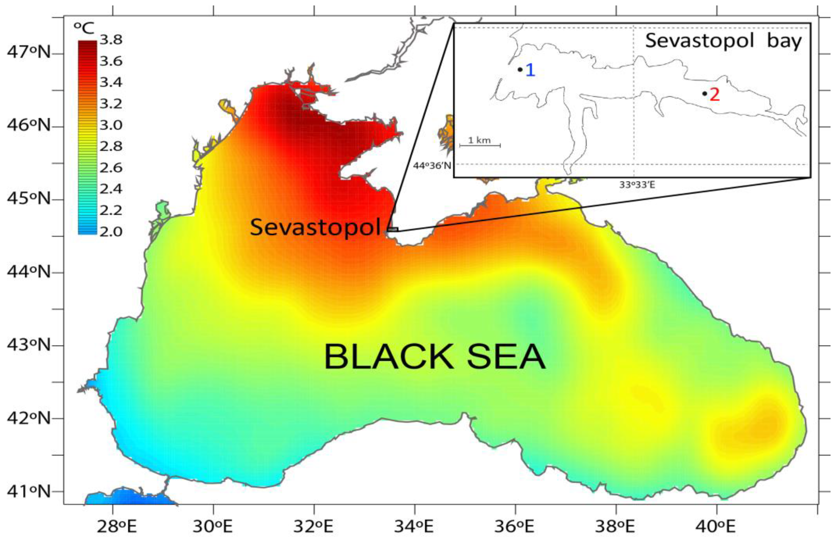
2.1. Area of Investigation

Sevastopol Bay is located in the northern part of the Black Sea at the southwestern tip of the Crimean Peninsula (Figure 1). It is about 7 km long and 1 km wide at its widest point, and it has an average depth of 12 m. It is a semi-enclosed estuarine-type bay having a restricted water exchange with the open sea because of its large length and the mole built at the entrance.

The salinity ranges within 14–17.5 ppt and is largely controlled by freshwater input from the Chernaya River that flows into the head of the bay [19]. The bay is suffering from a heavy anthropogenic pressure associated with discharges of industrial and domestic wastewaters as well as stormwater runoff. Based on the eutrophication E-TRIX-index assessments made in 2011–2012, the trophic level in the Sevastopol Bay was characterized as a transitional from medium to high [20]. Both pollution and trophic levels gradually decrease from the head of the bay to its mouth [21]. Being a port area, Sevastopol Bay is also heavily affected by maritime traffic, which contributes to invasions of alien species.

2.2. SST Data

SST in Sevastopol Bay is investigated based on a long-term series of continuous 6 h measurements from 1950 to 2014 provided by the Sevastopol Hydrometeorological Station. Additionally, the SST product from the OSTIA archive (Operational Sea Surface Temperature and Sea Ice Analysis) with a spatial resolution of 0.054° (about 5 km) was used to analyze the spatial distribution of the summer 2010 warm anomaly in the Black sea. The archive includes daily fields averaged using optimal interpolation and is based on satellite data from sensors AVHRR, AMSRE, AATSR, SEVERI and TMI, as well as on data received from drifting and moored buoys [22].

2.3. Sampling and Zooplankton Processing

The analysis of the mesozooplankton community is based on a long-term data set collected between 2003 and 2014 at two stations (Figure 1), one located in the mouth of Sevastopol Bay (station 1) and the other one in the middle of the bay (station 2). Throughout the entire period, sampling and samples processing were made according to the same methods, allowing a reliable assessment of seasonal and interannual changes.

Zooplankton samples were taken twice per month in the morning using a Juday plankton net (with a mouth area of 0.1 m² and a mesh size of 150 mm) from the whole water column: 10–0 m at station 1, and 9–0 m at station 2. Samples were fixed with formaldehyde solution (4% final conc.) and processed in the laboratory using the standard methodology for zooplankton. The sample was homogenized before taking aliquot. A calibrated 1 mL Stempel pipette was used for sub-sampling. Quantitative and qualitative processing was carried out in Bogorov’s chamber under a stereomicroscope. At least 2 aliquots were calculated for each sample. In the sub-sample(s), all crustaceans were counted until each of the three dominant species reached 100 individuals. The entire specimen was examined for rare species [23,24].

2.4. Data Analysis

2.4.1. SST Data

The monthly seasonal cycle of SST (or monthly mean climatology) was calculated based on observed mean monthly data averaged for each calendar month over the 30-year period from 1985 to 2014. The monthly SST anomalies were then calculated by subtracting the monthly seasonal cycle from the observed monthly means. In order to obtain the monthly mean climatology on a daily basis, the monthly climatology was interpolated from 12 calendar months to 365 calendar days using a spline interpolation.

To describe the summer 2010 MHW characteristics, we used the MHW definition from [25]: the mean daily SST exceeds a seasonally varying threshold (95th percentile) for at least 5 consecutive days; successive heatwaves with gaps of 2 days or less are considered part of the same event. The seasonally varying 95th percentile was calculated as monthly 95th percentile climatology for each calendar month over the period 1985–2014 and then interpolated to 365 calendar days using a spline interpolation.

2.4.2. Zooplankton

Based on the long-term observation dataset described in Section 2.3, seasonal and interannual variability in zooplankton abundance was analyzed at both stations for 12 species of crustacean zooplankton representing different ecological groups (warm-water, cold-water and eurythermal).

The seasonal variability of zooplankton species abundance was analyzed based on normalized average monthly values calculated as:

N_{i j}^{σ} = (\overset{ˉ}{N_{i j}} - \overset{ˉ}{\overset{ˉ}{N_{j}}}) / σ \overset{ˉ}{\overset{ˉ}{N_{j}}}

(1)

where

\overset{ˉ}{N_{i j}}

—average monthly values of the abundance for each i-th month and j-th species;

\overset{ˉ}{\overset{ˉ}{N_{j}}}

and σ

\overset{ˉ}{\overset{ˉ}{N_{j}}}

the average long-term value of the abundance and its standard deviation for the j-th species, respectively.

Interannual abundance variability was estimated as the deviation of the numbers of each zooplankton species (N_ij) from the corresponding average monthly values (for each i-th month and j-th species) according to:

δ N_{i j} = N_{i j} - \overset{ˉ}{N_{i j}}

(2)

Furthermore, the values of abundance anomalies relative to the annual variation (δN_ij) were averaged over the 2003 to 2014 (

\overset{ˉ}{δ N_{i j}}

), and the standard deviation σ(

\overset{ˉ}{δ N_{i j}}

) of the obtained time series were calculated. The average annual values of abundance anomalies relative to the annual variation normalized to this value (

{}_{δ}^{σ}{\bar{N}}

_ij) were used to characterize the interannual variability of particular zooplankton species and to assess the significance of differences in their abundance among years.

Hereafter, the normalized average annual values of abundance anomalies relative to the annual variation

{}_{δ}^{σ}{\bar{N}}

will be referred to as the indicator of interannual variability.

3. Results

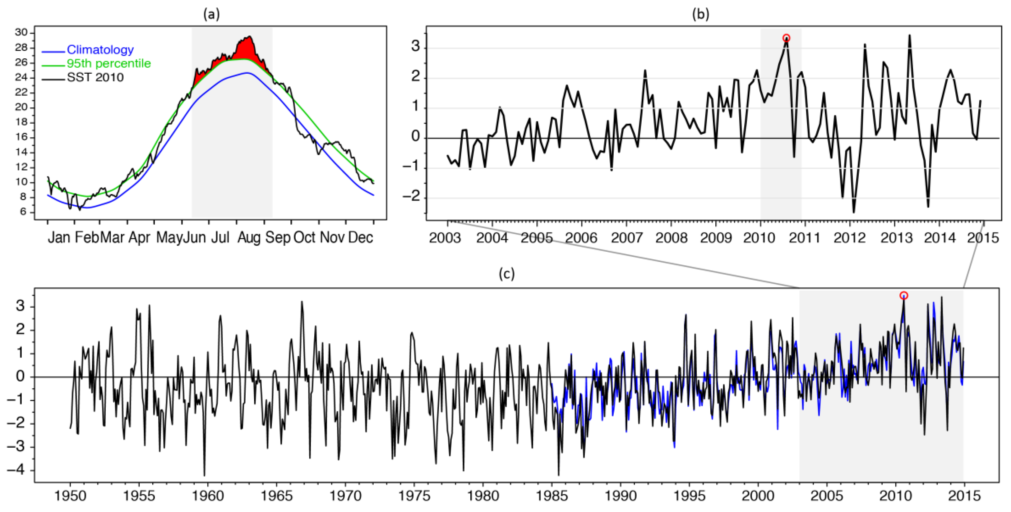
3.1. SST Variability and the Summer 2010 MHW

The SST of Sevastopol Bay has a marked seasonal cycle with a cold season from January to March and a warm season occurring form June to September (Figure 2a, blue line). The minimum and maximum are observed in February (6.6 °C) and August (24.8 °C), respectively. During the study period, SST shows a clear warming trend from 2003 to 2010, the latter year being the hottest one (Figure 2b). The month-to-month variability was rather low between 2003 and 2010. The period 2011–2014 exhibits stronger variability, which is associated in particular with two cold events (February 2012 and October 2013) when the monthly anomalies fell below −2 °C and the hottest event in May 2013 when the monthly anomaly reached 3.4 °C. The minimum and maximum are observed in February (6.6 °C) and August (24.8 °C), respectively.

During the study period (Figure 2b), SST shows a clear warming trend from 2003 to 2010, the latter year being the hottest one. The month-to-month variability was rather low between 2003 and 2010. The period 2011–2014 exhibits stronger variability, which is associated in particular with two cold events (February 2012 and October 2013) when the monthly anomalies fell below −2 °C and the hottest event in May 2013 when the monthly anomaly reached 3.4 °C. Figure 2c further evidences that the study period (2003–2014) corresponds to the warmest duodecad and 2010 is the warmest year since at least 1950 when began regular SST observations in Sevastopol Bay.

We now focus on the summer 2010 MHW event. Figure 2a shows that during almost all of 2010, the daily SST anomalies were above the climatological values. The summer MHW event starts on June 11th and ends on 9th September, lasting in total 3 months. The peak of the event was observed from 1 August to 19 August, when the daily SST anomalies exceeded 4 °C and reached 5 °C on 15 August. Figure 1 shows that in August 2010, abnormally high SSTs were recorded throughout the entire Black Sea area. The mean monthly anomalies ranged from about 2 °C in the Bosphorus region to almost 3.8 °C near the Dnieper-Bug Estuary in the northwestern shelf. Crimea’s southwestern coast was marked by extremely high values (more than 3 °C), which closely matched the in situ observations in Sevastopol Bay (Figure 2).

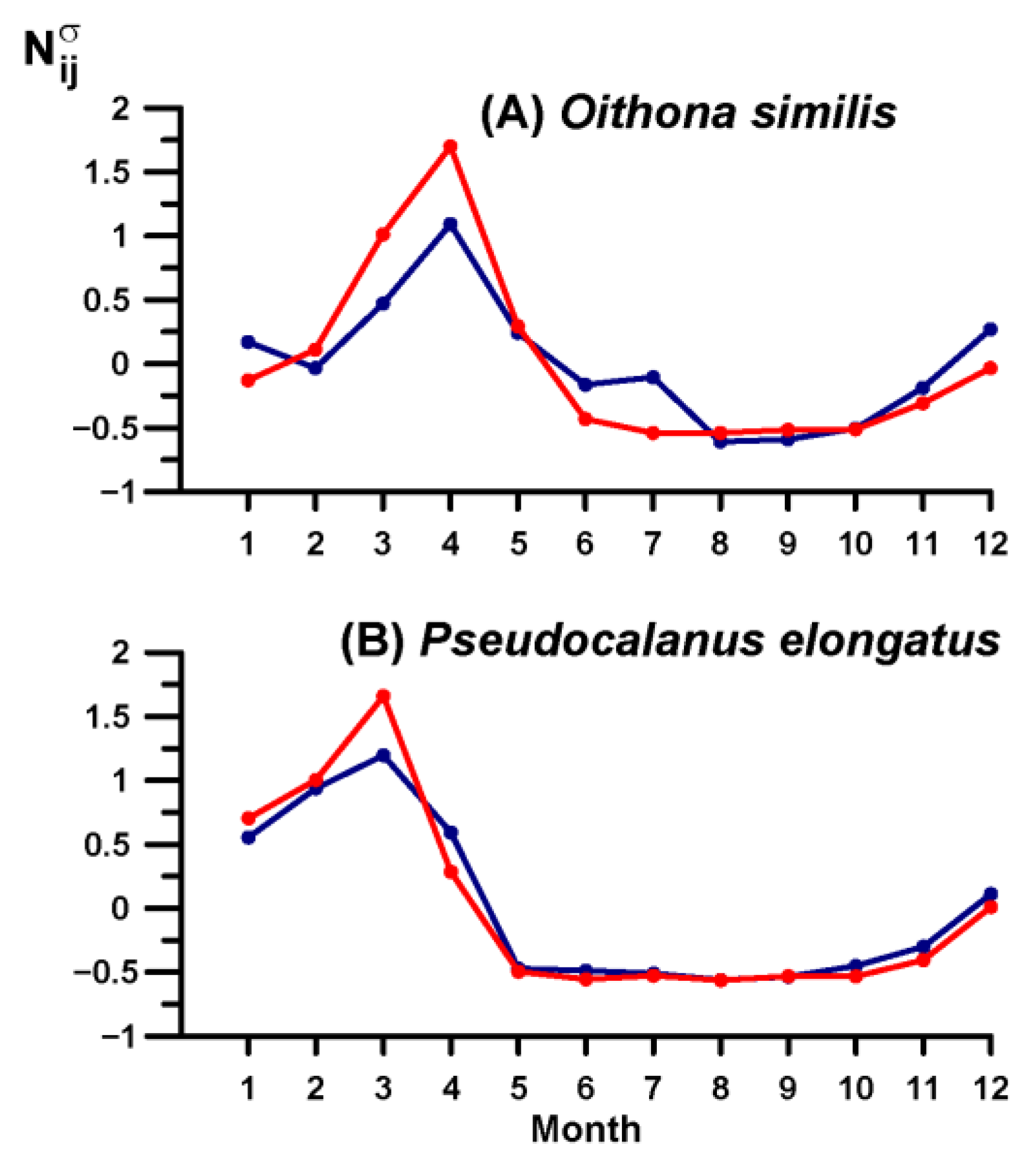
3.2. Species Composition and Ecological Groups of Zooplankton

During the study period, 12 species of crustaceans representing three different ecological groups (thermophilic, eurythermal and cold-water) were found in Sevastopol Bay. Table 1 summarizes the annual average abundance of each species. Copepods Acartia tonsa, Centropages ponticus, Oithona davisae and cladocerans Penilia avirostris, Pseudevadne tergestina, Evadne spinifera are representatives of a thermophilic assemblage. Among them, A. tonsa and O. davisae are non-indigenous species, which appeared in the Black Sea in 1970s and 2005, respectively. Pseudevadne tergestina and Evadne spinifera were not numerous and were not considered here.

The seasonal pattern dynamics of warm-water species are shown in Figure 3. All these species survived in the cold season in the Black Sea at a dormant stage. Most of them produced resting eggs in response to low temperatures, and O. davisae maintained in plankton at the stage of fertilized females. The populations of warm-water species began to grow rapidly in late May (at a temperature of 16–18 °C) and peaked in August–October (Figure 3A–C).

Such seasonal pattern was typical for all the above-mentioned species with the exception of C. ponticus (Figure 3D). The first peak of C. ponticus abundance occurred in June, which was followed by a slight decline in the hottest months of July and August. The more pronounced peak took place in September (Figure 3D). So, despite the fact that centropages is typically a warm-water species, it preferred temperatures not higher than 23 °C.

The eurythermal assemblage of crustaceans was represented by copepods A. clausi, P. parvus and cladocera P. polyphemoides. All these species are numerous in the Sevastopol Bay plankton community all year round. Seasonal pattern of A. clausi demonstrated two pronounced picks, in early spring (March) and autumn (September–November), respectively (Figure 4A). P. parvus peaked in November–December (Figure 4B). For both species, there was a summertime decline in abundance. (Figure 4A,B). P. polyphemoides showed strong picks only in May–June (Figure 4C).

Copepods P. elongatus, O. similis, C. euxinus belong to a cold-water assemblage. Two of them, P. elongatus and O. similis, are important components of the zooplankton of Sevastopol Bay in cold seasons. C. euxinus, an inhabitant of the open Black Sea, was found in small amounts in the bay, usually during winter. It was not taken under consideration in the present analysis. P. elongatus and O. similis were abundant in Sevastopol Bay during January–April and November–December, whereas in June–October, their density was the lowest (Figure 5A,B).

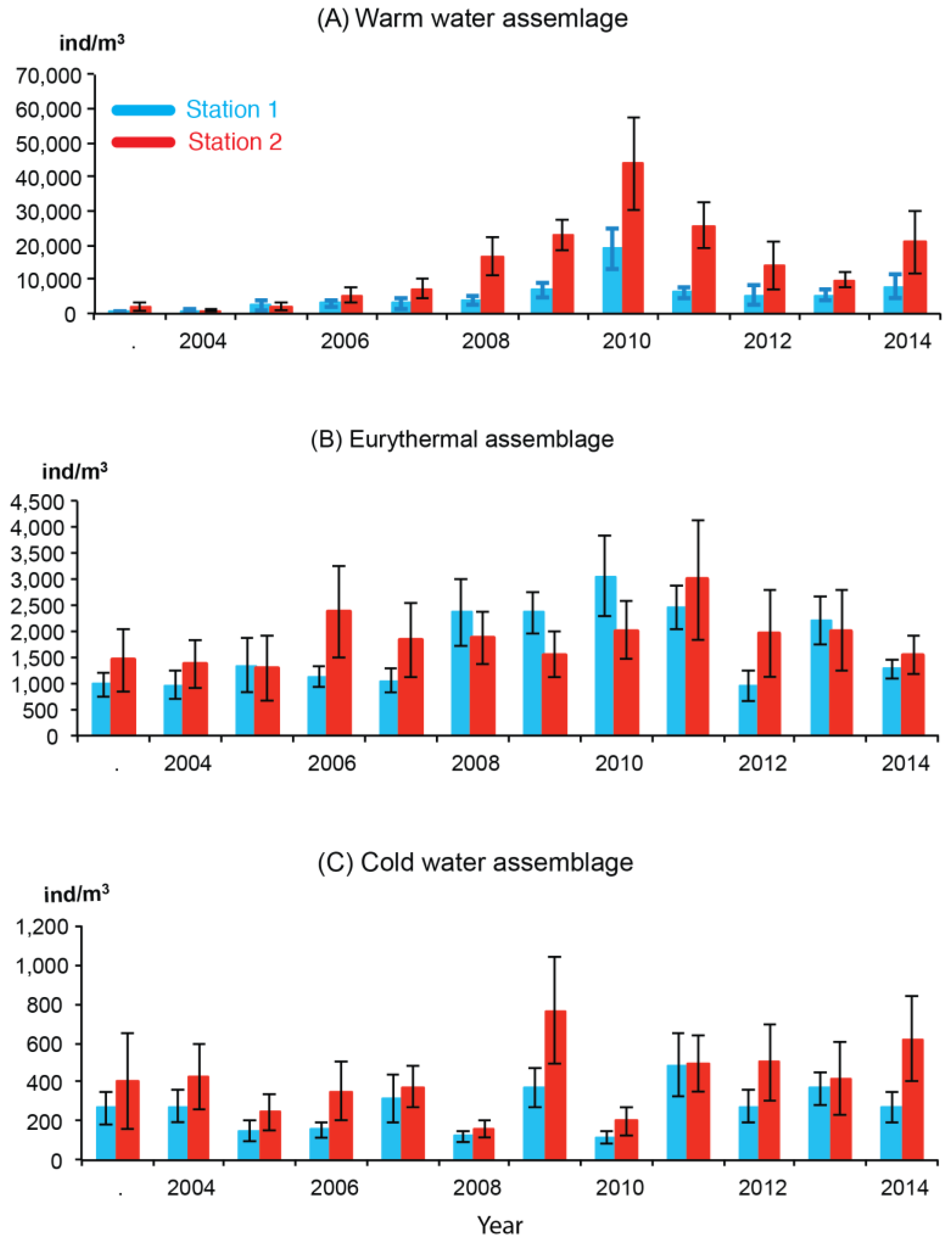
3.3. Interannual Variation in Abundance

For the study period 2003–2014, the maximum abundance of crustaceans was recorded in 2010: 22,000 ind. m⁻³ at the mouth of the bay (station 1) and 46,000 ind. m⁻³ in its middle (station 2), which is nearly three times the long-term average values for the whole period (about 7000 ind. m⁻³ and about 17,000 ind. m⁻³, respectively). At both stations, the crustaceans were numerically dominated by warm water species in 2010 (Table 1; Figure 6a). They amounted more than 19,000 ind. m⁻³ at station 1 and about 44,000 ± ind. m⁻³ at station 2 (85% and 95% of the total crustacean abundance, respectively). The warm-water assemblage prevailed not only among crustaceans but also in the mesozooplankton community as a whole, both by season (in the summer–autumn months) and by year (on average per year). Warm-water species abundance increased year after year from 2006 to 2010. This was attributable to the introduction and rapid growth of the O. davisae population, which is a new copepod species discovered in the Black Sea in 2005. Note also that a general positive trend in warm-water species abundance over 2003–2010 coincides with a strong warming SST trend in this period (Figure 2c).

The density of eurythermal and cold-water species varied slightly during the study period (Figure 6B,C). The eurythermal crustacean abundance ranged from 960 to 3057 ind. m⁻³ at station 1 and from 1292 to 2983 ind. m⁻³ at station 2, whereas the abundance of cold-water crustacean ranged from 119 to 487 ind. m⁻³ at station 1 and from 162 to 767 ind. m⁻³ at station 2. A minor rise in the abundance of eurythermal species was observed in 2010, notably at the mouth of the bay (Figure 6B). In the middle of the bay (station 2), the abundance of eurythermal species reached the highest values in 2011. On the contrary, the density of cold-water crustaceans was the lowest in 2010: 119 ind. m⁻³ at station 1 and 199 ind. m⁻³ at station 2 (Figure 6C).

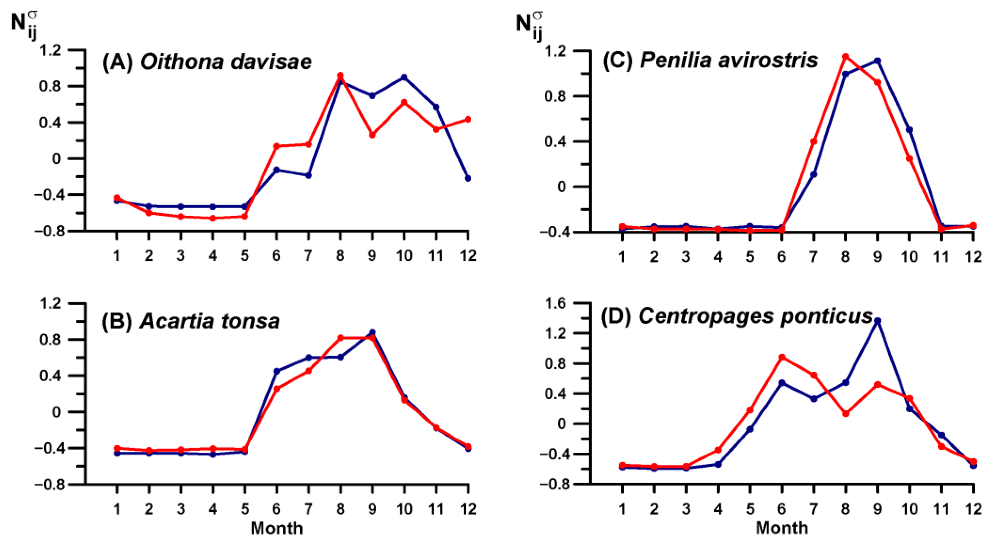
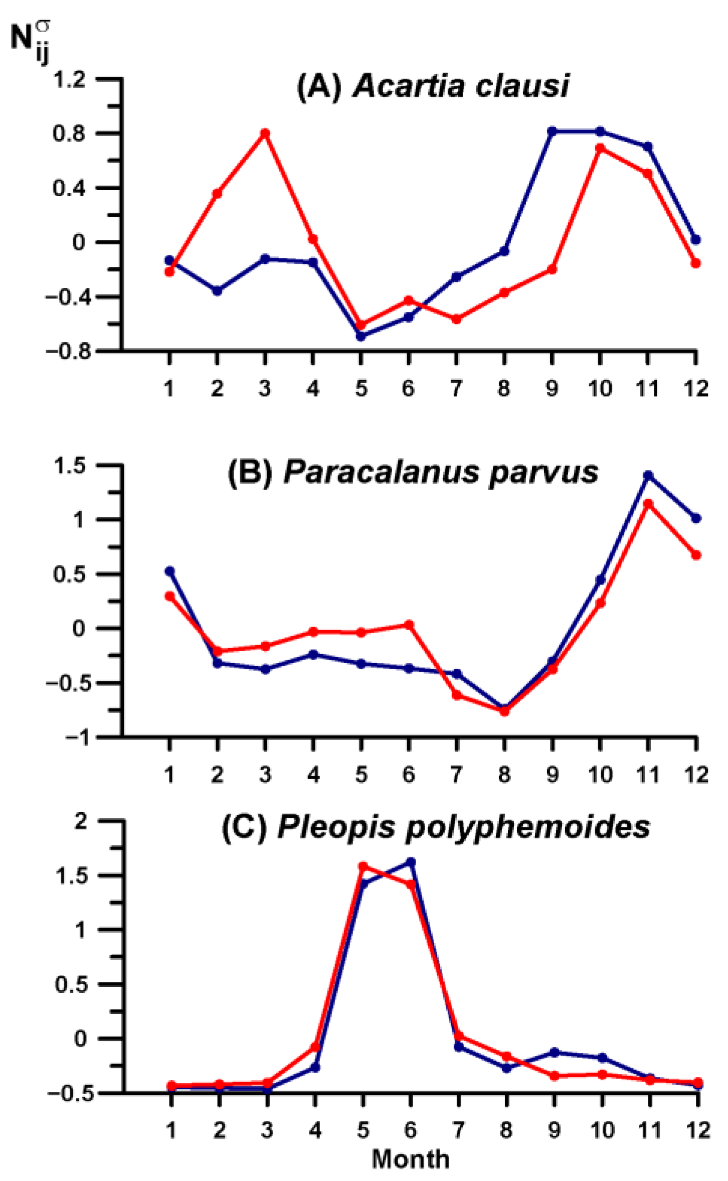
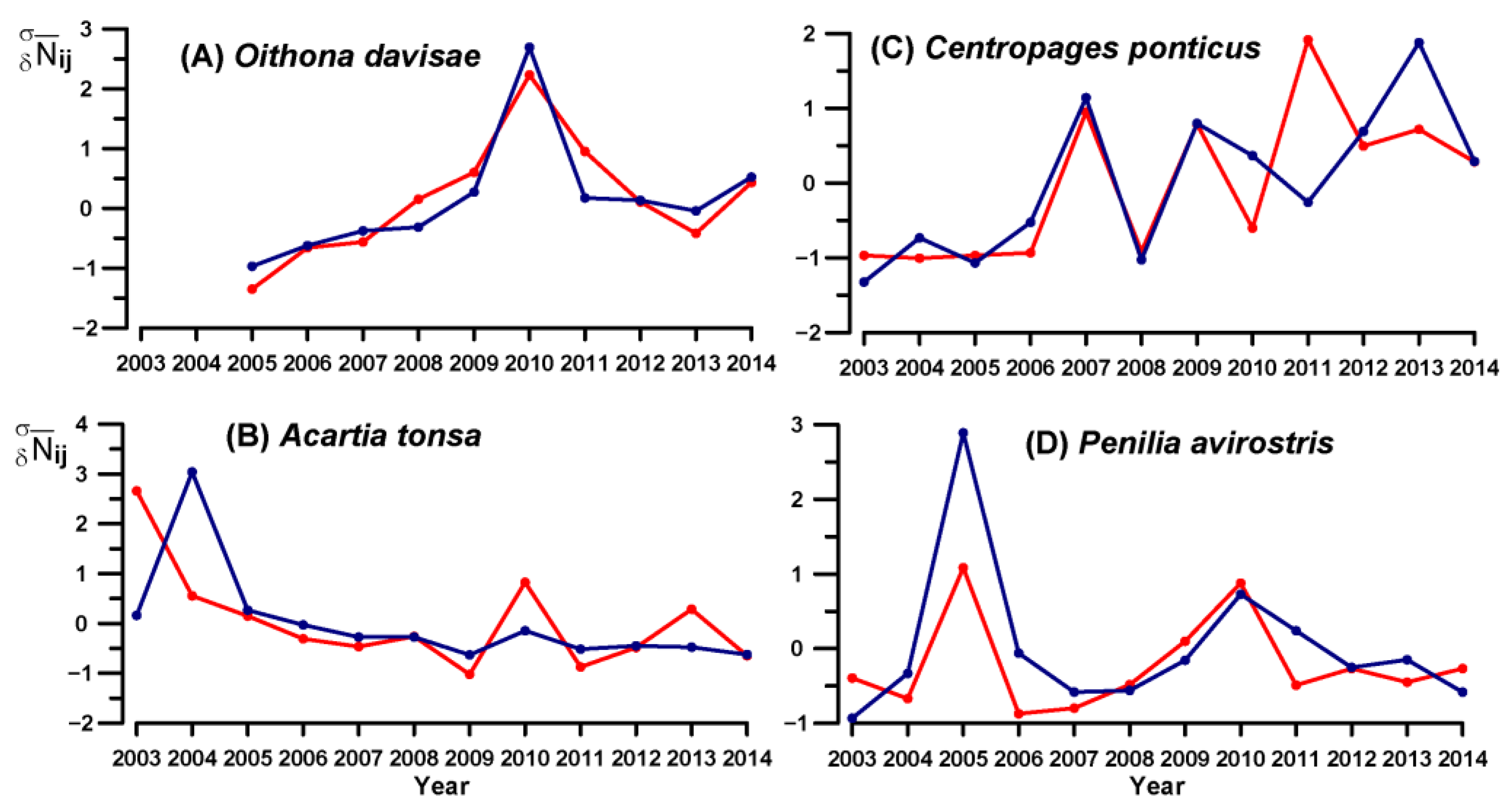
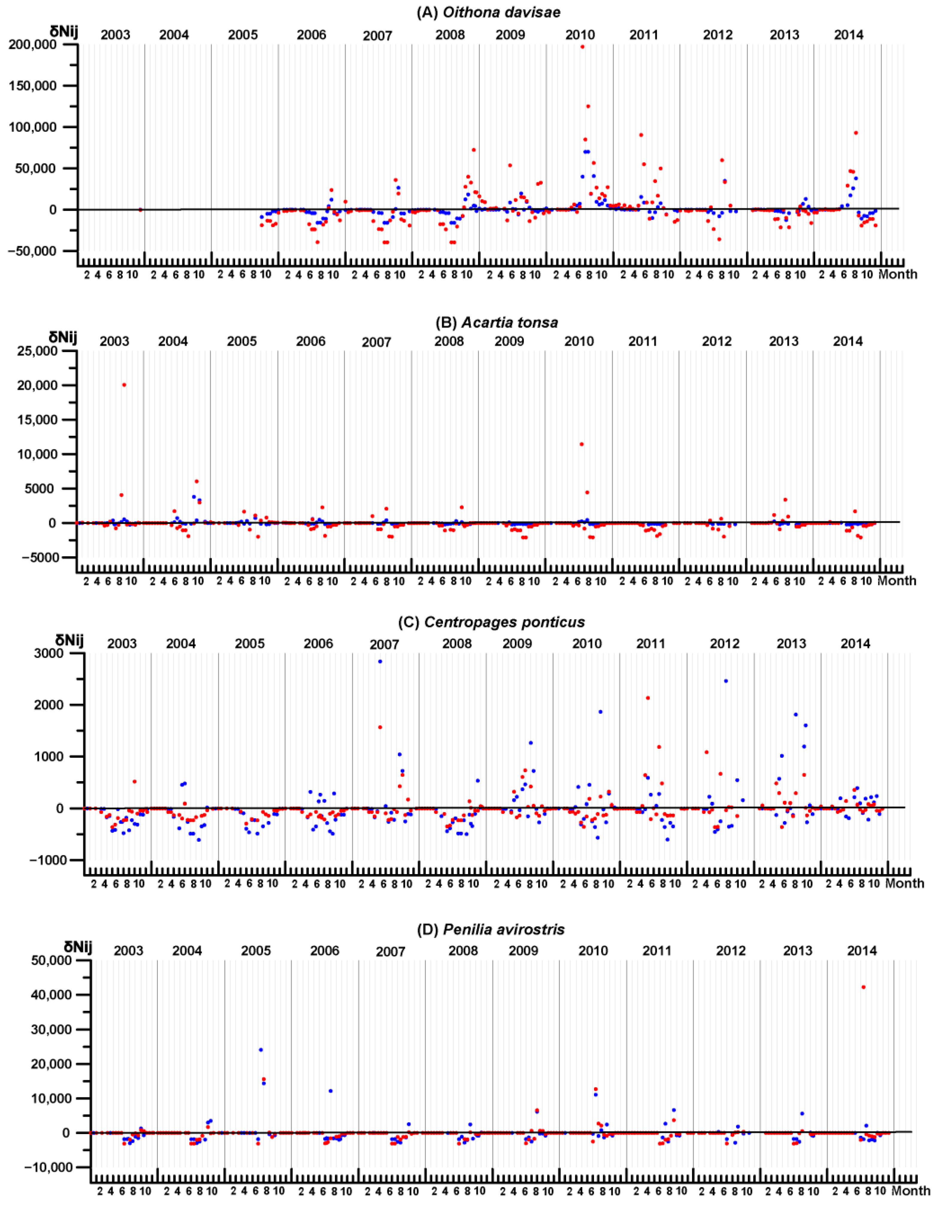
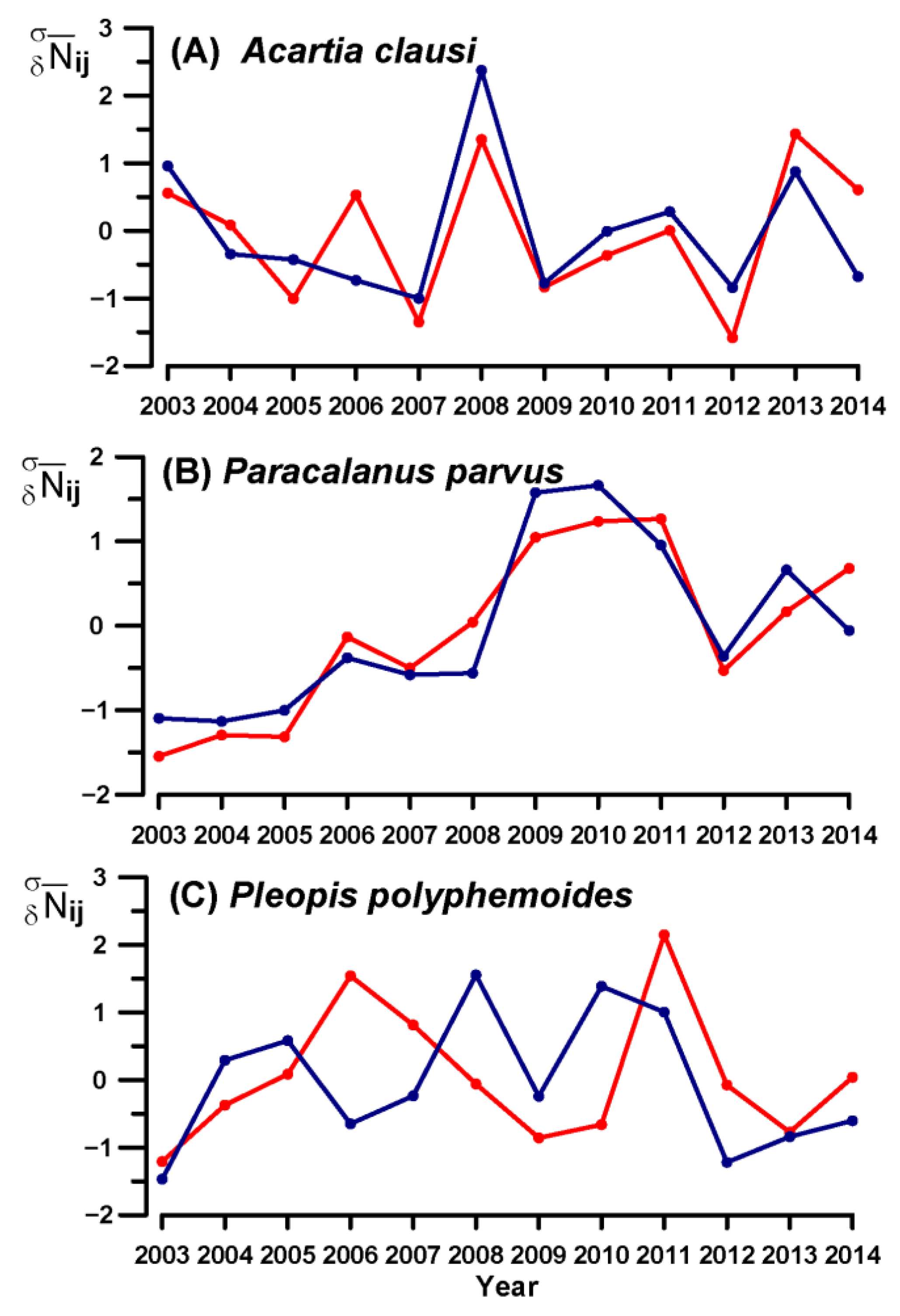
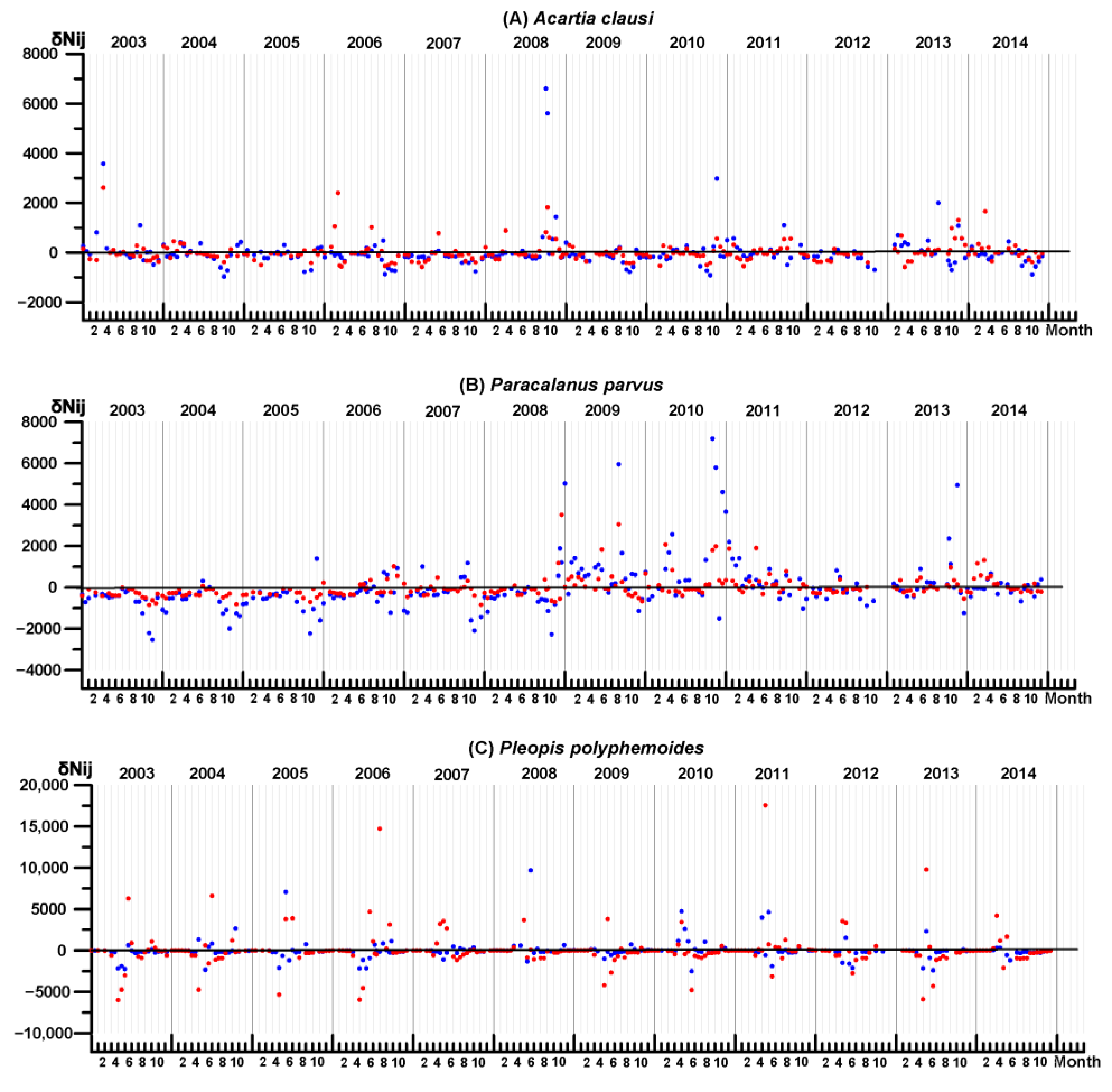
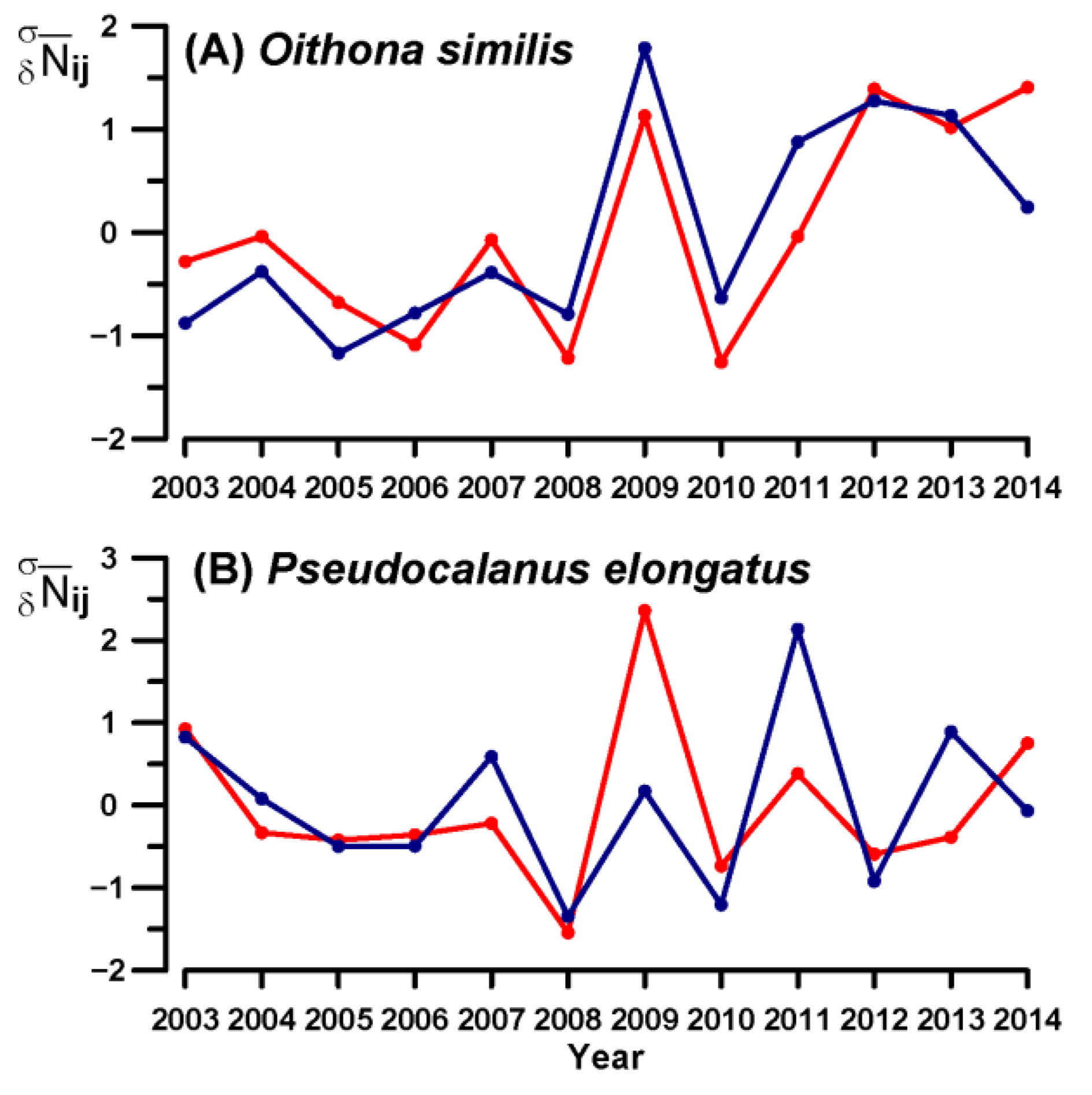
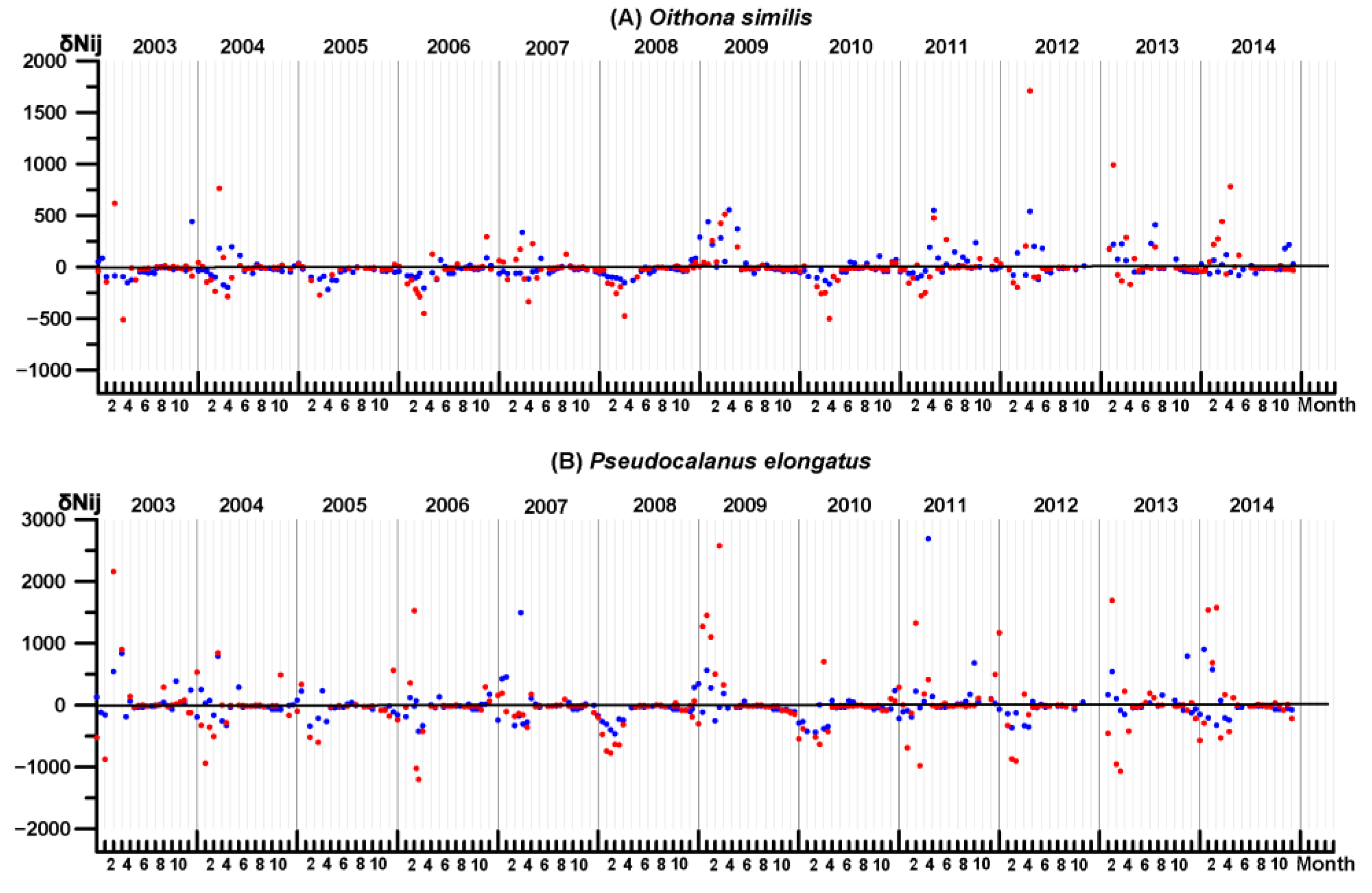
3.4. Key Species Variability

Warm-water assemblages of crustaceans in Sevastopol Bay were represented by four key species: O. davisae, A. tonsa, C. ponticus and P. avirostris. Non-indigenous copepod O. davisae was detected in the Black Sea at the end of 2005 and contributed the most to the total abundance of crustaceans in Sevastopol Bay during the following years. Since 2006, its abundance increased annually by about 1.5 times and reached 5770 ± 1763 ind. m⁻³ at station 1 and 22,069 ± 4345 ind. m⁻³ at station 2 in 2009 (Table 1). The population explosion occurred in 2010 (17,236 ± 5400 ind. m⁻³ at station 1 and 41,754 ± 12,337 ind. m⁻³ at station 2), and since 2011, species density stabilized near the values of 2009 (Table 1). At both stations, the indicator of interannual variability of abundance (

{}_{δ}^{σ}{\bar{N}}

) reached 3σ in 2010 (Figure 7A).

Positive anomalies in the abundance of O. davisae in Sevastopol Bay were observed throughout the entire breeding season of 2010 (Figure 8A). The largest abundance of O. davisae was recorded at both stations (86,000 ind. m⁻³ at station 1 and 145,000 ind. m⁻³ at station 2) in August 2010 during the peak of the summer MHW when the highest daily SST reached 29.6 °C. Moreover, O. davisae contributed hugely to the total abundance of crustaceans in August 2010: 78% at the mouth and 90% in the middle of the bay.

Another warm-water species A. tonsa was more abundant in 2003–2005, before the introduction of O. davisae (Figure 7B), showing the annual average density between 116 and 480 ind. m⁻³ at station 1 and between 599 and 1777 ind. m⁻³ at station 2. Since 2006, the density of A. tonsa decreased steadily, dropping to 52–99 (261–366) ind. m⁻³ at station 1 (station 2) in 2006–2008, and further to 3–38 (30–483) ind. m⁻³ at station 1 (station 2) in 2009 and 2011–2014 (Table 1). However, in 2010, the average annual abundance of A. tonsa increased sharply with respect to the previous years (up to 72 ± 35 ind. m⁻³ at station 1 and 883 ± 609 ind. m⁻³ at station 2). The maximum abundance was observed in July–August during the peak of the MHW (Figure 8B): 563 ind. m⁻³ and 12,000 ind. m⁻³ at the mouth and in the middle of the bay, respectively.

The warm-water species P. avirostris exhibited two pronounced peaks in its density in 2005 and 2010 (Table 1, Figure 7D). The peak of 2005 at the mouth of the bay (station 1) was the most significant and showed the indicator of interannual variability above 3σ. The average abundance in 2010 amounted to 1164 ind. m⁻³ ± 374 at station 1 and to 1202 ind. m⁻³ ± 749 at station 2. P. avirostris density reached the maximum in July–August (Figure 8D): the abundance was 7000–8000 ind. m⁻³ in July and 3000–4000 ind. m⁻³ in August (Table 1). The indicator of interannual variability reached 1σ for these peaks (Figure 7D).

Unlike the three warm-water species described above, the pattern of interannual fluctuations in C. ponticus abundance was more heterogenous, showing different behaviors at two stations (Figure 7C). The annual average density of C. ponticus reached its maximum in 2013 at station 1 (471 ± 159 ind. m⁻³) and 2011 at station 2 (284 ± 130 ind. m⁻³) (Table 1). Both stations did not experience a density peak in 2010 showing the values of 268 ± 109 ind. m⁻³ and 79 ± 28 ind. m⁻³ at station 1 and station 2, respectively. In August 2010, negative anomalies of C. ponticus abundance were observed at both stations (Figure 8D).

Eurythermal crustacean assemblages were represented by A. clausi, P. parvus and P. polyphemoides. The pattern of interannual variability of A. clausi showed a significant increase in population in 2008 and 2013 (Figure 9A) associated with seasonal picks in its abundance in spring and autumn (Figure 10A).

The annual average abundance of A. clausi ranged within 125 ± 35 ind. m⁻³ and 922 ± 408 ind. m⁻³ at station 1 and within 83 ± 17 ind. m⁻³ and 485 ± 117 ind. m⁻³ at station 2 (Table 1). In 2010, the abundance was close to the average value (362 ± 162 and 232 ± 62 ind. m⁻³ at stations 1 and 2, respectively). The annual average abundances of P. parvus increased at both stations in period 2009–2011 (Figure 9B), with the maximum density in 2010 (1830 ± 567 ind. m⁻³ at station 1 and 731 ± 192 ind. m⁻³ at station 2) (Table 1). The highest abundance of P. parvus occurred in November 2010 at the mouth of the bay (9100 ind. m⁻³). The abundance was also high in April–May and in October–December in 2010.

Positive anomalies of P. parvus were observed from January to May 2010 and from October 2010 to February 2011 (Figure 10B). The abundance of P. parvus was significantly higher at the mouth of the bay over the study period.

Unlike other species, the extremes of the interannual variability in the abundance of P. poliphemoides did not coincide at two stations (Figure 9C). At the mouth of the bay, the maximum of annual average density was in 2010 (865 ± 374 ind. m⁻³) followed by 2008 (799 ± 513 ind. m⁻³) and 2011 (795 ± 426 ind. m⁻³). In the middle of the bay, the most abundant year was 2011 (2027 ± 1086 ind. m⁻³), although 2010 was also abundant (1056 ± 511 ind. m⁻³) (Table 1). These interannual extremes were largely contributed by strong positive anomalies in abundance observed in May–June at both stations (Figure 10C).

The density of cold-water species P. elongatus and O. similis was low throughout the study period (Table 1). Their annual average abundance fluctuated from year to year, and the long-term variability of its anomalies had an irregular pattern (Figure 11A,B). A common feature of the long-term variability curves for both species was an increase in the density in 2009 and a decline in 2008 and 2010. (Figure 11A,B). Negative anomalies in the seasonal dynamics of P. elongatus and O. similis were observed from January to April in 2008 and 2010 (Figure 12A,B).

The annual average abundance of P. elongatus ranged between 55 ± 21 ind. m⁻³ and 352 ± 141 ind. m⁻³ at station 1 and 130 ± 40 ind. m⁻³ and 598 ± 228 ind. m⁻³ at station 2. The maximum seasonal abundance of P. elongatus occurred in February and March, the strongest peak being observed in March 2009 (about 4000 ind. m⁻³). The density of O. similis varied from 23 ± 9 ind. m⁻³ to 160 ± 46 ind. m⁻³ at station 1 and from 20 ± 7 ind. m⁻³ to 247 ± 151 ind. m⁻³ at station 2. The maximum seasonal abundance of O. similis was observed in February and April, the highest value of about 1500 ind. m⁻³ being found in April 2014.

4. Discussion

As a distinct signature of contemporary global warming, the MHWs are increasing in frequency, duration and magnitudes, posing a serious threat for the marine ecosystem. The Black Sea is an example of semi-closed sea experiencing a rapid warming, which is considered an amplified precursor of the changes to expect in the greater oceans [3]. Recent studies have shown that the frequency of MHW in the Black Sea has increased by a factor of five in the last two decades compared with the two previous decades [4].

In this study, we assessed the response of the zooplankton in Sevastopol Bay to the summer 2010 event, which was among the most persistent and intense MHW recorded in the Black Sea. In order to interpret the changes observed in 2010, the patterns of seasonal dynamics and interannual variability in the abundance of crustacean species were analyzed based on a dataset of zooplankton samples collected twice per month between 2003 and 2014.

The analysis of the SST in Sevastopol Bay showed that the study period was the warmest duodecad since at least 1950. Within this period, the SST showed a strong increasing trend between 2003 and 2010. 2010 was the warmest year since 1950 and exhibited positive SST anomalies almost all year round. The summer 2010 MHW starts at the beginning of June and lasts for 3 months, reaching the maximum amplitudes (daily SST anomaly > 4 °C) between the end of July and mid-August. Extreme positive SST anomalies in 2010 led to a sharp increase in the abundance of three warm-water species of crustaceans, namely O. davisae, A. tonsa and P. avirostris, and their share in the mesozooplankton community of Sevastopol Bay. An increase in the annual abundance in 2010 was also observed for two eurythermal species P. parvus and P. poliphemoides, although it is not related to the MHW event but can be rather explained by warm SST anomalies during the first part of the year. We now discuss in detail the response of each species to the MHV 2010 depending on unique peculiarities of its biology, seasonal dynamics and sensitivity to high temperature.

4.1. Warm-Water Assemblages

The largest contribution to the total abundance of crustaceans in 2010 was made by a non-indigenous species (NIS) of warm-water copepod Oithona davisae. This species was discovered in the Black Sea for the first time in October 2005 (it was initially misidentified as Oithona brevicornis) [26,27]. Its abundance rapidly increased, and already in 2006, Oithona davisae outnumbered other copepods in summer–autumn and on average per year [28]. A logarithmic acceleration phase such as a phase of NIS invasion pattern was observed in 2006–2008, when abundance raised sharply [29,30]. Afterwards, the growth was limited, and density remained at the same level as in 2009–2014, with the exception of 2010. In 2010, the abundance of O. davisae was extremely high with a maximum in July–August during the peak of the summer MHW 2010. A general positive trend in O. davisae abundance over 2003–2010 coincides with a strong warming SST trend in this period. We suggest that the increase in temperature during this period promoted the rapid growth in the population of O. davisae.

The other non-indigenous warm-water copepod A. tonsa appeared in the Black Sea in the 1970s [31,32]. It dominated the Sevastopol Bay in summer–autumn to 2006 before colonization of the bay by O. davisae. A considerable and statistically significant decline in A. tonsa abundance occurred from 2006 to 2014 due to competitive interactions between the two non-indigenous copepods [30]. It is worth noting that the negative effect of the non-indigenous O. davisae on populations of Acartia omori, Micosetelle norvegica and P. parvus have been also found in Tokyo Bay [33]. A sharp rise of the A. tonsa population in Sevastopol Bay was observed in July and August 2010 as a response to the MHW. The positive correlation of O. davisae and A. tonsa abundance with temperature was revealed in other areas of the world ocean [34,35,36].

At a seasonal scale, P. avirostris occurred in Sevastopol Bay in May–November and had one pronounced peak in August–September. The same seasonal dynamics was observed in the Mediterranean Vigo and Trieste regions, while in the subtropical highly productive waters of the Arabian Sea (Gulf of Oman), its population persisted all the year round. A regional link between the abundance of this species and temperature was also reflected in Gulf of Oman [37]. In Sevastopol Bay, the P. avirostris population was most abundant in 2005 and 2010 when strong positive SST anomalies were reported in August and September. A similar link between the average long-term abundance of P. avirostris and SST in August was reported for the coastal waters near Sevastopol [10].

Calanoid copepod C. ponticus is endemic to the Mediterranean and Black Sea [38,39]. It is a typical warm-water species that appears in plankton only during the warm season. However, unlike the warm-water species described above, O. davisae and A. tonsa, its peaks occurred in June and September at 22–23 °C. In July and August, when SST reached its maximum value, C. ponticus density declines. The annual average density of C. ponticus was relatively low in 2010 in Sevastopol Bay.

4.2. Eurythermal Assemblages

The native eurythermal Acartia clausi is one of the most common and numerous copepod in the World Ocean and also in the coastal area of the Black Sea [15,40,41,42]. In Sevastopol Bay, it was present year-round and reproduced throughout the year. According to long-term routine observations of zooplankton in the coastal area near Sevastopol in 1961–1969, a high abundance of A. clausi was observed in the years with negative temperature anomalies [10]. This is rather in line with our data: at the mouth of the bay, A. clausi exhibits the positive anomalies in its annual average density in the years when the SST anomalies in the bay was lower than 0.6 °C (2003, 2004, 2006, 2008, 2011 and 2013). In 2010, the annual population of A. clausi was close to its long-term average value, showing a seasonal peak in November, when the seasonal temperature drops. Thus, this eurythermal-type species did not show any response to the 2010 MHW.

Our results further suggested that the warm anomalies 2010 affected populations of eurythermal copepods P. parvus and P. polyphemoides. The highest average annual abundance of these species was reported in 2010 in Sevastopol Bay. The rise in P. parvus density was observed from February to June and in September-November 2010. The average annual abundance of P. polyphemoides in 2010 was higher than in other years, with positive abundance anomalies in spring and autumn, while in July and August, its abundance was low. Overall, the increase in annual abundance in 2010 of these eurythermal species can be explained by the rise of temperature in the first part of 2010, and it is not related to the summer MHW. Indeed, although both species occurred in the plankton of the bay all year round, their seasonal peaks occur in the spring and autumn and not in July–August when the 2010 MHW occurred. Interestingly, V.N. Grese with co-authors documented a significant summertime abundance of P. parvus in the coastal arear near Sevastopol in 1961–1969 [10]. The discrepancy in the seasonal patterns with their study could possibly be explained by the fact that the optimal temperature range for the P. parvus population development was reported between 10 and 20 °C, while over the study period, the late summer SST in Sevastopol Bay was near 26 °C, which led to a seasonal population decline.

4.3. Cold-Water Assemblage

Cold-water crustaceans were represented by copepods P. elongatus and O. similis. P. elongatus is common in the temperate eastern North Atlantic Ocean, including the Black Sea and some localities in Mediterranean Sea [43,44]. O. similis is cosmopolitan, distributed from tropical to polar waters [36,45]. In the summer, both species stay in the open Black Sea under a thermocline and appear in the surface waters and coastal areas in the cold season. In Sevastopol Bay, these copepods reached their greatest abundance in the first half of the year and were not found in summer. The year 2010 was one of the years characterized by the lowest annual average abundance of the cold-water species within the study period.

4.4. Concluding Remarks

Among all considered species, the most pronounced response to the summer 2010 MHW was observed in the population of non-native warm-water copepods O. davisae and A. tonsa at both seasonal and interannual scales. These species showed the ability of rapid population growth with rising temperatures. A large number of previous laboratory studies have indicated that increasing temperatures accelerate the development times of eggs and larval stages (nauplii and copepodids) of copepods [46,47]. Apparently, the extreme temperature in 2010 led to a reduction in the generation time of the warm-water species O. davisae and A. tonsa, resulting in a sharp increase in their abundance.

These NIS have a number of competitive advantages over native species. Their specific biological features ensured its rapid spread across the world ocean, establishment in new habitats, and successful competition with native species [30,48]. Non-native species also exhibit great flexibility as an adaptive response to environmental changes, especially in the case of climate warming.

The current climate changes significantly reduce the resistance of marine ecosystems to disturbance effects, which greatly facilitates the introduction of alien species into new ecosystems, especially into coastal areas [49]. The number of alien species and their abundance has increased in the Black Sea in recent decades. In addition to the described above A. tonsa and O. davisae, a new non-indigenous copepod P. marinus was reported in Sevastopol Bay in September 2016 [16,50]. All these new species are members of the warm-water mesozooplankton assemblage. Observations in other estuaries have also indicated that non-indigenous zooplankton species usually prevail in summer and autumn [34,36,50,51].

Studies of the climate warming impact on the marine ecosystems may be facilitated by the description of the indicator species. Following Reed Noss, the indicator should be (1) sensitive enough to warn of changes in a timely manner; (2) distributed over a wide geographic area or otherwise widely applicable; and (3) able to provide continuous assessment over a wide range of stresses [52]. Our results suggest that future warming may lead to an increase in O. davisae dominance in the mesozooplankton community of the Black Sea coastal area and that among crustaceans observed in this study, this species can be considered as an indicator of the environmental conditions associated with the warming of the Black Sea and the Mediterranean basin as a whole.

Author Contributions

Conceptualization, A.G. and K.G.; validation, A.G., K.S. and V.B., formal analysis, A.G., K.G., O.K. and V.B.; investigation, A.G., O.G., E.S. and T.L.; data curation, A.G., O.K.; writing—original draft preparation, A.G., K.G., O.K. and K.S.; writing—review and editing, A.G., K.G., O.K., T.L. and K.S.; supervision, A.G.; project administration, A.G. and O.K.; funding acquisition, A.G. and K.S. All authors have read and agreed to the published version of the manuscript.

Funding

The research was conducted in the frame of the Russian state assignments of Institute of Biology of the Southern Seas No. 121040600178-6; No. 121030100028-0 and of Marine Hydrophysical Institute FNNN-2021-0002 and the National Science Program “Environmental Protection and Reduction of Risks of Adverse Events and Natural Disasters”, approved by the Resolution of the Council of Ministers No. 577/17.08.2018 and supported by the Ministry of Education and Science (MES) of Bulgaria (Agreement No. Д01-279/03.12.2021).

Institutional Review Board Statement

Not applicable.

Informed Consent Statement

Not applicable.

Data Availability Statement

Not applicable.

Conflicts of Interest

The authors declare no conflict of interest.

References

Oliver, E.C.J.; Donat, M.G.; Burrows, M.T. Longer and more frequent marine heatwaves over the past century. Nat. Commun. 2018, 9, 1324. [Google Scholar] [CrossRef] [PubMed] [Green Version]
Pörtner, H.O.; Roberts, D.C.; Masson-Delmotte, V.; Zhai, P.; Tignor, M.; Poloczanska, E. Summary for policymakers. In IPCC Special Report on the Ocean and Cryosphere in a Changing Climate; IPCC: Geneva, Switzerland, 2019. [Google Scholar]
Stanev, E.V.; Peneva, E.; Chtirkova, B. Climate Change and Regional Ocean Water Mass Disappearance: Case of the Black Sea. J. Geophys. Res. Ocean. 2019, 124, 4803–4819. [Google Scholar] [CrossRef]
Mohamed, B.; Ibrahim, O.; Nagy, H. Sea Surface Temperature Variability and Marine Heatwaves in the Black Sea. Remote Sens. 2022, 14, 2383. [Google Scholar] [CrossRef]
Barriopedro, D.; Fischer, E.M.; Luterbacher, J.; Trigo, R.M.; García-Herrera, R. The Hot Summer of 2010: Redrawing the Temperature Record Map of Europe. Science 2011, 332, 220–224. [Google Scholar] [CrossRef] [PubMed] [Green Version]
Soulié, T.; Vidussi, F.; Mas, S.; Mostajir, B. Functional Stability of a Coastal Mediterranean Plankton Community During an Experimental Marine Heatwave. Front. Mar. Sci. 2022, 9, 831496. [Google Scholar] [CrossRef]
Richardson, A.J. In hot water: Zooplankton and climate change. ICES J. Mar. Sci. 2008, 65, 279–295. [Google Scholar] [CrossRef] [Green Version]
Maskas, D.L.; Beaugrand, G. Comparisons of zooplankton time series. J. Mar. Syst. 2010, 79, 286–304. [Google Scholar] [CrossRef]
Sazhina, L.T. Fertility of the mass pelagic copepoda in the Black Sea. Zool. Zhurnal 1971, 50, 586–588. (In Russian) [Google Scholar]
Greze, V.N.; Baldina, E.P.; Bileva, O.K. Dynamics of the abundance and production of the principal components of Zooplankton in the Neritic Zone of the Black Sea. Mar. Biol. 1971, 24, 12–49. (In Russian) [Google Scholar]
Evans, R.; Lea, M.-A.; Hindell, M.A.; Swadling, K.M. Significant shifts in coastal zooplankton populations through the 2015/16 Tasman Sea marine heatwave. Estuar. Coast. Shelf Sci. 2020, 235, 106538. [Google Scholar] [CrossRef]
McKinstry, C.A.E.; Campbell, R.W.; Holderied, K. Influence of the 2014–2016 marine heatwave on seasonal zooplankton community structure and abundance in the lower Cook Inlet, Alaska. Deep. Sea Res. Part II Top. Stud. Oceanogr. 2022, 195, 105012. [Google Scholar] [CrossRef]
Zaika, V.E. Marine biodiversity of the Black Sea and Eastern Mediterranean. Ecol. Sea 2000, 51, 59–62. (in Russian). [Google Scholar]
Benedetti, F.; Ayata, S.D.; Irisson, J.O.; Adloff, F.; Guilhaumon, F. Climate change may have minor impact on zooplankton functional diversity in the Mediterranean Sea. Divers. Distrib. 2019, 25, 568–581. [Google Scholar] [CrossRef]
Gubanova, A.D.; Altukhov, D.A.; Stefanova, K.; Arashkevich, E.G.; Kamburska, L.; Prusova, I.Y.; Svetlichny, L.S.; Timofte, F.; Uysal, Z. Species composition of Black Sea marine planktonic copepods. J. Mar. Syst. 2014, 135, 44–52. [Google Scholar] [CrossRef]
Gubanova, A.; Drapun, I.; Garbazey, O.; Krivenko, O.; Vodiasova, E. Pseudodiaptomus marinus Sato, 1913 in the Black Sea: Morphology, genetic analysis, and variability in seasonal and interannual abundance. PeerJ 2020, 8, e10153. [Google Scholar] [CrossRef]
Greze, V.N. Zooplankton. In Basics of Biological Productivity of the Black Sea; Greze, V.N., Ed.; Naukova Dumka: Kiev, Ukraine, 1979; pp. 143–164. (In Russian) [Google Scholar]
Finenko, Z. Biodiversity and Bioproductivity. In The Black Sea Environment. The Handbook of Environmental Chemistry; Water Pollution; Part, Q., Kostianoy, A.G., Kosarev, A.N., Eds.; Springer: Berlin/Heidelberg, Germany, 2008; Volume 5, pp. 351–374. [Google Scholar]
Garmashov, A. Hydrological characteristics of Sevastopol Bay. Int. Multidiscip. Sci. Geo Conf. SGEM 2019, 19, 247–252. [Google Scholar] [CrossRef]
Gubanov, V.I.; Gubanova, A.D.; Rodionova, N.Y. Diagnosis of water trophicity in the Sevastopol bay and its offshore. In Current issues in aquaculture: In Proceedings of the International Scientific Conference, Rostov-on-Don, Russia, 28 September–2 October 2015; pp. 64–67.
Litvinyuk, D.; Mukhanov, V.; Evstigneev, V. The Black Sea Zooplankton Mortality, Decomposition, and Sedimentation Measurements Using Vital Dye and Short-Term Sediment Traps. J. Mar. Sci. Eng. 2022, 10, 1031. [Google Scholar] [CrossRef]
Donlon, C.J.; Martin, M.; Stark, J.; Roberts-Jones, J.; Fielder, E.; Wimmer, W. The Operational Sea Surface Temperature and Sea Ice Analysis (OSTIA) system. Remote Sens. Environ. 2012, 116, 140–158. [Google Scholar] [CrossRef]
Postel, L.; Fock, H.; Hagen, W. Biomass and abundance. In ICES Zooplankton Methodology Manual; Harris, R.P., Wiebe, P.H., Lenz, J., Skjoldal, H.R., Huntley, M., Eds.; Academic Press: London, UK, 2000; pp. 83–174. [Google Scholar]
Aleksandrov, B.; Arashkevich, E.; Gubanova, A.; Korshenko, A. Black Sea monitoring guidelines mesozooplankton. Publ. EMBLAS Proj. BSC. 2014. Available online: http://www.blacksea-commission.org/Downloads/Mesozooplankton_Manual_2015_ISBN%20%20978-617-7953-33-2.pdf (accessed on 15 October 2020).
Hobday, A.J.; Alexander, L.V.; Perkins, S.E.; Smale, D.A.; Straub, S.C.; Oliver, E.C.J.; Benthuysen, J.A.; Burrows, M.T.; Donat, M.G.; Feng, M.; et al. A hierarchical approach to defining marine heatwaves. Prog. Oceanogr. 2016, 141, 227–238. [Google Scholar] [CrossRef] [Green Version]
Gubanova, A.; Altukhov, D. Establishment of Oithona brevicornis Giesbrecht, 1892 (Copepoda: Cyclopoida) in the Black Sea. Aquat. Invasions 2007, 2, 407–410. Available online: http://www.aquaticinvasions.net/2007/index4.html (accessed on 15 May 2007). [CrossRef]
Temnykh, A.; Nishida, S. New record of copepod Oithona davisae Ferrari and Orsi in the Black Sea with notes on the identity of Oithona brevicornis. Aquat. Invasions 2012, 7, 425–431. [Google Scholar] [CrossRef]
Altukhov, D.; Gubanova, A.; Mukhanov, V. New invasive copepod Oithona davisae Ferrari and Orsi, 1984: Seasonal dynamics in Sevastopol Bay and expansion along the Black Sea coasts. Mar. Ecol. 2014, 35, 28–34. [Google Scholar] [CrossRef]
Odum, E. Fundamentals of Ecology; Saunders, W.B., Ed.; Saunders: Philadelphia, PA, USA; Moscow, Russia, 1975. [Google Scholar]
Gubanova, A.D.; Garbazey, O.A.; Popova, E.V.; Altukhov, D.A.; Mukhanov, V.S. Oithona davisae: Naturalization in the Black Sea, interannual and Seasonal dynamics, and effect on the structure of the planktonic copepod community. Oceanology 2019, 59, 912–919. [Google Scholar] [CrossRef]
Belmonte, G.; Mazzocchi, M.G.; Prusova, I.Y.; Shadrin, N.V. Acartia tonsa: A species new for the Black Sea fauna. Hydrobiologiya 1994, 292, 9–15. [Google Scholar] [CrossRef]
Gubanova, A.D. Occurrence of Acartia tonsa Dana in the Black Sea. Was it introduced from the Metiterranean? Mediterr. Mar. Sci. 2000, 1, 105–109. [Google Scholar] [CrossRef]
Itoh, H.; Nishida, S. Spatiotemporal distribution of planktonic copepod communities in Tokyo Bay where Oithona davisae ferrari and orsi dominated in mid-1980s. J. Nat. Hist. 2015, 49, 2759–2782. [Google Scholar] [CrossRef]
Uriarte, I.; Villate, F.; Iriarte, A. Zooplankton recolonization of the inner estuary of Bilbao: Influence of pollution abatement, climate and non-indigenous species. J. Plankton Res. 2016, 38, 718–731. [Google Scholar] [CrossRef] [Green Version]
Kimmel, D.G.; Roman, M.R. Long-term trends in mesozooplankton abundance in Chesapeake Bay, USA: Influence of freshwater input. Mar. Ecol. Prog. Ser. 2004, 267, 71–83. [Google Scholar] [CrossRef]
Besiktepe, S.; Kurt, T.T.; Gubanova, A. Mesozooplankton composition and distribution in Izmir Bay, Aegean Sea: With special emphasis on copepods. Reg. Stud. Mar. Sci. 2022, 55, 102567. [Google Scholar] [CrossRef]
Piontkovski, S.A.; Fonda-Umani, S.; De Olazabal, A.; Gubanova, A.D. Penilia avirostris: Regional and Global Patterns of Seasonal Cycles. Int. J. Ocean. Oceanogr. 2012, 6, 9–25. [Google Scholar]
Sazhina, L.I.; Kovalev, A.V. About the synonymy of the Black Sea copepods. Zool. J. 1971, 50, 1099–1101. (In Russian) [Google Scholar]
Papantoniou, G.; Danielidis, D.B.; Spyropoulou, A.; Fragopoulu, N. Spatial and temporal variability of small-sized copepod assemblages in a shallow semi-enclosed embayment (Kalloni Gulf, NE Mediterranean Sea). J. Mar. Biolog. Assoc. UK 2015, 95, 349–360. [Google Scholar] [CrossRef]
Azeiteiro, U.M.; Marques, S.C.; Vieira, L.M.R.; Pastorinho, M.R.D.; Ré, P.A.B.; Pereira, M.J.; Morgado, F.M.R. Dynamics of the Acartia genus (Calanoida: Copepoda) in a temperate shallow estuary (the Mondego estuary) on the western coast of Portugal. Acta Adriat. 2005, 46, 7–20. [Google Scholar]
Jeffries, H.P. Succession of two Acartia species in estuaries. Limnol. Oceanogr. 1962, 7, 354–364. [Google Scholar] [CrossRef]
Lee, W.Y.; McAlice, B.J. Seasonal succession and breeding cycles of three species of Acartia (Copepoda: Calanoida) in a Marine estuary. Estuaries 1979, 2, 228–235. [Google Scholar] [CrossRef]
Frost, B.W. A taxonomy of the marine calanoid copepod genus Pseudocalanus. Can. J. Zool. 1989, 67, 525–551. [Google Scholar] [CrossRef]
Razouls, C.; de Bovée, F.; Kouwenberg, J.; Desreumaux, N. Diversity and Geographic Distribution of Marine Planktonic Copepods, 2005–2022. Available online: http://copepodes.obs-banyuls.fr/en (accessed on 18 November 2022).
Nishida, S. Taxonomy and distribution of the family Oithonidae (Copepoda, Cyclopoida) in the Pacific and Indian oceans. Bull. Ocean Res. Inst. Univ. Tokyo 1985, 20, 1–167. [Google Scholar]
Vijverberg, J. Effect of temperature in laboratory studies on development and growth of Cladocera and Copepoda from Tjeukemeer, The Netherlands. Freshw. Biol. 1980, 10, 317–340. [Google Scholar] [CrossRef]
Huber, V.; Adrian, R.; Gerten, D. A matter of timing: Heat wave impact on crustacean zooplankton. Fresh Water Biol. 2010, 55, 1769–1779. [Google Scholar] [CrossRef]
Cornils, A.; Wend-Heckmann, B. First report of the planktonic copepod Oithona davisae in the northern Wadden Sea (North Sea): Evidence for recent invasion? Helgol. Mar. Res. 2015, 69, 243–248. [Google Scholar] [CrossRef] [Green Version]
Rice, E.; Dam, H.G.; Stewart, G. Impact of climate change on estuarine zooplankton: Surface water warming in long Island sound is associated with changes in copepod size and community structure. Estuaries Coasts 2015, 38, 13–23. [Google Scholar] [CrossRef]
Uttieri, M.; Aguzzi, L.; Aiese Cigliano, R.; Amato, A.; Bojanić, N.; Brunetta, M.; Camatti, E.; Carotenuto, Y.; Damjanović, T.; Delpy, F.; et al. WGEUROBUS—Working Group ‘‘Towards a European Observatory of the non-indigenous calanoid copepod Pseudodiaptomus marinus”. Biol. Invasions 2020, 22, 885–906. [Google Scholar] [CrossRef]
Bollens, S.M.; Breckenridge, J.; Cordell, J.R.; Simenstad, C.; Kalata, O. Zooplankton of tidal marsh channels in relation to environmental variables in the upper San Francisco Estuary). Aquat. Biol. 2014, 21, 205–219. [Google Scholar] [CrossRef] [Green Version]
Noss, R.F. Indicators for Monitoring Biodiversity: A Hierarchical Approach. Conserv. Biol. 1990, 4, 355–364. [Google Scholar] [CrossRef]

Figure 1. Sampling stations in Sevastopol Bay and spatial pattern of the monthly average sea surface temperature (SST, °C) anomalies in the Black Sea in August 2010 with respect to the 1985–2014 monthly climatology.

Figure 2. SST series in Sevastopol Bay (°C): (a) The climatology (blue), 95th percentile marine heat wave (MHW) threshold (green) and time series (black) for 2010. The red filled area indicates the period of time associated with the MHW; (b) Monthly averaged anomalies over the study period 2003–2014 with respect to the 1985–2014 monthly climatology as recorded by in situ observations; (c) As in (b) but over the period 1950–2014. Black and blue lines in (c) show the in situ and satellite observations, respectively.

Figure 3. The patterns of seasonal dynamics of warm-water crustaceans in Sevastopol Bay at station 1 (blue) and station 2 (red) presented as normalized average monthly values (see details of the method in Section 2.4): (A)—Oithona davisae; (B)—Acartia tonsa; (C)—Centropages ponticus; (D)—Penilia avirostris.

Figure 4. The patterns of seasonal dynamics of eurythermalcrustaceansin Sevastopol Bay at station 1 (blue) and station 2 (red) presented as normalized average monthly values (see details of the method in Section 2.4): (A)—Acartia clausi; (B)—Paracalanus parvus; (C)—Pleopis polyphemoides.

Figure 5. The patterns of seasonal dynamics of cold-water crustaceans in Sevastopol Bay at station 1 (blue) and station 2 (red) presented as normalized average monthly values (see details of the method in Section 2.4): (A)—Oithona similis; (B)—Pseudocalanus elongatus.

Figure 6. Interannual variability of annual average abundance of the: (A)—warm-water crustacean assemblage, (B)—euthermal crustacean assemblage; (C)—cold-water crustacean assemblage in Sevastopol Bay at station 1 (blue bars) and station 2 (red bars).

Figure 7. Pattern of interannual variability of abundance of the warm-water crustaceans in Sevastopol Bay at station 1 (blue) and station 2 (red) presented as normalized annual anomalies (see details of the method in Section 2.4): (A)—Oithona davisae; (B)—Acartia tonsa; (C)—Centropages ponticus; (D)—Penilia avirostris.

Figure 8. Long-term fluctuations in anomalies of warm-water crustaceans abundance relative to the annual variation (see details of the method in Section 2.4) in Sevastopol Bay at station 1 (blue) and station 2 (red): (A)—Oithona davisae; (B)—Acartia tonsa; (C)—Centropages ponticus; (D)—Penilia avirostris.

Figure 9. Pattern of interannual variability of abundance of eurythermal crustaceans in Sevastopol Bay at station 1 (blue) and station 2 (red) presented as normalized annual anomalies (see details of the method in Section 2.4): (A)—Acartia clausi; (B)—Paracalanus parvus; (C)—Pleopis polyphemoides.

Figure 10. Long-term fluctuations in anomalies of eurythermal crustaceans abundance relative to the annual variation (see details of the method in Section 2.4) in Sevastopol Bay at station 1 (blue) and station 2 (red): (A)—Acartia clausi; (B)—Paracalanus parvus; (C)—Pleopis polyphemoides.

Figure 11. Pattern of interannual variability of abundance of cold-water crustaceans in Sevastopol Bay at station 1 (blue) and station 2 (red) presented as normalized annual anomalies (see details of the method in Section 2.4): (A)—Oithona similis; (B)—Pseudocalanus elongatus.

Figure 12. Long-term fluctuations in anomalies of cold-water crustaceans abundance relative to the annual variation (see details of the method in Section 2.4) in Sevastopol Bay at station 1 (blue) and station 2 (red): (A)—Oithona similis; (B)—Pseudocalanus elongates.

Table 1. Interannual variations in abundance of the numerous crustaceans (ind. m⁻³ ± standart error) at the mouth of Sevastopol Bay (station 1) and in the middle of the bay (station 2).

Station 1.

Year

2003

2004

2005

2006

2007

2008

2009

2010

2011

2012

2013

2014

Samples Number

21

19

24

21

24

23

22

21

22

Penilia avirostris

238
± 117

433
± 268

2391
± 1596

792
± 630

272
± 166

334
± 198

590
± 370

1164
± 597

825
± 477

483
± 284

518
± 421

378
± 241

Pleopis polyphemoides

227
± 151

526
± 246

741
± 506

360
± 114

383
± 142

799
± 513

372
± 136

865
± 374

795
± 426

362
± 219

376
± 226

202
± 97

Acartia clausi

582
± 194

263
± 56

232
± 51

203
± 52

142
± 44

922
± 408

198
± 53

362
± 162

389
± 87

125
± 35

573
± 126

238
± 42

Acartia tonsa

129
± 47

480
± 246

116
± 53

99
± 42

52
± 26

62
± 24

8
± 7

72
± 35

3
± 1

13
± 6

38
± 18

13
± 7

Centropages ponticus

62
± 25

92
± 54

37
± 15

171
± 50

346
± 174

72
± 31

321
± 104

268
± 109

177
± 64

310
± 174

471
± 159

248
± 57

Oithona davisae

NA *

22
± 14

1892
± 1056

2344
± 1717

3256
± 1349

5770
± 1763

17,236
± 5400

5043
± 1384

4678
± 2729

4211
± 1159

7140
± 3107

Oithona similis

30
± 10

58
± 20

23
± 9

31
± 7

63
± 22

24
± 8

160
± 46

43
± 10

122
± 35

156
± 57

127
± 33

87
± 21

Paracalanus parvus

173
± 57

178
± 41

377
± 176

564
± 169

524
± 146

638
± 207

1786
± 354

1830
± 567

1280
± 249

474
± 125

1261
± 386

839
± 165

Pseudocalanus elongatus

204
± 74

193
± 68

121
± 44

120
± 37

234
± 102

55
± 21

189
± 61

64
± 25

325
± 141

118
± 43

224
± 67

180
± 72

Station 2.

Year

2003

2004

2005

2006

2007

2008

2009

2010

2011

2012

2013

2014

Samples number

18

20

15

21

22

16

21

Penilia avirostris

284
± 117

133
± 100

1265
± 1170

75
± 29

73
± 45

80
± 62

664
± 369

1202
± 749

258
± 221

348
± 168

215
± 144

2362
± 2151

Pleopis polyphemoides

1051
± 612

966
± 475

959
± 641

1636
± 845

1401
± 678

912
± 501

688
± 398

1056
± 511

2027
± 1086

1662
± 820

1060
± 777

617
± 295

Acartia clausi

338
± 162

308
± 71

159
± 50

372
± 157

137
± 45

472
± 131

198
± 43

232
± 62

270
± 63

83
± 17

485
± 117

375
± 106

Acartia tonsa

1777
± 1245

690
± 361

599
± 264

366
± 215

292
± 162

261
± 152

30
± 17

883
± 609

73
± 25

197
± 110

483
± 237

189
± 130

Centropages ponticus

61
± 36

40
± 20

25
± 10

36
± 15

196
± 98

32
± 14

184
± 63

79
± 28

284
± 130

183
± 85

186
± 53

122
± 32

Oithona davisae

NA *

301
± 168

4849
± 2224

6867
± 3128

16,312
± 5456

22,069
± 4345

41,754
± 12,337

25,059
± 6520

13,174
± 6807

8946
± 2017

18,131
± 7869

Oithona similis

69
± 50

120
± 60

20
± 7

49
± 19

111
± 36

22
± 7

151
± 60

36
± 15

115
± 37

247
± 146

177
± 67

193
± 76

Paracalanus parvus

61
± 17

85
± 28

174
± 60

364
± 113

295
± 65

484
± 211

674
± 160

731
± 192

686
± 137

214
± 59

474
± 91

548
± 102

Pseudocalanus
elongatus

324
± 195

305
± 118

224
± 87

303
± 145

262
± 84

130
± 40

598
± 228

152
± 64

370
± 126

254
± 115

241
± 128

426
± 184

* NA—not available.

Publisher’s Note: MDPI stays neutral with regard to jurisdictional claims in published maps and institutional affiliations.

© 2022 by the authors. Licensee MDPI, Basel, Switzerland. This article is an open access article distributed under the terms and conditions of the Creative Commons Attribution (CC BY) license (https://creativecommons.org/licenses/by/4.0/).

Share and Cite

MDPI and ACS Style

Gubanova, A.; Goubanova, K.; Krivenko, O.; Stefanova, K.; Garbazey, O.; Belokopytov, V.; Liashko, T.; Stefanova, E. Response of the Black Sea Zooplankton to the Marine Heat Wave 2010: Case of the Sevastopol Bay. J. Mar. Sci. Eng. 2022, 10, 1933. https://doi.org/10.3390/jmse10121933

AMA Style

Gubanova A, Goubanova K, Krivenko O, Stefanova K, Garbazey O, Belokopytov V, Liashko T, Stefanova E. Response of the Black Sea Zooplankton to the Marine Heat Wave 2010: Case of the Sevastopol Bay. Journal of Marine Science and Engineering. 2022; 10(12):1933. https://doi.org/10.3390/jmse10121933

Chicago/Turabian Style

Gubanova, Alexandra, Katerina Goubanova, Olga Krivenko, Kremena Stefanova, Oksana Garbazey, Vladimir Belokopytov, Tatiana Liashko, and Elitsa Stefanova. 2022. "Response of the Black Sea Zooplankton to the Marine Heat Wave 2010: Case of the Sevastopol Bay" Journal of Marine Science and Engineering 10, no. 12: 1933. https://doi.org/10.3390/jmse10121933

Note that from the first issue of 2016, this journal uses article numbers instead of page numbers. See further details here.

Article Menu

Response of the Black Sea Zooplankton to the Marine Heat Wave 2010: Case of the Sevastopol Bay

Abstract

1. Introduction

2. Materials and Methods

2.1. Area of Investigation

2.2. SST Data

2.3. Sampling and Zooplankton Processing

2.4. Data Analysis

2.4.1. SST Data

2.4.2. Zooplankton

3. Results

3.1. SST Variability and the Summer 2010 MHW

3.2. Species Composition and Ecological Groups of Zooplankton

3.3. Interannual Variation in Abundance

3.4. Key Species Variability

4. Discussion

4.1. Warm-Water Assemblages

4.2. Eurythermal Assemblages

4.3. Cold-Water Assemblage

4.4. Concluding Remarks

Author Contributions

Funding

Institutional Review Board Statement

Informed Consent Statement

Data Availability Statement

Conflicts of Interest

References

Share and Cite

Article Metrics

Article Access Statistics

Further Information

Guidelines

MDPI Initiatives

Follow MDPI