Article

Prediction of Operation Time of Container Ship at Berth under Uncertain Factors Based on a Hybrid Model Combining PCA and ELM Optimized by IPSO

1
School of Maritime Economics and Management, Dalian Maritime University, Dalian 116026, China
2
School of Traffic and Electrical Engineering, Dalian University of Science and Technology, Dalian 116052, China
3
Southampton Business School, University of Southampton, Southampton SO17 1BJ, UK
*
Authors to whom correspondence should be addressed.
J. Mar. Sci. Eng. 2022, 10(12), 1919; https://doi.org/10.3390/jmse10121919
Submission received: 3 November 2022 / Revised: 23 November 2022 / Accepted: 1 December 2022 / Published: 6 December 2022
(This article belongs to the Special Issue Contemporary Shipping Logistics and Port Management)

Abstract

:
With the rapid development of global trade, the turnover of shipping containers has increased rapidly. How to use port resources reasonably and efficiently has become one of the main challenges that ports need to deal with when planning for the future. In order to develop scientific and efficient berth plans to improve operational efficiency and service level, this paper proposes a hybrid prediction model based on Principal Component Analysis (PCA) and Extreme Learning Machine (ELM) optimized by Improved Particle Swarm Optimization (IPSO), namely, the PCA-IPSO-ELM model. After assessing the uncertain factors influencing the operation time of the container ship at berth, this work reduces the dimensionality of the investigational data by the PCA method. Aiming to solve easy premature convergence of the traditional particle swarm algorithm, this paper introduces an improved particle swarm optimization algorithm via dynamic adjustment of nonlinear parameters. This improved particle swarm algorithm is mainly used to optimize the weights and thresholds of the extreme learning machine. Thus, a PCA-IPSO-ELM model which aims to forecast the operation time of a container ship at berth, is constructed. Using the historical operation data of the Tianjin Port Container Shipping Company as the prediction sample, this PCA-IPSO-ELM model is compared and assessed with traditional models. The results show that compared with other models, the PCA-IPSO-ELM prediction model has the characteristics of high prediction accuracy, fast running rate and strong stability, and it has a higher coefficient of determination and a better fitting degree.

1. Introduction

With the quick development of international trade, maritime transportation has played a significant part in the global transportation business. Since the port serves as the key intersection for land and maritime traffic, its operation and management directly relate to the core values of the port organization. Among them, the projected arrival and departure times of the ships are the important basis for making berthing plans [1]. Making a comprehensive and accurate prediction of the operation time of container ships at berth is a vital step in developing an efficient berth plan and maximizing the use of port resources. With the rapid development of the port economy and the continuous improvement of the water logistics supply chain based on the container port, the port must improve the efficiency of resource operations to cope with possible future risks and challenges. Numerous unpredictability elements exist in the actual port operation scheduling, including ship type, weather, berthing time, the volume of loading and unloading, and so on. Berthing time has a non-linear relationship with these variables, which affects the accuracy of the prediction. With few available berthing resources, the accurate prediction of berthing operation time for container ships is a crucial step in developing berthing strategies. Improving the prediction accuracy can improve the utilization rate of berth resources and the proportion of the effective operation time of quay crane resources. In order to reduce the interference of ship departure time uncertainty on berth planning, and to provide a decision basis for the best allocation of container port resources, this work builds a scientific and acceptable prediction model of a container ship at berth operation time.
At present, the traditional deep learning model is a gradient-based descent algorithm inevitably leading to some shortcomings, such as local optimum and the restrictions of error function derivability [2]. To optimize the extreme learning machine, this study introduces an extreme learning machine algorithm that differs from the conventional neural network. It also combines principal component analysis and improved particle swarm algorithm, and proposes a hybrid prediction model based on PCA-IPSO-ELM.
The paper is organized as follows: Section 1 introduces the research background, the significance of this work, and a brief introduction to combinatorial model building. Section 2 introduces the literature review in three directions according to the academic fields involved in this study. Section 3 provides a theoretical introduction of the models used in this paper and introduces the construction principle of combined forecasting model. Section 4 conducts experiment and compares the PCA-IPSO-ELM model with other traditional prediction models. Section 5 reviews the whole paper and proposes directions for future improvement.

2. Literature Review

In order to explore the research status and development trend of the solved problems, the research is carried out from the prediction method of container ship berthing operation time and the prediction of berthing operation time considering uncertain factors. The specific domestic and international research environments are as follows.

2.1. Traditional Method of Operation Time of Container Ship at Berth

Using normal and uniform distributions to characterize the deviation of a container ship during the berthing operation is a more typical approach [3]. In order to decrease the forecast error of berthing operation time, Golias [4] suggested combining Monte Carlo simulation and an accurate algorithm under the assumption that the probability density of the distribution of mooring operation time is known. Chen et al. [5] proposed an integrated planning methodology for the optimization of port rotation direction and fleet deployment for container liner shipping routes with consideration of demand uncertainty.
Although the model’s theoretical validity is unaffected by the inclusion of other probability distribution functions, the results still cannot be relied upon to be accurate enough [6]. Aiming at the dynamics and uncertainty of real-world environments in the berth scheduling problem, Rodriguez-Molins et al. [7] adopted the robustness of the evaluation schedule to manage the dynamics and uncertainty, and introduced robustness through operational buffer time to absorb those unknown events. Yu et al. [8] proposed a robust discrete berth allocation method under a low-carbon target, considering the uncertainty of ship arrival time and operation time. Considering the uncertainty of ship arrival time, Liu et al. [9] studied joint berth allocation and quay crane allocation. Based on the robust optimization idea, a multi-objective robust model adapted to the level of uncertainty is established.
To improve the accuracy of forecasting, in recent years, many scholars have begun to apply machine learning, intelligent algorithms, and neural networks to berthing time forecasting. Aiming at the problem of low prediction accuracy and slow training time for neural network with single hidden layer forecast, Zhao et al. [10] proposed a combination of Multitask and DBN neural network used to predict the short-term free berths. Li et al. [11] combined deep neural network learning computing and logistics generalized computing for container terminals (LGC-CT) across the boundaries of information space and the physical world, which initially demonstrated the feasibility and credibility of the proposed composite computing architecture and paradigm. Nur Najihah et al. [12] proposed a data-driven method for cold ironing ship berthing prediction using various models such as artificial neural networks, multiple linear regression, random forests, decision trees, and extreme gradient boosting.
In order to improve the accuracy of prediction, scholars have started to use combined models to make predictions. For example, Farag [13] et al. proposed the ANN-MR model, which uses a combination of ANN and multiple regression (MR) techniques to estimate the power and fuel consumption of a ship. The model was used to predict the potential fuel savings for a voyage of a ship in a Just-In-Time scenario. Lin et al. [2] proposed a data-driven evaluation model. In this model, an artificial neural network combined with a dynamic particle swarm optimization algorithm (DPSO-ANN) is solved to predict the collision response of an offshore platform structure. Chen et al. [14] combined the improved genetic algorithm with the advanced recurrent neural network with long short term memory unit. The experimental results show that the prediction accuracy is significantly improved compared with the traditional mainstream models. Ma et al. [15] used a Back Propagation Neural Network (BPNN) with strong generalization ability for prediction. To solve the problem of initialization of BPNN parameters, Particle Swarm Optimization (PSO) combined with variance factors was used to optimize the initial weights and thresholds of the neural network. In summary, it can be seen that the combined prediction model is more widely used and has higher prediction. Genetic algorithms and neural networks are popular in prediction, so their combination can obtain better results.

2.2. Prediction Methods Considering Uncertain Factors

When domestic and foreign scholars study the berthing operation time of container ships, they often consider the linear effect of a few influencing factors on the berthing operation time, but they will face many uncertain factors in the actual port operation scheduling. The accuracy of the prediction is impacted by a non-linear connection between these variables and berthing operation time. If the inaccuracy is significant, it will frequently make it difficult to execute the real berthing plan as intended, wasting port resources. As a result, some researchers have undertaken extensive research on the uncertainty factors impacting berth operation time in the study of container ships at berth operation time prediction. In order to construct a scheduling model that would be affected by the variation of loading and unloading operation time under the condition of uncertain number of quay bridges allocated, Park and Kim et al. [16] took the number of quay bridge spaces allocated to the ship into consideration when selecting influencing factors for the berthing operation time of container ships. When studying the influencing factors of ship berthing, Gui [17] took the uncertainty factors on the shore into account, and established a prediction model of continuous berth and dynamic ship arrival. Considering various uncertainties and random factors in the port system, Peng et al. [18] built a simulation model framework for port planning and ship management to predict and manage port problems. In order to reduce the error in predicting ship operation time, Zhen et al. [19] integrated the planning and operations at container ports to jointly optimize strategical level planning and tactical level berth and yard space allocation under uncertain vessel arrival times and uncertain numbers of loading/unloading containers.
Based on the port operation data of Tianjin Port Container Shipping Company, this paper predicts and analyzes the berthing operation time of container ships in Tianjin Port. These data come from a container ship project completed by the university project team in cooperation with Tianjin Port. The research item in this work has a discrete berth type. Numerous variables affecting the forecast of berthing operation time are studied and collated because there are numerous uncertainties in the port’s actual operation scheduling. In this paper, through actual investigation and the reading of literature, factors such as ship type, weather, number of assigned quay cranes, number of containers to be loaded and unloaded, berthing time, number of trucks, and number of assigned yard bridges are identified as the main determinants of container berthing time. The paper randomly picks the data of arriving vessels in port during all four quarters of the year, including holidays, to prevent bias in the forecast results due to uneven data selection.
According to certain researchers, the link between the influencing factors of at berth operation time and the prediction result is frequently complex and non-linear. Because of its superior mapping capabilities and the applicability of nonlinear relationships, the BP (Back Propagation) neural network is gradually being used in the research of container ships’ operation time prediction at berth. According to the research of Wang et al. [20], there is a nonlinear relationship between the berthing operation time and the influencing elements, and the operation time is influenced by natural factors like hydrology and meteorological. Based on this, a novel dynamic learning technique for function optimization is suggested. Additionally, a parallel algorithm and neural network are built for berth scheduling scheme to forecast the berthing time of a ship, which reduce the overall cost of the system. To address the nonlinear link between the influencing parameters of the container ship’s berthing time and the projected value, Han [21] suggested a BP neural network prediction model. A multi-layer feed-forward neural network, known as the BP neural network, was proposed by Rumelhart et al. [22]. However, the method has issues including premature convergence and poor convergence speed, and a large number of parameters must be set in the training phase. The Extreme Learning Machine (ELM) was proposed by Huang et al. [23]. This algorithm is based on BP neural network and combines kernel function idea. Its most important feature is the high generalization ability and fast training speed. In the extreme learning machine, the connection weights will be randomly generated between the hidden layer and the input layer. Only the number of neurons in the hidden layer can be set without repeatedly adjusting the relevant weights, and the unique optimal solution can be obtained with ideal effect. Additionally, the model compensates for the drawbacks of BP neural networks to some extent.
Therefore, it can be seen that, in view of the nonlinear relationship between Tianjin Port data and uncertain factors, the prediction model based on ELM can obtain a relatively stable decomposition sequence, which retains the inherent fluctuation characteristics of the data, and can also improve the prediction accuracy and efficiency.

3. Construction of PCA-IPSO-ELM Hybrid Prediction Model

In recent years, the combined forecasting model generally has the advantage of high forecasting accuracy compared with the single forecasting model, and is also increasingly applied to forecasting problems. Usually, a single prediction model has limitations in practical application. For example, although the ELM model can reduce the volatility of the original modeling data series and predict the berthing time well, it has certain requirements for the data to be processed and is sensitive to fixed values of the parameters. The combined model can well overcome the inadequacies of a single prediction model.
This paper considers building a hybrid model from the following aspects. First, choosing the right model is crucial to the success of model development. Since the ship data of terminal time is not exactly a linear problem and uncertain factors need to be considered, the ELM model suitable for nonlinear prediction is selected, which can cope with uncertain factors and has good prediction accuracy. This model predicts the berthing time more accurately than other machine learning algorithms. Secondly, considering that there are many dimensions of ship data at berthing time, and the data is redundant. Therefore, before ELM makes predictions, we use the PCA method to eliminate the factors that affect the original data for dimensionality reduction. Finally, considering that ELM relies heavily on model parameters, we use the IPSO to select the best combination of weights and thresholds for the ELM model to improve the prediction performance. Therefore, this paper proposes a hybrid prediction model based on PCA-IPSO-ELM.

3.1. Fusion of PCA and ELM

In this paper, we choose the Extreme Learning Machine (ELM) model for its advantages of fast learning and generalization ability. ELM is a single hidden layer feedforward neural network learning algorithm, which obtains a neural network by computing a generalized inverse matrix. The connection weights between the hidden layer and the input layer are created at random, and instead of repeatedly adjusting the weights during the training process, the globally unique optimal solution can be achieved by simply setting the number of neurons in the finished hidden layer. Briefly, the network structure of the ELM model is the same as that of a single hidden layer feedforward neural network (SLFN), except that instead of the frequently used algorithm (backward propagation) used in traditional neural networks in the training phase, random input layer weights and biases are used. The training of ELM is completed after obtaining the weights and deviations on all network nodes, and then the output layer weights just obtained can be used to calculate the network output to complete the prediction of the data when the test data comes. In this paper, the sigmoid function is used as the activation function in the berthing time prediction model.
Contrary to standard neural networks that require gradient-based backpropagation to adjust weights, extreme learning machines have good generalization performance and extremely fast learning ability. Therefore, this paper chooses the ELM model as the basis for prediction. ELM has been widely used in recent years, by extending the ELM content, Parida et al. [24] combined OL model and ELM model to implement extreme learning machine algorithm with a single hidden layer feed forward neural network with a suitable number of nodes in the hidden layer, which is set up prior to the training and only requires arbitrary assignment of input weights and hidden layer bias. Jia et al. [25] aimed at the complex nonlinear relationship among factors affecting blasting fragmentation, the input weight and hidden layer threshold of ELM were optimized by gray wolf optimizer (GWO) and established the prediction model of GWOELM blasting fragmentation. Wei et al. [26] proposed a novel and simple machine learning method to evaluate the stability of rubble-mound breakwaters by using Extreme Learning Machine (ELM) models, which performed well.
ELM generally uses mini normalization or max normalization in data preprocessing to eliminate the influence of data dimension and order of magnitude. However, due to the numerous dimensions of the experimental data, this paper uses the principal component analysis method to reduce the dimension and forecast the data samples of the ELM pre-berth operation time of the shipping company, aiming to solve the redundancy problem of the chosen original data samples. In this way, the interactions between indicators are eliminated and the distribution of data does not have to be considered. The principal component analysis is based on orthogonal transformation, which converts a number of correlated variables into a small number of linearly nearly uncorrelated composite variables, which are then converted into a number of composite variables that are utilized as principal components. The number of principal components as new variables is not only reduced, but also reflects the main information of the original data more intuitively, which facilitates multivariate statistical analysis and simplifies the research process.
In the above model, although a single hidden layer forward neural network has been widely used in the field of machine learning because of its simple network structure and good global approximation ability, most learning algorithms have the disadvantage of slow convergence and are easy to fall into local minima because they are based on gradient descent for optimization. Moreover, the parameters of the ELM learning algorithm are set randomly, so the network performance is relatively unstable. In order to improve the performance of the ELM algorithm, this paper selects the improved particle swarm algorithm (IPSO) to improve the ELM model, optimizes the parameters of ELM based on IPSO, selects the first M optimal individuals, finds their input weights and deviations, respectively, and then finds the output weights. In the function approximation problem, according to the error between the actual output and the desired output, the average value is taken as the final evaluation criterion.

3.2. Introduction of Improved Particle Swarm Optimization

The choice of parameters in the extreme learning machine has a significant impact on the prediction effect. Therefore, to improve the accuracy and stability of the extreme learning machine for predicting the berthing time of the container ship, this study uses an improved particle swarm algorithm to optimize the extreme learning machine. In recent years, the improved particle swarm computing has been widely used. Chai et al. [27] improved the learning factor and inertia weights in the conventional particle swarm algorithm to improve the system’s merit-seeking performance. Gao et al. [28] proposed a method for the dynamic obstacle avoidance problem of unmanned surface vehicles (USVs) under the international regulations for preventing collisions at sea (COLREGs), which applies the particle swarm optimization algorithm (PSO) to the dynamic window approach (DWA) to reduce the optimal trajectory finding the time and improve the timeliness of obstacle avoidance. This approach improves computational accuracy and model stability by combining the global convergence of SA and the quick convergence of PSO. Bian et al. [29] designed a particle swarm optimization (PSO) algorithm to increase solution efficiency of prediction model and introduced a taboo list and aspiration criterion of a Taboo Search (TS) algorithm to improve the PSO algorithm. To solve existing problems in the PSO algorithm, Zheng et al. [30] improved PSO from four aspects, namely data processing of particle swarm population initialization, data processing of iterative optimization, particle velocity adjustment, and particle cross-boundary configuration, in combination with space reduction technology.
In summary, the improved particle swarm optimization effectively avoids premature convergence to the global optimal position in the optimization process, which also taking into account the convergence speed and accuracy of the algorithm optimization, thus improving the performance of the algorithm [31]. This paper adopts two ways to improve the particle swarm algorithm, as shown below.

3.2.1. Nonlinear Dynamic Adjustment of Inertial Weights

The key to improving particle swarm optimization algorithms is to balance the global exploration capability with the local exploitation capability. The inertia weight ω is a crucial factor in coordinating the overall and local exploration performance since it shows how much the previously generated particle motion velocity contributes to the current motion velocity. The common PSO inertia weight allocation strategy is a linear decreasing method, as in Equation (1), which ω m a x , ω m i n is generally taken as 0.9, 0.4, t is the number of current iterations and T m a x is the maximum number of iterations.
ω = ω m a x ( ω m a x ω m i n ) × t T m a x .
In ω Linear Decreasing Particle Swarm Optimization (LDPSO), the inclusion of the number of iterations variable increases the global search capability at the beginning of the iteration and the local search capability at the end. However, the whole optimization process is not linear, which means that if the inertia parameters decrease linearly, it is not suitable for the development process. Therefore, to ensure that the particles have good global performance in the initial iteration and good local performance in the later iterations, the PSO algorithm is enhanced with a dynamic nonlinearly varying inertia factor. ω is calculated as:
ω = ω m a x ( ω m a x ω m i n ) × arctan ( t / T m a x ) .
where ω m a x and ω m i n denote the maximum and minimum inertia weights, respectively; t denotes the current number of iterations and T m a x is the maximum number of iterations; k   is the smoothing factor controlling the smoothness of the   ω curves and takes the value of 0.7.

3.2.2. Nonlinear Dynamic Adjustment of the Learning Factor

In the PSO algorithm, the learning factors c 1 and c 2 represent the weight values of particle self-learning and social learning respectively, and serve to adjust the step size of particles moving towards the local optimum and the global optimum. Therefore, this paper adopts a non-linear dynamic adjustment method to improve the learning factors c 1 and c 2 , so that the value of c 1 can be changed from large to small and the value of c 2 can be changed from small to large to enhance the early global exploration ability and the later local exploration ability of the particles. The specific improvement strategy is shown in Equation (3):
{ c 1 = 1.49 2 × l o g ( 1 + ( t / T m a x ) ) m c 2 = 1.49 + 2 × l o g ( 1 + ( t / T m a x ) ) m .
where t is the current number of iterations and T m a x is the maximum number of iterations; m is the smoothing factor that controls the smoothness of the c 1 and c 2 curves and takes the value of 2. The algorithm has the following advantages after improving the learning factors: the learning factors   c 1 and c 2 change non-linearly as the number of iterations increases; using larger values of c 1 and smaller values of c 2 at the beginning of the algorithm iteration makes the particles have more self-awareness, which reduces the effect of local optimization and increases the diversity of particles. Using smaller values of c 1 and larger values of c 2 values in the later iteration increase the social cognitive ability of the particles and improves the ability of the particles to reach the global optimum, which leads to better optimization results.

3.2.3. Empirical Analysis of Nonlinear Dynamic Adjustments

MATLAB’s syntax is more flexible than Python, and the tools for scientific computing are extremely well developed. All variables are matrix objects, and the speed is fast by using matrix operations instead of cyclic operations. The data format of MATLAB’s various toolkits is uniform, while Python packages are independently developed by different author teams, so it is difficult to achieve a uniform data format and API. MATLAB itself is a perfect tensor operating system, and the deep learning framework is simple. Therefore, this paper is based on the MATLAB platform for testing the algorithm and analyzing the results.
To verify the effectiveness of the IPSO algorithm proposed in this paper, we select single multi-peak standard test functions such as Sphere function, Schwefel 1.2 function, and Schaffer function for verification. The improved IPSO algorithm is tested against the LDPSO algorithm and the classical PSO algorithm to find the best performance, and the results are analyzed.
The standard PSO algorithm, LDPSO algorithm, and the IPSO algorithm proposed in this paper are compared. In this paper, we set the particle swarm size to 100, the maximum number of iterations to 500, and the dimension to 10. The settings of inertia weights and learning factors of the three algorithms are shown in Table 1.
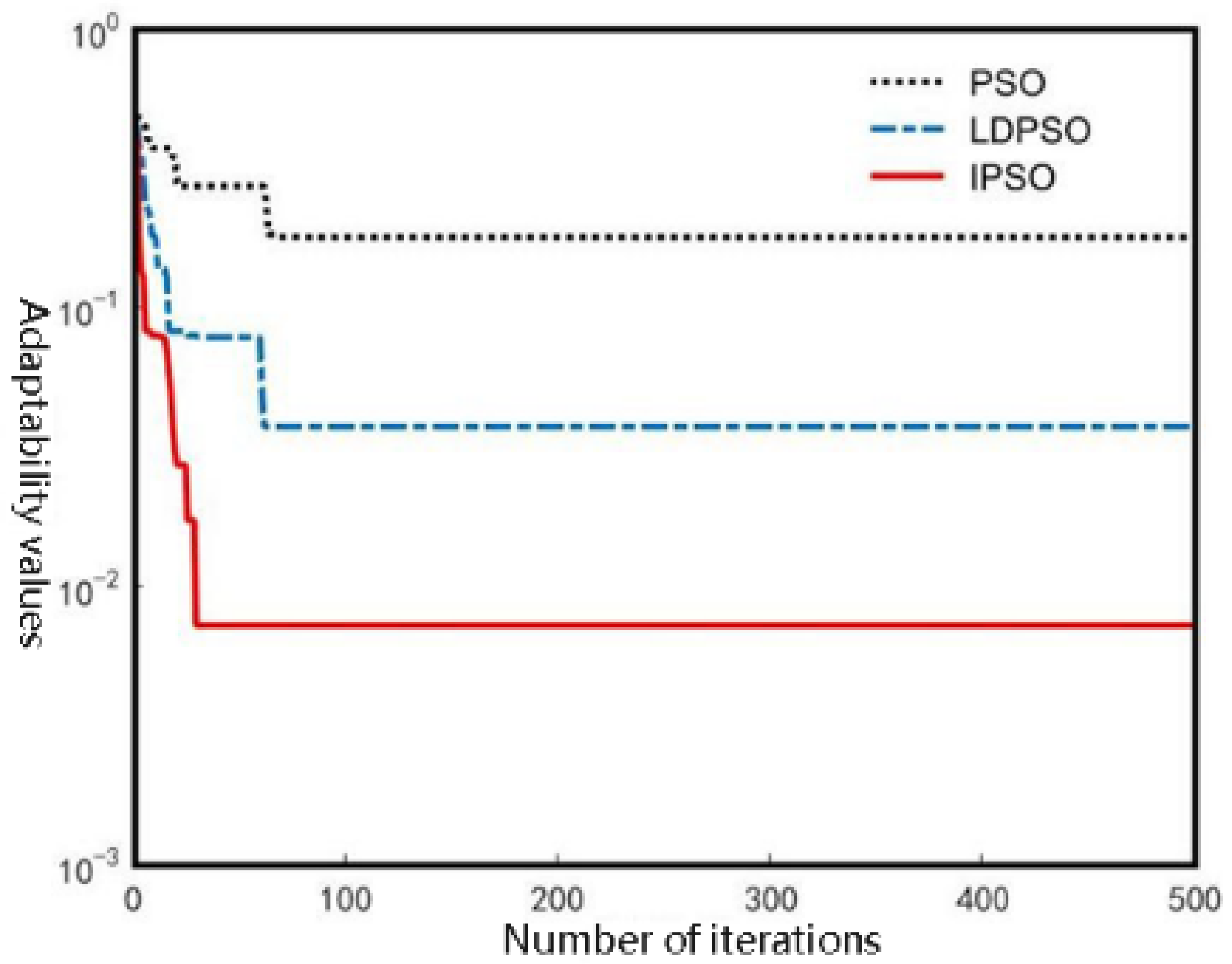
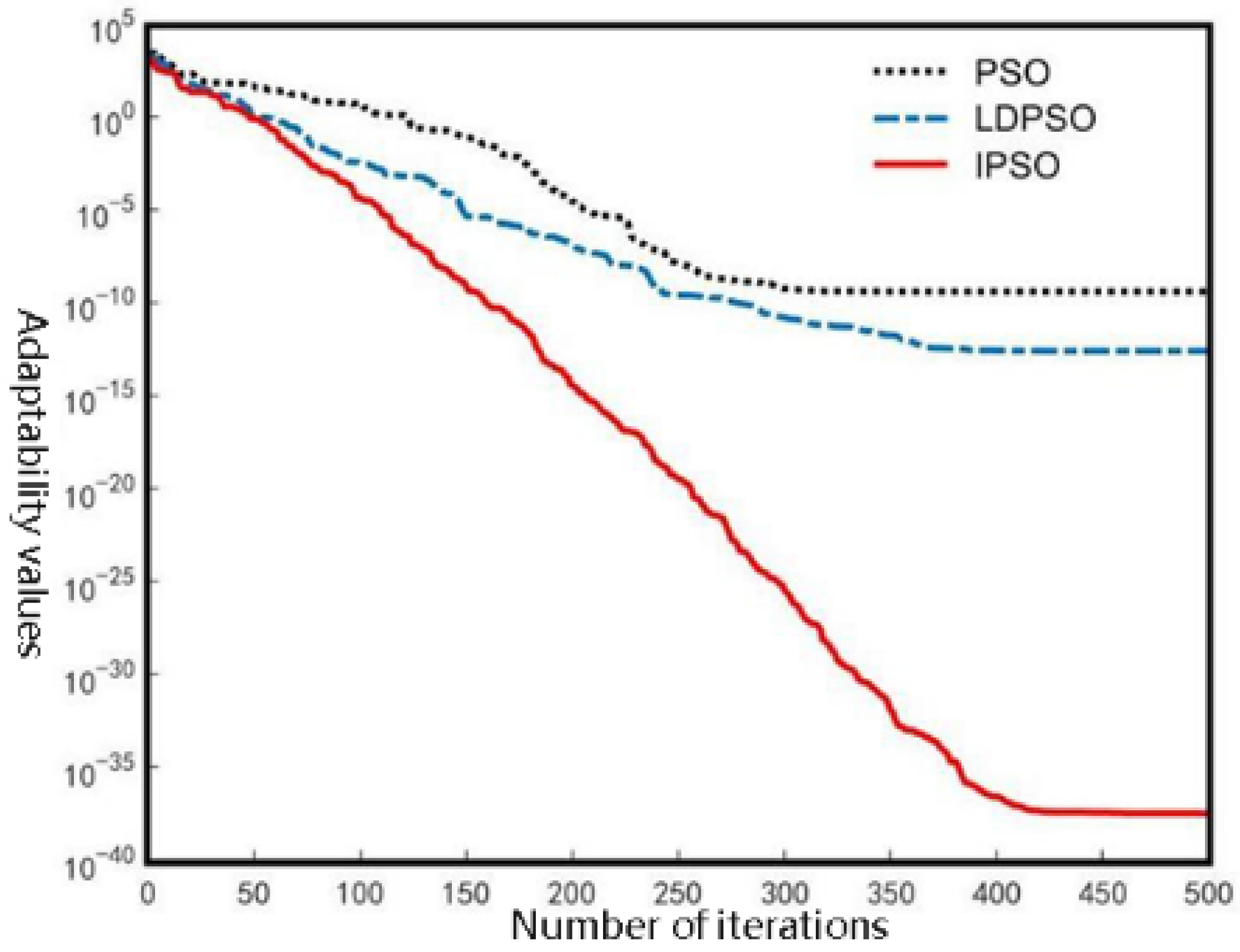
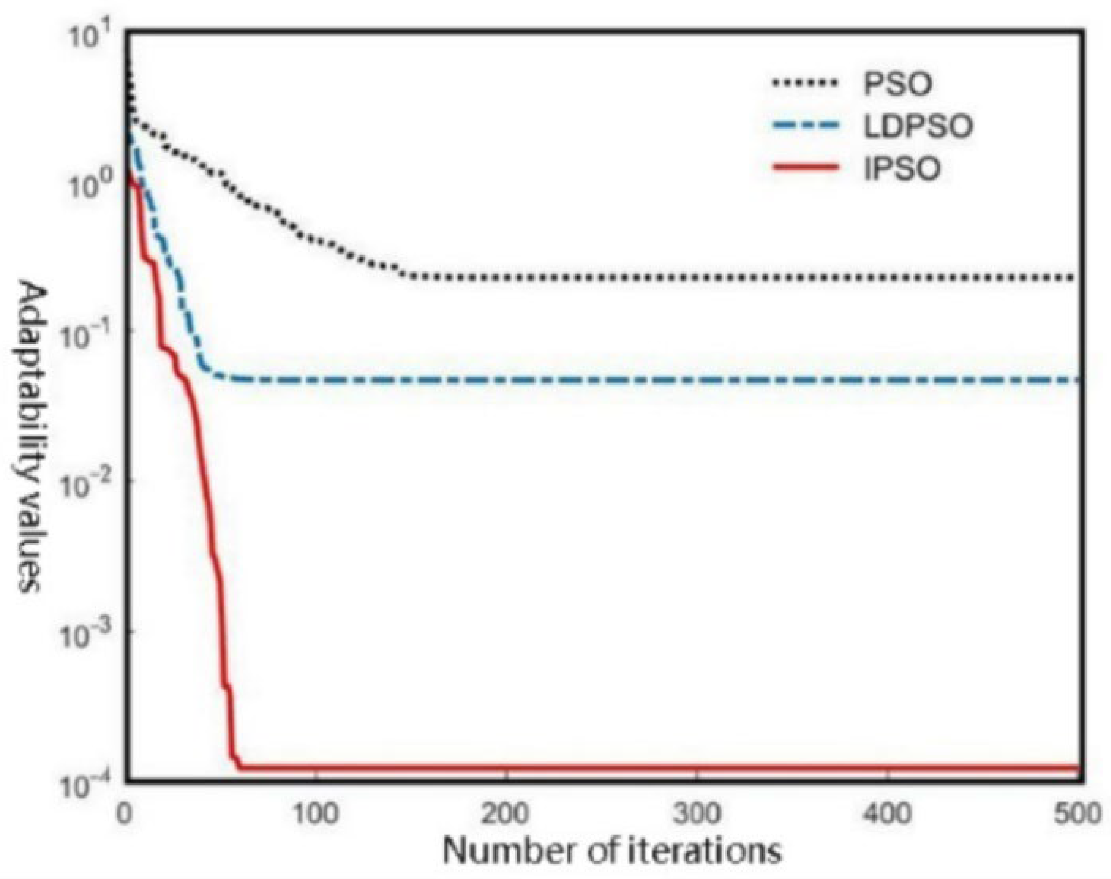
To verify the performance of the improved particle swarm algorithm in dealing with complex problems, the PSO algorithm based on dynamic adjustment of non-linear parameters (IPSO), and the PSO algorithm with linearly decreasing inertia weights (LDPSO), and the standard PSO algorithm was tested using the test functions mentioned above. The convergence curves of the three algorithms for the Sphere function, the Schwefel 1.2 function and the Schaffer function are shown in Figure 1, Figure 2 and Figure 3, respectively.
From the function convergence curves in the above figures, it can be seen that compared with the PSO algorithm and the LDPSO algorithm, the IPSO algorithm has an advantage in convergence accuracy and speed on the Sphere single-peak function and the Schwefel 1.2 single-peak function, and the IPSO algorithm has a more desirable search capability on the Schaffer multi-peak function.
To eliminate the influence of randomness on algorithm performance and quantify algorithm performance reasonably, the three algorithms are independently run 30 times on the MATLAB software. The optimum (Fbest), mean (Mean) and standard deviation (Std) of each algorithm are calculated, and the results are compared and analyzed. Table 2 shows the data obtained.
Combining the optimization results of the standard PSO algorithm, LDPSO algorithm and IPSO algorithm on unimodal and multimodal functions, it can be seen that within the 500 iterations set by the algorithm, the IPSO algorithm performs well on the Sphere function, Schwefel 1.2 function and Schaffer function. The optimal value optimized by the IPSO algorithm is always better than the standard particle swarm optimization algorithm and LDPSO algorithm. At the same time, its optimized mean and variance are also better than standard particle swarm optimization and LDPSO algorithm. This demonstrates that the algorithm’s ideal target value is more likely to be the actual optimal value and its convergence accuracy is more trustworthy.
The above analysis shows that the inclusion of dynamically adjustable inertia weights and learning factors in the IPSO algorithm ensures strong global exploration performance of the particles in the search region in the early stage of particle swarm evolution. At the end of the iteration, the local search ability of the particles is enhanced, thus improving the convergence performance of the algorithm. As a result, the IPSO algorithm’s overall performance is improved. Its search performance and convergence speed are also improved on the single-peak test benchmark function and multi-peak test benchmark function.

3.3. A hybrid Model of PCA-IPSO-ELM

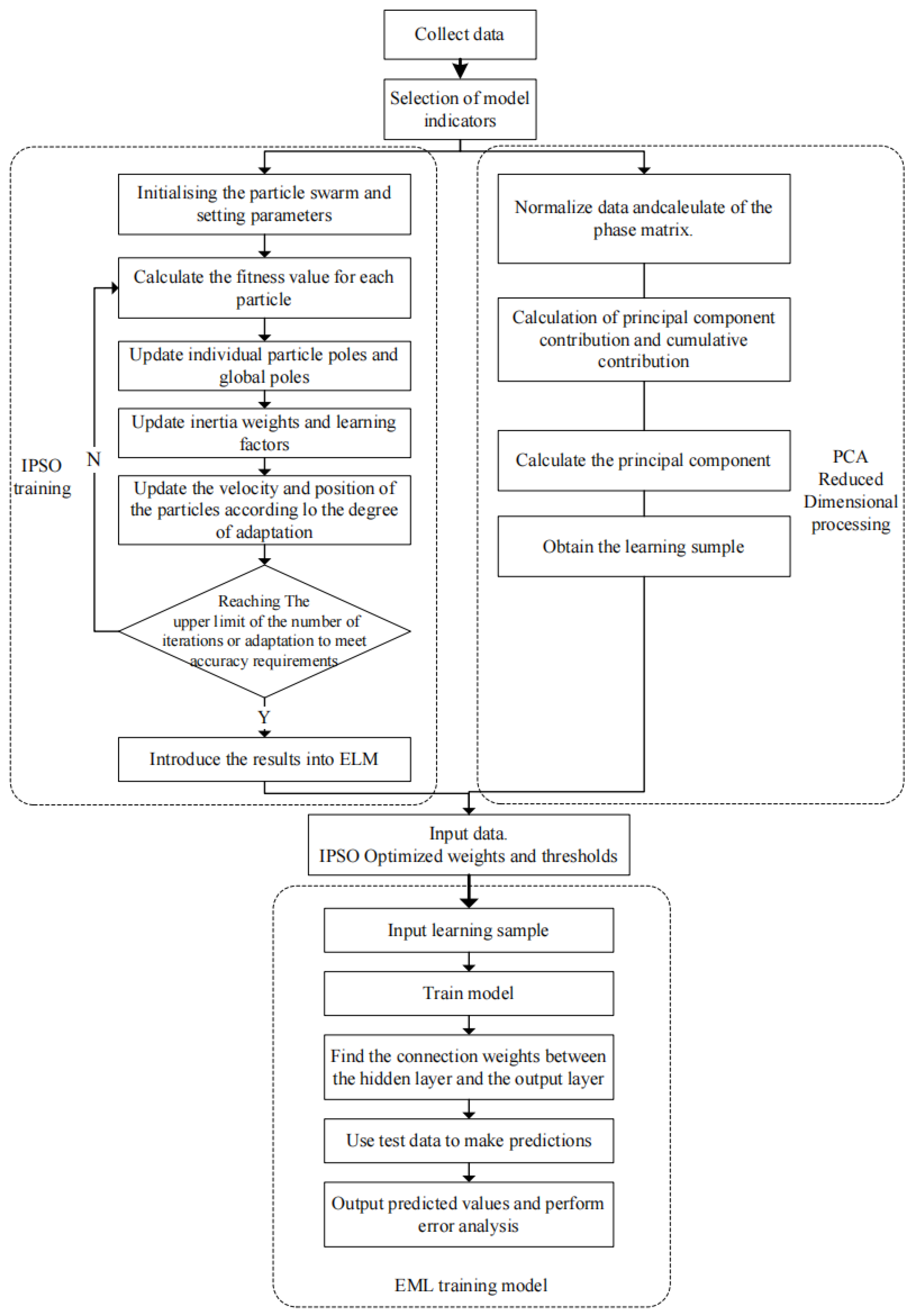
Aiming to solve the problem that the traditional particle swarm algorithm tends to converge prematurely, an improved particle swarm optimization algorithm (IPSO) is introduced, and the extreme learning machine (ELM) is optimized to select the best set of weights and thresholds. At the same time, to eliminate the redundancy of the original data samples due to the multiple factors affecting berthing operation time, which appears to damage the prediction model’s accuracy, the principal component analysis (PCA) is employed to reduce the dimension of the data. Therefore, a hybrid prediction model based on PCA and ELM optimized by IPSO (namely PCA-IPSO-ELM) is proposed to predict the operation time of container ship at berth. The following are the precise steps of the PCA-IPSO-ELM model.
(1) Data preprocessing. New composite indicators are chosen after dimensionality reduction of the multi-factor indicators affecting the operation time of container ships at berth.
(2) The prediction model’s input is derived from the principal component analysis after dimensionality reduction.
(3) The set of parameters to initialize the particle swarm. The specific parameters include particle swarm size, particle velocity and position, set each parameter.
(4) Based on the set objective function, find the fitness value f i of the particle, compare the fitness value f i of the particle with the individual optimal value P b e s t i , if f i > P b e s t i , then P b e s t i = f i ; compare the individual optimal value P b e s t i with G b e s t i , if   P b e s t i > G b e s t i , then G b e s t i = P b e s t i , and find the global optimal value.
(5) Update the individual extremum and global extremum of the particle; update the inertia weight and learning factor; and update the speed and position of the particle according to the fitness value.
(6) Repeat the above steps until the upper limit of the number of iterations is reached or the accuracy requirement is satisfied.
(7) The optimal particle positions derived in the extreme learning machine are the corresponding optimal input weights and hidden layer thresholds, and the output weight matrix is calculated. The obtained optimal results are used for training the ELM model, and evaluating the model. The PCA-IPSO-ELM model of the container ship berthing operation time forecasting process is shown in Figure 4.

4. Experiment and Discussion

4.1. Data Preprocessing

It can be seen from Section 2.1 that there are 11 uncertain factors identified in this paper, including ship types, and so on. The influencing factors identified in the study are the number of shore bridge X 1 , the number of 20-foot containers unloaded X 2 , the number of 20-foot containers loaded X 3 , the number of 40-foot containers unloaded   X 4 , the number of 40-foot containers loaded   X 5 , the number of special containers unloaded X 6 , the number of special containers loaded X 7 , the type of vessel X 8 , the time of vessel berthing   X 9 , the number of collector trucks X 10 , the number of yard bridges   X 11 , and the weather (wind level and rain and snow) X 12 . In this study, it is assumed that each quay bridge, field bridge, and collecting card performs the same amount of work per unit of time. Since some categories in the original data are represented by words, it is necessary to code and process the text records of ship type and weather, while also digitally converting the time series of berthing time.
The data samples obtained by the coding procedure are shown in Table 3, which randomly selects 1000 data from the original data. In order to ensure that the prediction is accurate, 700 samples from the training set and 300 samples from the test set must be randomly generated in the ratio of 7:3. The container ship operation information sheet is shown in Table 4.
Before conducting principal component analysis, the original samples were first analyzed to confirm whether they met the requirements of principal component analysis. In this study, the port ship operation data are analyzed by Pearson correlation analysis using IBM SPSS Statistics.
This study uses KMO and Bartlett’s spherical test. The degree of correlation between variables is assessed according to the judgment and the suitability of the sample data when using principal component analysis method. The results of the test are displayed in Table 5 with a significance level of 0.000 and a KMO measure of 0.717. The resultant value of the method satisfies the KMO measure’s requirements as well as the significance level of Bartlett’s sphericity test below 0.01. The analysis demonstrates that the original data’s parameters show a strong correlation, and the chosen sample data satisfies the necessary conditions for the principal component analysis approach, which may be used to reduce dimensionality.
Using the MATLAB software, principal component analysis is carried out on the container ship’s berth operation time data. Principal component analysis is performed on the original samples using the princomp function after they have been first normalized with the zscore function. A control group is added to the zscore function standardization of the container ship at berth operation data shown in Table 4 to confirm the logic and validity of the zscore standardization process. In the control group, the steps of the zscore standardization process are skipped, but other conditions are keeping constant. This allows us to assess the logic and validity of the zscore standardization process.
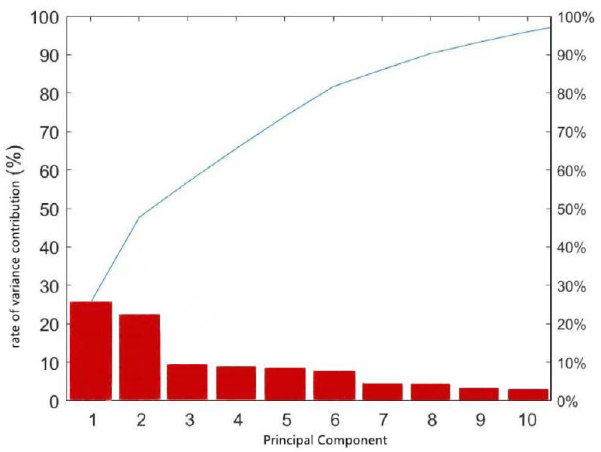
The data information on the number of different types and sizes of containers loaded and uploaded has become the main data of the container ship’s berthing operation data. It is discovered when performing principal component analysis on the data of the control group, it is found that because its values are significantly higher than other data indicators. Because of this, both the size of the coefficient matrix and the size of difference between each primary component’s contribution rate are too large. It is therefore determined that the magnitude difference of the coefficient matrix of principal component analysis will be too big when the original data are not standardized by the zscore function, which will damage the outcome of experimental data analysis. Therefore, using the zscore standardization step can eliminate the negative impact of different index magnitudes in the original data on the model effect, and reduce the impact of high-level numerical indicators on low-level numerical indicators. Additionally, this method can also avoid the impact of some higher value indicators on the main data sample score. Following zscore normalization, Figure 5 displays the principle component variance contribution rate.
Figure 5 illustrates the contributions of each principal component and the variance of each principal component on the horizontal and vertical axes, respectively. A bar graph displays the variance contributions of each principal component. The eigenvalues of each variable in Figure 5 are sorted from largest to smallest, and the cumulative contribution of the first seven principal components, F1, F2, F3, F4, F5, F6, F7, is over 85%, meeting the standard of covering the main information in the original sample. Therefore, the principal component matrix can be obtained from the above seven eigenvalues. The 7-D principal component matrix retains the main information of the original data and eliminates the irrelevant information. Table 6 shows the composition matrix. Seven principal component calculation formulas composed of 12 influencing factors can be obtained from the table. Each column of numbers corresponds to the coefficient of each factor. Thus, principal component analysis reduces the complexity of the data and produces more condensed and informative data samples for the next stage of training the prediction model by replacing the muti-indicators of high-dimensional samples with low-dimensional and comprehensive indicators.

4.2. Parameters Setting of PCA-ELM-IPSO Model

In this section, we use the principal component matrix as the input matrix for the container ship berthing operation prediction model experiments, and use the actual berthing operation time as the output variable. Besides, we also use the MATLAB tool for model training and prediction.
In this paper, the parameters of particle swarm optimization algorithm, extreme learning machine and principal component analysis are shown in Table 7. The number of nodes in the implicit layer in the limit learning machine is determined by the formula l = n + m in Section 4.1 (l, n and m are the number of nodes in the implicit layer, input layer and output layer, respectively, and a is a constant, which is generally taken in the range of [1,10 ] ). To find the optimal number of nodes in the hidden layer, the study is evaluated by the magnitude of the mean square error under the same data samples and experimental conditions. After training, it is found that the model means square error is minimized when the number of nodes in the hidden layer was 11. As a result, the number of nodes in the hidden layer is set to 11, the number of neurons in the output layer is set to 1, the Sigmoid function is chosen as the activation function, and the smoothing factor   k controlling the smoothness of the ω curves is set to 0.7, and the smoothing factor m controlling the smoothness of the c 1 and c 2 curves is set to 2. In addition, to ensure the accuracy of the prediction, Section 4.1 needs to generate 700 training set samples and 300 test set samples at a random ratio of 7:3 when pre-processing the data.

4.3. Analysis of Prediction Results

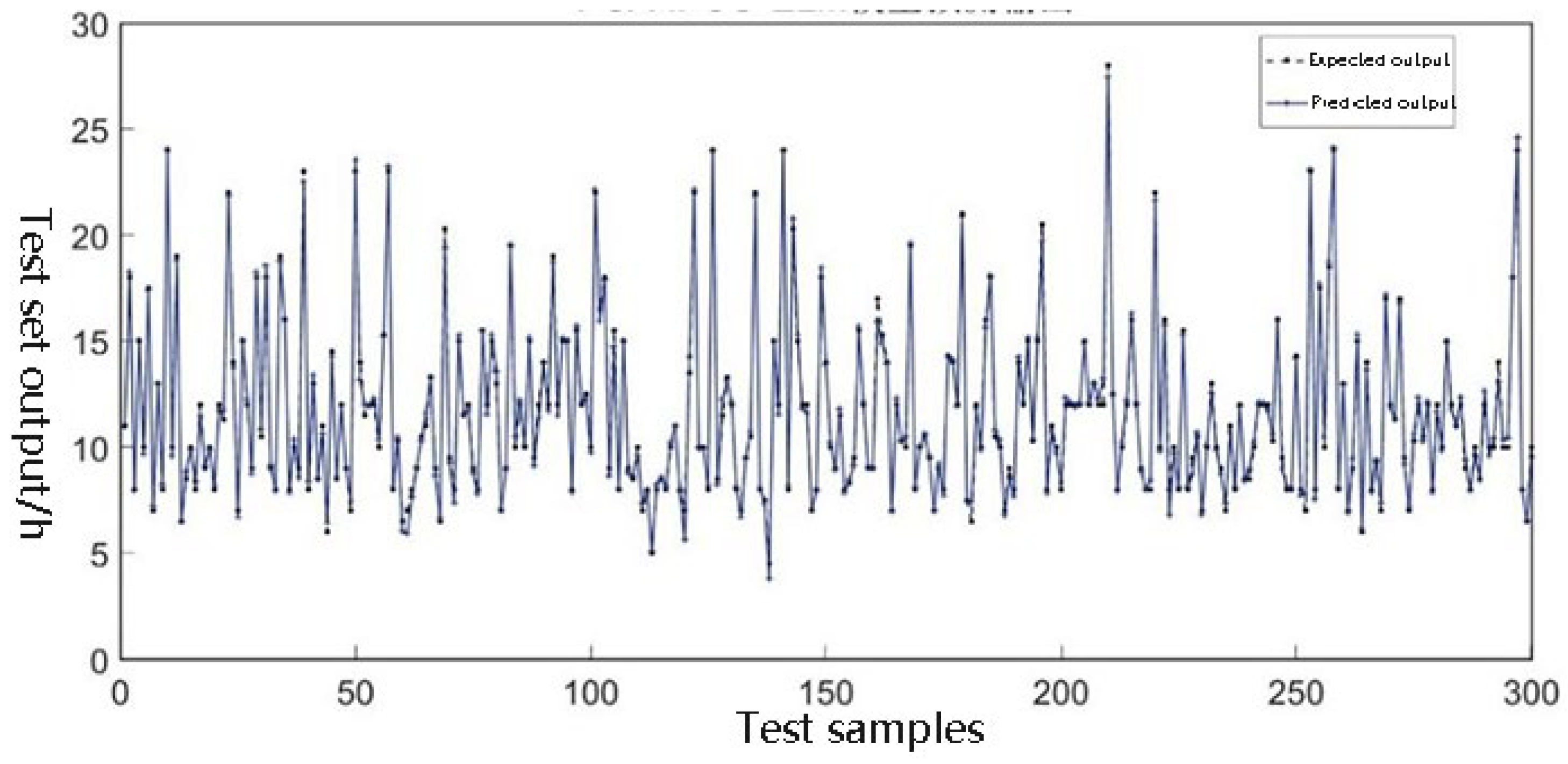
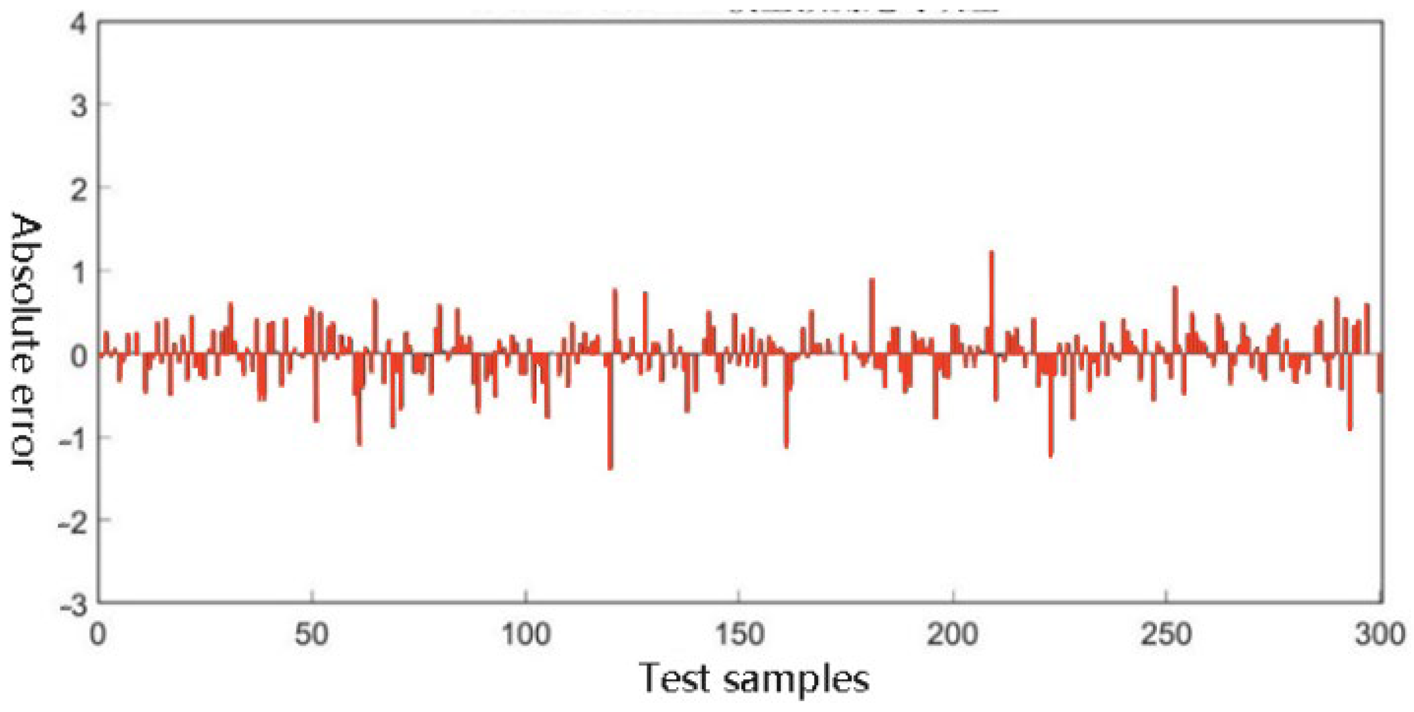
Combining principal component analysis, improved particle swarm optimization, and extreme learning machine algorithm, a prediction model of container ship berth operation time based on PCA-IPSO-ELM is established. The data samples after dimensionality reduction by principal component analysis are selected, and the training and prediction of the PCA-IPSO-ELM model are carried out by the MATLAB software. Figure 6 shows the predicted and true values of the hybrid PCA-IPSO-ELM model, and Figure 7 shows the absolute error of the model prediction.
In Figure 6, the black dotted line indicates the expected output value, and the blue solid line indicates the predicted output of the model. The predicted trend is consistent with the actual container ship’s berth operation, and the fitting degree of the model is good. At the same time, it can be seen from Figure 7 that the absolute prediction error of the PCA-IPSO-ELM model is generally in a low floating range. It can be inferred that this model has good prediction performance in predicting the berth operation time of container ships.
In order to further verify the effectiveness of the PCA-IPSO-ELM prediction model, the standard BP neural network model, ELM model, GA-BP neural network model, and the IPSO-ELM model are selected as comparison experiments. Among them, the excitation function of the hidden layer of the BP neural network is Sigmoid, the excitation function of the output layer is Purelin, the number of neurons in the hidden layer is 10, the maximum number of training is 500, the accuracy requirement is set to 0.0001, the learning rate is 0.01, the weights and thresholds of the network are initialized to a value between them, the chromosome coding length in GA is 168, the population size is set to 60, the evolution algebra is 30, and the crossover probability is 0. The BP, ELM, GA-BP, and IPSO-ELM models are programmed using the MATLAB platform to complete the training process of the models, and the test set is predicted and analyzed.
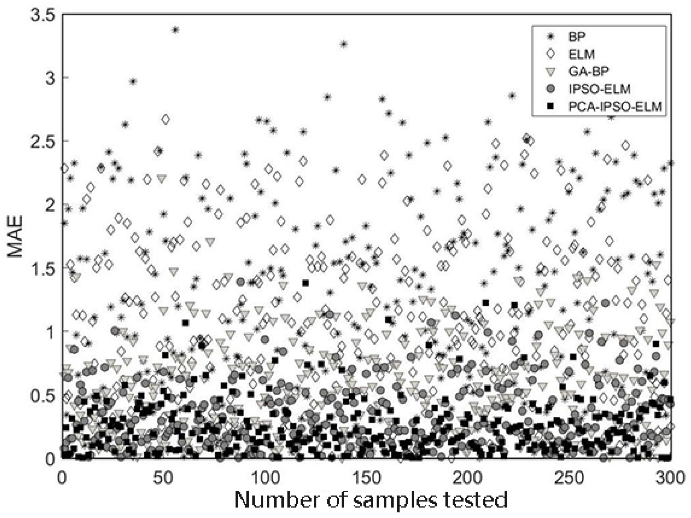
The prediction results of the PCA-IPSO-ELM model proposed in this paper are compared with the other four models, and it is finds that the single BP neural network model has the worst prediction effect and the biggest error. Compared with the standard BP neural network, the GA-BP model improves the prediction accuracy, but the iteration speed is slow and the solution process takes a long time. The PCA-IPSO-ELM model proposed in this paper has the best fitting effect, and the absolute error of prediction is mainly concentrated in the interval, while the IPSO-ELM model is second only to PCA-IPSO-ELMEL model. The prediction results of the above five groups of models are BP < ELM < GA-BP < IPSO-ELM < PCA-IPSO-ELM. To further analyze the comprehensive performance of the prediction models, the training is repeated 30 times, and the average absolute error, root mean square error, determination coefficient and running time are used to predict the BP, ELM, IPSO-ELM, GA-BP and PCA-IPSO-ELM models. The prediction results of the IPSO-ELM model are analyzed, and the results are shown in Table 8. The absolute error comparison of the five models is shown in Figure 8.
From the comparison results of the prediction data of the five models, we can conclude that:
(1) The average absolute error and root mean square error of the PCA-IPSO-ELM model are 0.3196 and 0.4080, respectively, which are lower than 1.3508 and 1.4913 of BP model, 1.0929 and 1.2761 of ELM model, 0.5672 and 0.6884 of GA-BP model, and 0.3581 and 0.4759 of IPSO-ELM model. The coefficient of determination of the PCA-IPSO-ELM model is 98.62%, which is higher than 87.31% for the BP model, 90.55% for the ELM model, 95.06% for the GA-BP model, and 97.79% for the IPSO-ELM model.
(2) According to the analysis of the running time of the different models, the running time of the ELM model is 458.072 s, while that of BP model is 932.697 s, which is about twice that of BP. On this basis, the PCA-IPSO-ELM model has a running time of 201.787 s, which is also faster than the GA-BP model with 615.406 s and the IPSO-ELM model with 228.593 s, requiring the shortest running time.
By analyzing the performance of the five prediction models, the PCA-IPSO-ELM model has the smallest prediction error, the best fitting degree, and the shortest running time. It can be concluded that compared with the single BP neural network model, the performance of ELM model is improved, but the prediction accuracy and fit of the two models are still insufficient. Compared with the GA-BP model and other three models, the PCA-IPSO-ELM model avoids the influence of redundant data, and effectively overcomes the shortcomings of common prediction models, such as slow response, premature convergence to local optimum and excessive memory consumption.
5. Conclusions

The projected berthing time of container ships is an important basis for making berth plans. An accurate prediction can effectively improve the utilization of berthing resources, thus improving the operational efficiency and service level of ports, and achieving a win-win situation for the port, shipping companies and cargo companies. It has important practical significance for the actual production and operation of ports. With the goal of improving the comprehensiveness of the prediction model, a hybrid prediction model based on principal component analysis and improved particle swarm optimization (PCA-IPSO-ELM) is proposed for optimizing extreme learning machines by studying the variables affecting the berthing time of container ships under uncertain conditions. Moreover, the variables affecting the operation time of container ships at berth are analyzed and the port operation data of Tianjin Port Container Ship Company are pre-processed by dimensionality reduction preprocessing. Standard Particle Swarm Optimization (PSO) suffers from the problems of easily falling into local optimum prematurely, relatively unbalanced global and local search capabilities, and slow convergence during the optimization process. Aiming at the above problems, this paper proposes an improved PSO algorithm based on the dynamic adjustment of nonlinear parameters. The verification results show that the improved particle swarm optimization algorithm is superior to the basic particle swarm optimization algorithm and linear decreasing weight particle swarm optimization algorithm in the aspects of optimal value, mean value, and standard deviation. Based on the research of the improved particle swarm optimization algorithm, the extreme learning machine is optimized by using the improved algorithm. Additionally, the best combination of weights and threshold is selected to improve the prediction performance of the model.
Finally, taking Tianjin Port Container Line as an example, we compare the prediction results of the traditional BP, ELM, GA-BP, and IPSO-ELM models. We can know that the average absolute error, root mean square error and running time of the PCA-IPSO-ELM prediction model are 0.3196 h, 0.4080 h and 201.787 s, respectively, all of which are lower than the corresponding indexes of other models; and the coefficient of determination of our model is 98.62%, which is higher than other models. The experiment verifies that the PCA-IPSO-ELM-based container ship at berth operation time prediction model proposed in this study has good prediction performance and can provides a decision basis for optimal allocation of container port resources. There is room for further study and improvement. In this paper, principal component analysis is used to reduce the dimensionality of the original index data, and further research is needed to find a better data processing method than PCA to make full use of data information resources.

Author Contributions

Conceptualization, Z.L.; Methodology, Z.L. and L.W.; Validation, W.P.; Formal analysis, L.W., W.P. and S.D.; Investigation, W.P., S.D. and J.Z.; Resources, S.D.; Data curation, S.D.; Writing—original draft, L.W., W.P. and S.D.; Writing—review & editing, Z.L., H.J. and J.Z.; Visualization, L.W.; Supervision, Z.L.; Project administration, Z.L. and H.J.; Funding acquisition, H.J. All authors have read and agreed to the published version of the manuscript.

Funding

This work was supported by the Science and Technology Foundation of Liaoning Provincial Education Department, China (Grant No. LJKZ1352).

Institutional Review Board Statement

Not applicable.

Informed Consent Statement

Not applicable.

Data Availability Statement

The data presented in this study are available upon request.

Conflicts of Interest

The authors declare no conflict of interest.

References

  1. Dulebenets, M.A. Minimizing the Total Liner Shipping Route Service Costs via Application of an Efficient Collaborative Agreement. IEEE Trans. Intell. Transp. Syst. 2018, 20, 123–136. [Google Scholar] [CrossRef]
  2. Lin, H.; Yang, L.; Luan, H.; Han, C.; Han, P.; Xu, H.; Chen, G. A data-driven assessment model for collision responses of offshore platform structure with ship using hybrid intelligent approaches. Process Saf. Environ. Prot. 2022, 167, 225–246. [Google Scholar] [CrossRef]
  3. Dulebenets, M.A. A comprehensive multi-objective optimization model for the vessel scheduling problem in liner shipping. Int. J. Prod. Econ. 2018, 196, 293–318. [Google Scholar] [CrossRef]
  4. Gollas, M.M. A bi-objective berth allocation formulation to account for vessel handling time uncertainty. Marit. Econ. Logist. 2011, 13, 419–441. [Google Scholar] [CrossRef]
  5. Chen, J.; Wang, Y.; Yu, X.; Liu, Z. Integrated Optimization of Port Rotation Direction and Fleet Deployment for Container Liner Shipping Route. Hindawi Discret. Dyn. Nat. Soc. 2021, 2021, 3592460. [Google Scholar] [CrossRef]
  6. Mohammadi, M.; Forghani, K. Solving a stochastic berth allocation problem using a hybrid sequence pair-based simulated annealing algorithm. Eng. Optim. 2019, 51, 1810–1828. [Google Scholar] [CrossRef]
  7. Rodriguez-Molins, M.; Salido, M.A.; Barber, F. Robust Scheduling for Berth Allocation and Quay Crane Assignment Problem. Hindawi Math. Probl. Eng. 2014, 2014, 834927. [Google Scholar] [CrossRef]
  8. Yu, F.F.; Shan, Q.H.; Xiao, Y.; Teng, F. Robust Low-Carbon Discrete Berth Allocation under Uncertainty. Hindawi Int. Trans. Electr. Energy Syst. 2022, 2022, 5310004. [Google Scholar] [CrossRef]
  9. Liu, W.; Zhu, X.; Wang, L.; Li, S. Rolling horizon based robust optimization method of quayside operations in maritime container ports. Ocean. Eng. 2022, 256, 111505. [Google Scholar] [CrossRef]
  10. Zhao, H.W.; Liu, Y.Q.; Huang, Y.P.; Xuwang, L.; Xiaohang, T. Short-term free parking berths prediction based on multitask—DBN neural network. J. Intell. Fuzzy Syst. 2019, 37, 4493–4498. [Google Scholar] [CrossRef]
  11. Li, B.; He, Y.Q. Container Terminal Liner Berthing Time Prediction with Computational Logistics and Deep Learning. In Proceedings of the 2020 IEEE International Conference on Systems, Man, and Cybernetics (SMC), Toronto, ON, Canada, 11–14 October 2020; pp. 2417–2424. [Google Scholar]
  12. Bakar, N.N.A.; Bazmohammadi, N.; Çimen, H.; Uyanik, T.; Vasquez, J.C.; Guerrero, J.M. Data-driven ship berthing forecasting for cold ironing in maritime transportation. Appl. Energy 2022, 326, 119947. [Google Scholar] [CrossRef]
  13. Farag, Y.B.A.; Ölçer, A.I. The development of a ship performance model in varying operating conditions based on ANN and regression techniques. Ocean. Eng. 2020, 198, 106972. [Google Scholar] [CrossRef]
  14. Chen, Y.R.; Dong, Z.K.; Wang, Y.; Su, J.; Han, Z.L.; Zhou, D.; Zhang, K.; Zhao, Y.S.; Bao, Y. Short-term wind speed predicting framework based on EEMD-GA-LSTM method under large scaled wind history. Energy Convers. Manag. 2021, 227, 113559. [Google Scholar] [CrossRef]
  15. Ma, M.; Yao, H.; Liu, H.C.; Tang, Z. State of Health estimation and Remaining Useful Life prediction for lithium-ion batteries by Improved Particle Swarm Optimization-Back Propagation Neural Network. J. Energy Storage 2022, 52, 104750. [Google Scholar] [CrossRef]
  16. Park, Y.M.; Kim, K.H. A scheduling method for berth and quay cranes. In Container Terminals and Automated Transport Systems; Springer: Berlin/Heidelberg, Germany, 2005; pp. 159–181. [Google Scholar]
  17. Gui, X.Y. Integrated optimization for berth and quay crane scheduling in container terminals under uncertainty. Master’s Thesis, Shanghai Jiaotong University, Shanghai, China, 2013. (In Chinese). [Google Scholar]
  18. Peng, Y.; Liu, H.K. Chapter 2—Simulation application in port. In Port Planning and Management Simulation; Elsevier: Amsterdam, The Netherlands, 2022; pp. 23–46. [Google Scholar]
  19. Zhen, L.; Zhuge, D.; Wang, S.A.; Wang, K. Integrated berth and yard space allocation under uncertainty. Transp. Res. Part B Methodol. 2022, 162, 1–27. [Google Scholar] [CrossRef]
  20. Wang, J.; Guo, L.M.; Du, J. Wang, M. Dynamic learning based berth scheduling scheme optimization. Transp. Syst. Eng. Inf. 2018, 18, 197–203. [Google Scholar]
  21. Han, Z.B.; Xu, B.; Chen, J. Neural network-based port operation time prediction model for container ships. Comput. Appl. Softw. 2021, 38, 78–84. [Google Scholar]
  22. Rumelhart, D.E.; Hinton, G.E.; Williams, R.J. Learning Representations by Back Propagating Errors. Nature 1986, 323, 533–536. [Google Scholar] [CrossRef]
  23. Huang, G.-B.; Zhou, H.; Ding, X.; Zhang, R. Extreme Learning Machine for Regression and Multiclass Classification. IEEE Trans. Syst. Man Cybern. Part B 2012, 42, 513–529. [Google Scholar] [CrossRef] [Green Version]
  24. Parida, M.; Behera, M.K.; Nayak, N. Combined EMD-ELM and OS-ELM techniques based on feed-forward networks for PV power forecasting. In Proceedings of the 2018 Technologies for Smart-City Energy Security and Power (ICSESP), Bhubaneswar, India, 28–30 March 2018; pp. 1–6. [Google Scholar]
  25. Jia, Z.; Song, Z.; Fan, J.; Jiang, J. Prediction of Blasting Fragmentation Based on GWO-ELM. Shock. Vib. 2022, 2022, 85456. [Google Scholar] [CrossRef]
  26. Wei, X.; Liu, H.; She, X.; Lu, Y.; Liu, X.; Mo, S. Stability Assessment of Rubble Mound Breakwaters Using Extreme Learning Machine Models. J. Mar. Sci. Eng. 2019, 7, 312. [Google Scholar] [CrossRef] [Green Version]
  27. Chai, G.A.; Wu, J.H.; Yao, L.; Zang, Q. Optimization of combined cooling, heating and power type microgrid operation based on improved dynamic inertia weighted particle swarm algorithm. Sci. Technol. Eng. 2022, 22, 1472–1479. [Google Scholar]
  28. Gao, D.; Zhou, P.; Shi, W.F.; Wang, T.; Wang, Y. A Dynamic Obstacle Avoidance Method for Unmanned Surface Vehicle under the International Regulations for Preventing Collisions at Sea. J. Mar. Sci. Eng. 2022, 10, 901. [Google Scholar] [CrossRef]
  29. Bian, Y.; Yan, W.; Hu, H.; Li, Z. Feeder Scheduling and Container Transportation with the Factors of Draught and Bridge in the Yangtze River, China. J. Mar. Sci. Eng. 2021, 9, 964. [Google Scholar] [CrossRef]
  30. Zheng, Q.; Feng, B.W.; Liu, Z.Y.; Chang, H.C. Application of Improved Particle Swarm Optimisation Algorithm in Hull form Optimisation. J. Mar. Sci. Eng. 2021, 9, 955. [Google Scholar] [CrossRef]
  31. Mosa, M.A.; Anwar, A.S.; Hamouda, A. A survey of multiple types of text summarization with their satellite contents based on swarm intelligence optimization algorithms. Knowl. Based Syst. 2019, 163, 518–532. [Google Scholar] [CrossRef]
Figure 1. Convergence of Sphere function.
Jmse 10 01919 g001
Figure 2. Convergence of Schwefel 1.2 function.
Jmse 10 01919 g002
Figure 3. Convergence of Schaffer function.
Jmse 10 01919 g003
Figure 4. Flow chart of PCA-IPSO-ELM model.
Jmse 10 01919 g004
Figure 5. Principal component variance contribution rate.
Jmse 10 01919 g005
Figure 6. Comparison of predicted value and expected value of PCA-IPSO-ELM model.
Jmse 10 01919 g006
Figure 7. PCA-IPSO-ELM model prediction absolute error diagram.
Jmse 10 01919 g007
Figure 8. Comparison chart of absolute error of algorithm prediction.
Jmse 10 01919 g008
Table 1. Algorithm parameters.
AlgorithmsParameter Settings
Standard Particle Swarm
Algorithm (PSO)
ω = 0.7298 , c 1 = c 2 = 1.496
ω Linearly decreasing particle swarm algorithms (LDPSO) ω m a x = 0.9 , ω m i n = 0.4 , c 1 = c 2 = 1.496
Improved particle swarm algorithm (IPSO) ω m a x = 0.9 , ω m i n = 0.4 ,  k = 0.7, m = 2
Table 2. Results of the test function.
FunctionsAlgorithmsFbestMeanStd
Sphere functionPSO3.730 × 10−104.280 × 101250.016
LDPSO2.394 × 10−132.450 × 101162.180
IPSO3.407 × 10−381.184 × 10183.9579
Schwefel functionPSO2.262 × 10−14.487 × 10−10.630
LDPSO4.674 × 10−29.570 × 10−20.260
IPSO1.212 × 10−42.365 × 10−20.130
Schaffer functionPSO1.782 × 10−11.972 × 10−10.0539
LDPSO3.722 × 10−24.915 × 10−20.0422
IPSO7.226 × 10−31.192 × 10−20.0379
Table 3. Weather types after coding.
WeatherAir VelocityEncoding
Sunny, cloudy, overcastLevel 1–61
Level 6–82
Beijing-Tianjin-Hebei provinceLevel 1–63
Level 6–84
Light rainLevel 1–65
Level 6–86
Yangtze River DeltaLevel 1–67
Level 6–88
Moderate rain, heavy rainLevel 1–69
Level 6–810
Table 4. Container ship operation information sheet.
Serial NumberX1X2X3X4X5X6X7X8X9X10X11X12
111781844045302942.6531
22120921967162129317.5744
316211458594378318423
41411331091336339420.2422
51679540226160222.5325
641704703792901186035.420113
721901949410079445231161
831252071271152833212.51377
10001626032302147510.6321
Table 5. KMO measurement and Bartlett test.
Statistical QuantityNumerical Value
KMO0.717
Bartlett’s spherical test chi-square statistic3944.940
(number of) Degrees of freedom (physics and statistics)66
Saliency0.000
Table 6. Composition matrix.
Variable1234567
X1−0.0170.454−0.0130.1440.240−0.010−0.835
X2−0.0170.420−0.556−0.056−0.0470.0050.107
X30.0190.450−0.452−0.049−0.1090.0010.313
X40.0040.4540.483−0.037−0.108−0.0440.198
X5−0.0150.4490.489−0.051−0.126−0.0530.173
X60.0180.0580.053−0.4890.8310.1680.182
X70.4660.0070.0810.013−0.1120.356−0.067
X80.4200.020−0.053−0.060−0.0650.316−0.047
X90.4490.0180.0140.009−0.0660.3900.016
X10−0.0330.0590.0180.8480.3960.1820.283
X110.460−0.005−0.0330.0530.094−0.4940.033
X120.437−0.012−0.0070.0670.157−0.5580.044
Table 7. Model parameter setting.
ModelParameter Setting
PSOpopulation size100
Maximum number of iterations500
Dimension10
Maximum inertia weight0.9
Minimum inertia weight0.4
Particle velocity interval [ 1 , 1 ]
ELMNodes in the implicit layerdetermined by the formula l = n + m in Section 4.1
PCAinput node7
Output node1
Nodes in the implicit layer [ 4 , 13 ]
Table 8. Prediction model performance analysis.
ModelsMAERMSER2Running Time (s)
BP1.35081.491387.31%932.697
ELM1.09291.276190.55%458.072
GA-BP0.56720.688495.06%615.406
IPSO-ELM0.35810.475997.79%228.593
PCA-IPSO-ELM0.31960.408098.62%201.787
Publisher’s Note: MDPI stays neutral with regard to jurisdictional claims in published maps and institutional affiliations.