The Impact of the Crude Oil Price on Tankers’ Port-Call Features: Mining the Information in Automatic Identification System

Abstract

Ship navigation technical data contains a lot of information. In this paper, we explore a relationship between the crude oil price and tankers’ port-call features by mining the information recorded in Automatic Identification System (AIS), which extends the application field of ship navigation technical data and aims to help oil shipping enterprises and port enterprises to arrange operation plans in advance. We generate a monthly panel data over the period from 2010 to 2020 of major global ports located in main crude oil exporting countries from AIS data. By using the panel fixed-effect model and binary logit model, our empirical results innovatively present the tanker’s monthly port-call features are influenced by crude oil price fluctuation through four dimensions, that is the tankers’ port-call numbers, the average docking time, total gross tonnage of the docking tankers and the number of different docking tankers. With these variables, we attempt to analyze the relationship between crude oil price fluctuation on tankers’ port-call features. The results of the study are helpful to comprehensively understand the impact mechanism of the crude oil price on the tankers’ port-call features.

1. Introduction

Ship navigation data, which includes the location of the vessel, the docking time, vessel types, etc. provides huge information to researchers. The wide application of Automatic Identification System (AIS) makes the research on the ship navigation information come true. AIS is an international maritime security communication system that uses ship tracking equipment to monitor the activities of cargo ships worldwide. The information recorded by AIS includes ship position, speed, course, type and name, etc. Although the original intention of using AIS is to strengthen the personal safety at sea, improve the safety and efficiency of navigation, and protect the marine environment, the valuable information provided by AIS is now successfully used in various fields. For example, Moore, et al. [1] explored ship traffic variability of California; Arslanalp, et al. [2] used this raw data information to predict trade flows; Cerdeiro and Komaromi [3] applied this new big data source to obtain the top 50 routes in terms of non-commodity import forecasts for port performance analysis; and Verschuur, et al. [4] used it as an open-source tool to assess the disruption time and resilience of the ports and to derive vulnerability curves for US ports. In addition, it has also been applied to the areas of fisheries and marine CO₂ emission monitoring. Therefore, mining AIS data is a promising research direction.

With the rapid process of globalization, maritime transportation is continuously the main mode of international trade transportation. According to the latest review of maritime transport [5], international seaborne trade is expected to grow by 4.3% in 2021 as commodity trade and global output continue to recover. Furthermore, the average ratio of international seaborne trade to the global gross domestic product (GDP) has remained in the range of 1% to 2% over the past 20 years, with a compound annual growth rate of 2.9% for seaborne trade, which indicates that maritime trade has undergone a period of prosperity.

As an important component of international trade, crude oil trade has always accounted for a significant share in global energy trade market. According to BP Statistical Review of World Energy [6], the crude oil trade volume around the world in 2021 is 65,061 kb/d and the total consumption reaches 91,078 kb/d, which means the crude oil international trade accounts for about 71.43% of the total oil consumption. Among them, the Middle East as well as Russia and the CIS countries are the main crude oil exporters. As crude oil is still one of the most essential energy sources in the world so far, international crude oil seaborne transportation is always accepted to ensure a sufficient supply of basic industrial production materials for countries throughout the world, with the characteristics of large capacity and long transportation. Therefore, a market of specialized vessels designed for specific routes has been formed, which greatly enriches the international economic cooperation in crude oil resources.

The measurement of the factors influencing the crude oil market and the seaborne transportation market has been a hot topic in global maritime research. In the existing literature, Poulakidas and Joutz [7] suggested that the demand for tanker transportation is a derivative of the demand for crude oil, and thus there is a close economic relationship between the crude oil prices and the freight rates in the tanker shipping market. In the background of globalization, crude oil is one of the most widely traded bulk energy commodities worldwide and its price is often used as a leading indicator to predict price movements in other commodity markets (e.g., metals, ores, and agriculture) and maritime transportation markets [8]. Mou, et al. [9] empirically found that the export cargo flows are stronger than that of the import cargo flows. Hence, with cyclicality, volatility and fluctuations in crude oil prices, crude oil trade can affect tanker freight rates and transportation costs of crude oil and refined products where they are produced or consumed [10]. Thus, it may directly affect the revenue and cash flow of tanker owners and is significant for further estimating the profitability of the tanker industry and future investment decisions.

The rapid development of global crude oil trade impacts lots of aspects in the tanker transportation industry. Moreover, since the volatility of crude oil prices is more closely related to global economic activities, which makes the level of freight rates no longer the only measurement of the tanker transportation market. Hence, in recent years, researches on the relationship between supply and demand for tanker shipping services by analyzing port operations have also intensified. This paper focuses on the characteristics of crude oil seaborne transportation market, with the help of AIS data. We construct a monthly panel data set to study the influence of crude oil price fluctuation on tankers’ port-calls, the docking time, the operating capacity and whether there is a new tanker beginning to transport the oil. The change of those indicators under the influence of oil price is important for port managers to make operating plans which may improve the economic efficiency of the ports.

We attempt to explore the impact of crude oil market price fluctuations on the tankers’ port-call features and clarify the transmission mechanism and the relationship between them. By conducting this empirical study with panel data, we also hope to provide ideas and directions for shipping companies and governmental authorities on the current situation and future expectations of the market and the tanker shipping industry, formulating strategies and energy policies in depth. The contributions of this research are three folds. Firstly, by mining the information in AIS data, this paper obtains the panel data of monthly tankers’ port-call data from January 2010 to December 2020, and creatively uses panel data to analyze the influence of crude oil price on tankers’ port-call features. Panel data can control the heterogeneity of research variables in time and space, and can avoid the problem of multicollinearity. Secondly, with the help of AIS data, this paper obtains many variables that reflect the tankers’ port-call features, such as port-call frequency, average docking time, etc. Combined with the analysis based on panel data, this paper provides an empirical basis for the role of crude oil price fluctuations on tankers’ shipping activities, specifically reflecting the direction and degree of the crude oil prices’ influences on the features of tankers’ port-call. This paper supplements the existing literature from multiple perspectives. Finally, the research conclusion can help oil shipping enterprises to make transportation capacity plans in advance, and can also help port enterprises to arrange operators in advance.

The remaining sections are organized as follows: Section 2 reviews previous studies on the tanker transportation market and the fluctuation of future oil price; Section 3 mainly introduces the data and the methods; Section 4 introduces the empirical results; Section 5 presents the robust test; and finally, Section 6 summarizes this paper.

2. Literature Review

2.1. Influencing Factors of the Tanker Transportation Market

The seaborne transportation of crude oil has begun from the late 19th century, which made it possible to transport crude oil by tankers from producing countries to consumer markets worldwide [7]. As an important form of global energy trade, quantitative research on tanker transportation behavior and maritime crude oil trade should be of great significance [11]. Despite the limited type of commodity transported in this way, it still formed an oligopoly market structure by virtue of its low transportation cost, high concentration of tanker owners and guaranteed transportation safety.

2.1.1. The Research on the Relation between Oil Price and Tanker Transportation

Alizadeh and Nomikos [12] pointed out shipping market is closely related to oil prices. In recent years, there have been many studies focusing on tankers’ shipping activities in response to international oil price changes by selecting loading and discharging ports in different countries and regions. For example, Hänninen and Rytkönen [13] gave us a bird’s eye view of oil transportation and terminal development in the Gulf of Finland. Wilmsmeier and Sanchez [14] analyzed the evolution of port development and governance in Chile since the 1990s. Duru, et al. [15] investigated structural changes and the potential economic impact on tanker shipping with data from tanker traffic in the major U.S. liquid bulk ports. Mou, Xie, et al. [9] analyzed the impact of oil price declines on shipping decisions.

2.1.2. The Research on the Vessels’ Docking Behavior

Today, some characteristics of vessels’ docking behavior are also researched, such as Meng, et al. [16] carried out an in-depth analysis on the problem of port congestion and the cost of port docking; Wu, et al. [17] used AIS data to study the sailing time of ships in narrow channel; Wang and Vogt [18] studied chemical tankers’ call in the port of Houston; Wang, et al. [19] focused on the port calls’ time of liner ship in the navigation route. Moreover, inspired by Ding [20] who proposed a way to minimize transportation costs while studying vessel’s transportation routes, Duru, Clott and Mileski [15] investigated the potential impact of long- and short-term structural changes in the market on tanker transportation based on important ports. Other representative literatures include Sánchez, et al. [21], Ducruet [22], Ganapati, et al. [23] and Notteboom, et al. [24].

The supply and demand of crude oil decide its price, but high prices will frustrate the demand. Hence, we can infer that when international oil prices fluctuate, the tankers’ shipping activities change accordingly. However, the aforementioned studies only focus on single port and lack general significance. Thus, taking the advantages of AIS data and in view of the special characteristics of tanker transportation, this paper takes worldwide major oil-loading ports as the research object and try to explore the mechanism of price fluctuations in crude oil as an indicator of the tankers’ transportation market. Related existing studies concentrating on oil price fluctuations mainly focus on the shock effects on crude oil seaborne trade in the macro-view, but there are still relatively few contents linking crude oil trading market with transportation market from the perspective of tankers’ port-calls, the docking time and the number of operating tankers. Therefore, combined with the current situation of marine transportation in crude oil trading market, this paper tries to conduct an analysis on how the ups and downs of oil price impact the tanker transportation market.

2.2. Relevant Research on Crude Oil Futures Price

As mentioned above, fluctuations in crude oil prices directly spur the changes in market demand, acting on economic activities in countries around the world. However, crude oil spot prices are vulnerable to both demand-side and supply-side shocks [25]. Thus, futures contracts are commonly taken to hedge the trading risk of market uncertainty [26,27] with its better liquidity compared with spot trading. It is also proven that international crude oil futures prices have a one-way guide to spot prices [28], indicating that future contracts can contribute to price discovery by gathering information about the specified commodity [29]. Therefore, crude oil futures price has been widely applied to recent studies on commodity price fluctuation in various fields [8,30,31,32].

Referring to the tanker shipping market, ship owners may have a higher anticipation of oil prices and are more likely to increase their investments and purchase crude oil for inventory [33] so as to capture higher future returns. Moreover, high oil prices may respond to factors such as global demand and supply, and oil suppliers, fearing offsetting gains from their futures positions, will hedge their risk by going short in oil futures to prevent any decline in oil prices from being offset by gains in futures [29]. The world’s major producers use benchmark oil prices from around the world as a reference for pricing their own products.

In summary, since no research has been conducted so far on the mechanism and extent of the tanker transportation market affected by future crude oil price changes, we attempt to explore the general rules of crude oil seaborne transportation by researching on the features of tanker’s port-calls from the supply side of the crude oil market. In order to further investigate a more general micro mechanism of oil price fluctuations on the tankers’ activities, we use the AIS data to sort out a panel data model for empirical analysis.

3. Data and Methods

3.1. Data Source

Based on the latest available OPEC [34] statistical annual reports, this study selected 26 countries and regions, 13 of which are from OPEC (Organization of the Petroleum Exporting Countries) member countries, including Algeria, Angola, Congo, Equatorial Guinea, Gabon, Iran, Iraq, Kuwait, Libya, Nigeria, Saudi Arabia, United Arab Emirates and Venezuela. Then the remaining 13 countries are major crude oil exporting non-OPEC member countries, which involves Brazil, Canada, Colombia, Ecuador, Indonesia, Malaysia, Mexico, Norway, Oman, Qatar, Russia, Sudan and Vietnam.

In this paper, we select the monthly data from January 2010 to December 2020 for the oil loading ports located in the aforementioned countries which involve a total sample of 545 ports. The total gross tonnage of the tankers entering and exiting the first 20 largest oil exporting countries in 2020 are shown in Figure 1. According to recent oil export data, oil exporters are mainly distributed in six regions, that is the Middle East, Russia and CIS countries, West Africa, North America, South America and a small number of Asian and Oceanian countries. In those regions, oil tanker’ loading operations are relatively frequent.

International oil prices experienced ups and downs shocks between 2010 and 2020. In order to explore the changes in crude oil transportation trade before and after the rise and fall of oil prices, we collect monthly tanker AIS data from January 2010 to December 2020, including the IMO number (IMO number refers to a unique identification number that is assigned to the marine vessel in accordance with the requirements of the International Maritime Organization (International Maritime Organization, IMO)). of the tanker, the tanker’s gross tonnage, arrival and departure time, the port the tanker calls, the latitude and longitude time zone of the port, etc. After filtering and identifying the required data, we retrieve the ship’s entry and exit port records.

The data applied in this study is downloaded from Lloyd’s Register. It focuses on ship’s activity near targeted ports, especially ships entering and leaving from port vantage points [2]. Based on the aforementioned information recorded by AIS, we acquire how many times the tankers stop at one port per month (monthly frequency of tankers’ port-calls at one port), the average docking time of the tankers, how many different tankers stop at one port (the number of operating tankers), and the total gross tonnage of the tankers (This paper counts different tankers calling at one port repeatedly. To be specific, if a tanker calls at one port twice in one month, its gross tonnage will be added into the total gross tonnage twice in this month.) calling at the port. From AIS data, we obtain 60,540 different tanker observations, which means there are 60,540 different tankers shipping oil in these ten years totally. The numbers vividly present the distribution of crude oil trade among both OPEC and Non-OPEC member countries. We also acquire crude oil futures prices and other macro data from Clarkson, OPEC and EIA (The U.S. Energy Information Administration).

3.2. Descriptive Analysis

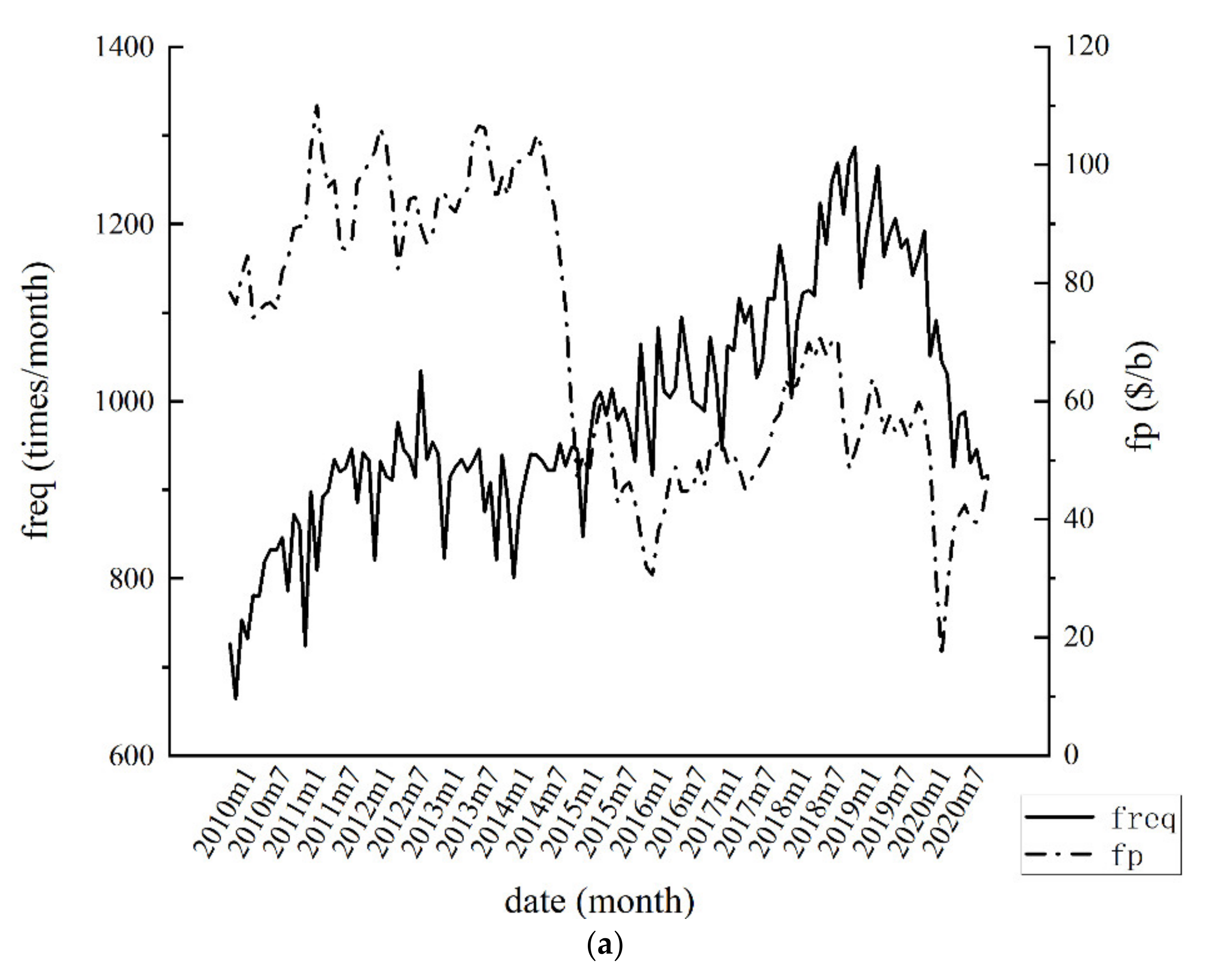
In this paper, we obtain 390,628 real-time records of tankers’ movements based on the major crude oil trade ports around the world with the help of AIS.

Figure 2 illustrates the number of port-calls (indicated by the horizontal axis), the tanker’s average docking time (indicated by the vertical axis) and the monthly average total gross tonnage of the tankers stopping at the 545 ports. The total gross tonnage is shown by circle. It can be found that generally speaking if the total tonnage of all tankers stopped at a port is larger, the number of tankers stopped at the port is also larger, and the average berthing time of the tankers is shorter. This is absolutely in line with common sense. In the right part of Figure 2, the circles indicate the busy oil loading ports. In every month these ports accommodate many oil tankers, as a result, the loading and unloading efficiency is also very high.

In order to construct the panel data set, we focus on the statistical data associated with different ports. We count the port call numbers and sum up the different variables based on the IMO number of ships, such as the tankers’ port-call numbers (freq), the average docking time (duration) and the total gross tonnage (GT) of the tankers, respectively, to reflect the tankers port-call features in different angles. Monthly crude oil futures price (fp) released by EIA is the core independent variable.

Then considering that the same ship may repeatedly load oil at one port in one month, we use the number of different tankers calling at a port (num) to generate a dummy variable new_add, which indicates whether there is a new tanker stopping at the port to load oil. To be specific, if there are four different tankers stopping at a port in January and there are five different tankers stopping at the port in February, new_add equals 1. In other situations, new_add equals 0. Based on this variable, we apply a logit model to check whether oil price can affect the mobilization of idle tankers’ shipping capacity.

To control other factors influenced by the tankers’ shipping features, three aspects are considered: the economic growth, crude oil reserve and tanker’s freight rate.

In general, a country’s crude oil reserves and the local oil supply always reflect the degree of dependence on foreign supplies and capability against oil risks in the country or certain region. Behrouzifar, et al. [35] illustrated that the increase in OPEC oil reserves has an impact on the crude oil production and supply behavior of member countries, propelling the shipping market demand to respond. Furthermore, large oil fields and crude oil reserves are essential for domestic oil production in either country producers or private producers around the world [13,36,37]. Thus, crude oil reserve is one of the factors that may determine whether a tanker loads oil frequently at a crude oil exporting country.

Next, for the world’s major crude oil exporters, it has been primarily proven that the crude oil export sector can make a significant positive contribution to their economic growth [38,39]. The economic growth of a country’s tanker transportation demand is a derivative of crude oil consumption demand [15,40], especially in the oil-producing Middle East [41]. Hence, we also select the net export volume of crude oil trade to measure the effect of the country’s economic development and trade status on the tanker transportation market.

Finally, it has been proven by many literatures that there is a correlation between crude oil prices and tanker’s freight rate [7,8,40,42], this paper controls the transportation cost. To be specific, this paper uses the average of Baltic Clean Tanker Index (BCTI) and Baltic Dirty Tanker Index (BDTI) to measure the transportation cost.

As a consequence, all these influencing factors mentioned above may ultimately affect the transportation trajectory and tankers’ port-call features through the supply and demand side. The national crude oil reserves (reserve), the volume of oil trade (nx) and the mean value of Baltic Clean Tanker Index and Baltic Dirty Tanker Index (BTI) are selected as control variables in the following regression. The nomenclature is shown as

Table 1. Nomenclature.

Variable	Description (Unit)	Source
freq	Monthly Frequency of tankers’ port-calls at crude oil exporting ports	Achieved from the AIS data provided by Lloyd’s Register
duration	Monthly average docking time at ports (days)	Achieved from the AIS data provided by Lloyd’s Register
GT	Total gross tonnage of the tankers (million tons)	Achieved from the AIS data provided by Lloyd’s Register
new_add	New tanker arrives 1, No new tanker arrives 0.	Achieved from the AIS data provided by Lloyd’s Register
fp	Crude oil futures prices ($/barrel)	Clarkson Research Services Limited
BTI	Mean value of BCTI and BDTI	Clarkson Research Services Limited
reserve	Proved crude oil reserves by country (million barrels)	Clarkson Research Services Limited
nx	Crude oil trade by country (1000 barrels/day)	Energy Information Administration

.

Table 2. Descriptive statistics.

Variable	N	Mean	Min	Max	SD	J-B
freq	60,540	1.28	0.00	53.00	3.49	2.80E+06 (0.000)
duration	60,540	1.45	0.00	616.00	6.21	1.10E+10 (0.000)
GT	60,540	0.12	0.00	8.36	0.39	1.10E+07
						(0.000)
new_add	59,995	0.16	0.00	1.00	0.37	3.70E+04
						(0.000)
fp	60,540	69.65	16.70	110.04	22.88	3.99E+03
						(0.000)
BTI	60,540	701.2048	382.67	1303.43	701.2048	2.0e+04
						(0.000)
reserve	60,540	41079.86	150.00	303806.00	76836.21	1.30E+05
						(0.000)
nx	60,540	122.75	0.17	630.89	131.60	6.90E+04
						(0.000)

Notes: (1)J-B represents the Jarque–Bera normal distribution test. The null hypothesis of Jarque–Bera test is the series is normally distributed. Values in the brackets indicate the p-values of Jarque-Bera test.

shows the descriptive information for the aforementioned variables in the research period. It can be seen that the highest crude oil futures price reaches 110.04 and the lowest is 16.70, with a mean of 69.65 and a standard deviation of 22.88, indicating that oil prices fluctuate widely during the study period. Similarly, there are also large volatilities in other variables. In addition, the dummy variable new-add statistic description reflects that 36% of the sample port has mobilized new tankers to help loading and transportation operations compared to the previous period. As also expected, the hypothesis of normality is rejected for all variables according to the Jarque-Bera statistical tests, since the statical value are huge and the p-values are very small.

Figure 3a–c reflects the correlation among monthly international crude oil futures price (fp) and the monthly port-call numbers of all the ports (freq), average docking time of all the tankers every month (duration) and total gross tonnage of the tankers (GT), respectively. According to the analysis of the monthly data of AIS from 2010 to 2020, it is found that the relative fluctuation of oil price will have a roughly negative feedback effect on the freq and GT, but an approximately positive feedback effect duration.

3.3. Research Design

Through tidying the data, we achieve a panel data set. The panel data linear regression model is selected for the following advantages. Firstly, compared with cross-sectional model or time series model, panel data model can control individual heterogeneity better and deal with some unobservable individual effects, which makes the results more convincing. Secondly, it contains more information, which reduces the possibility of collinearity among variables and increases the degree of freedom and the validity of estimation [43]. Thirdly, because of different countries and regions, the causal analysis may contain a set of interfering factors such as economic growth and national crude oil reserves, so compared to other models, the panel model can estimate the effect of crude oil futures prices on different selected dependent variables by controlling other variables on the premise of individual port characteristics fixed [44].

To deal with the panel data, individual fixed-effect model is one of the most common static ones to choose. As it is unavoidable for different tanker ports in various countries and regions to have individual heterogeneity, such as geographic situation, country policy and historic culture. To control all these unobservable factors on the regression results and identify the overall effect more accurately, a panel fixed-effect model is applied by conducting each port as an individual at the same time dimension on the ordinary least squares (OLS) regression. Next, we can analyze the individual effect on the selected tanker port. In recent years, there have been many articles applying panel fixed-effect model to the field of port economy. The representative literatures include Shan, Yu and Lee [44], Bottasso, et al. [45], An, et al. [46], and Xu, et al. [47].

However, when it comes to explaining a qualitative event concerning binary dependent variables, logit model is usually used instead of traditionally linear probability model, as it is estimated by maximum likelihood (MLE), not OLS [48]. The theory has been applied to analyze the choices made in the transportation field for many years, initially for passengers, then for goods and recently port choices [49,50,51]. Therefore, combined with the advantages of the panel data mentioned above, we attempt to further explore the possibility that more different tankers are calling at a port when crude oil futures price changes.

3.4. Empirical Models

The disruptions and shocks in supply side in crude oil exporting countries have an impact on price fluctuations and instability in crude oil and its product markets [40]. Considering the important role played by ports in the crude oil trade in the docking and loading chain, Peng, et al. [52] proposed to use tanker’s sailing activity to study global crude oil trade, which solves the problem from a more microscopic perspective.

Based on existing literatures, this paper first uses linear regression to find the relationship between crude oil futures prices and tankers’ port-call features reflected by three aspects-the port-call numbers, the average docking time in ports and total gross tonnage of the docking tankers. Furthermore, this paper uses logit regression to explore whether oil price can affect the mobilization of idle tankers’ shipping capacity.

3.4.1. Individual Fixed-Effect Model

The models used in this research are presented as follows:

$$\ln (fre{q}_{it})={\alpha }_1+{\beta }_1\ln (f{p}_t)+c_1\ln (Contro{l}_{it})+{\mu }_{i1}+{\epsilon }_{it1}$$

(1)

$$\ln (duratio{n}_{it})={\alpha }_2+{\beta }_2\ln (f{p}_t)+c_{2}ln(Contro{l}_{it})+{\mu }_{i2}+{\epsilon }_{it2}$$

(2)

$$\ln (G{T}_{it})={\alpha }_3+{\beta }_{3}ln(f{p}_t)+c_{3}ln(Contro{l}_{it})+{\mu }_{i3}+{\epsilon }_{it3}$$

(3)

where freq_it, duration_it, GT_it, respectively, denote the monthly frequency of port-call’s, average docking time and gross tonnage of the docking tankers at port i in month t; fp_it denotes crude oil futures prices at month t; Control_it is the vector of three control variables, i.e., net export of crude oil by country (nx), proven crude oil reserves by country (reserve) and tanker freight rates (BTI) for port i in month t. Here ln denotes the natural logarithmic forms of these variables, in use of obtaining a constant elasticity model and ensuring that the estimated coefficients are robust to the result [48]. β₁, β₂, β₃ are the parameters to be estimated, which capture the average effect of the oil price fluctuation on respective dependent variables. α₁, α₂, α₃ are the regression coefficients of the intercept terms; c₁, c₂, c₃ are the regression coefficients of control variables; μ_i1, μ_i2, μ_i3 indicate the port fixed effects; ε_it1, ε_it2, ε_it3 are the randomized error terms.

Since ports in different countries can be affected by different factors, there can be omitted variables that do not change over time. Therefore, we choose a fixed-effect model for regression analysis.

3.4.2. Logit Regression Model

Logit regression here is applied and the cumulative standard Logit distribution function is constructed as follows:

$$\ln \left(\frac{p_{it}}{1-p_{it}}\right)={\gamma }_{1}ln(f{p}_t)+{\gamma }_2\ln (Contro{l}_{it})+{\sigma }_{it}$$

(4)

where $p_{it}=P(new\_ad{d}_{it}=1|\ln \left(f{p}_t\right)$; p_i,t is the probability that idle tankers begin to transport crude oil and ln denotes the natural logarithm. γ₁ captures the effect of the fluctuation of crude oil price on the probability of a new tanker stopping at a port.

4. Empirical Results and Discussion

4.1. Frequency of Tankers’ Port-Calls

The variable freq can reflect the times of oil vessels’ arrival and departure in certain port, so as to quantitatively study the performance changes of oil tanker shipping in selected region, such as the efficiency of loading and unloading operations, status of detention delay and so on. Column (1) in

Table 3. Results of fixed-effect regression (freq).

	(1)	(2)	(3)	(4)	(5)
Variables	ln(freq)	ln(freq)	ln(freq)	ln(freq)	ln(freq)
ln(fp)	−0.0430 ***	−0.0467 ***	−0.0322 ***	−0.0427 ***	−0.0353 ***
	(0.00464)	(0.00468)	(0.00474)	(0.00465)	(0.00480)
ln(reserve)		0.113 ***			0.100 ***
		(0.0198)			(0.0198)
ln(nx)			0.0224 ***		0.0219 ***
			(0.00209)		(0.00210)
ln(BTI)				−0.00999	−0.0157 *
				(0.00836)	(0.00837)
Constant	0.597 ***	−0.403 **	0.461 ***	0.661 ***	−0.323 *
	(0.0195)	(0.177)	(0.0232)	(0.0570)	(0.183)
Observations	60,540	60,540	60,540	60,540	60,540
R-squared	0.001	0.002	0.003	0.001	0.004
Number of ports	545	545	545	545	545

Notes: (1) Standard errors are in the parentheses. (2) *** p < 0.01, ** p < 0.05, * p < 0.1.

shows the results of univariate regression without control variables when the dependent variable is freq. It denotes that crude oil futures price has a significant negative effect on the frequency of port-calls at the 1% level of significance; column (2) to (4) show the results when crude oil reserves (reserve), national net crude oil exports (nx) and oil tanker freight rates (BTI) are added as control variables, respectively. The negative effect coefficients on the frequency of tankers’ port-calls for the world’s major crude oil exporters change from −0.0430 to −0.0467, −0.0322, and −0.0427, respectively, which indicates that a 1% change in fp may cause different effects on the regression results of fp to freq with one single control variable. Column (5) shows the result when the three factors are simultaneously controlled. The result is still negatively significant at 1%, and it is obvious that the negative effect of a 1% increase in fp on freq is weakened to 3.53% compared with column (1).

4.2. The Average Docking Time(Duration)

In a further step, tankers often have a specified loading and unloading time in port, and once the specified time is exceeded, tanker owners need to pay additional in-port expenses, i.e., demurrage. Therefore, we choose the average time of docking in ports as an indicator to measure the demurrage charges and make decisions for tanker owners. To explore the causal relationship between it and crude oil price fluctuations, column (1) in

Table 4. Results of fixed-effect regression (duration).

	(1)	(2)	(3)	(4)	(5)
Variables	ln(duration)	ln(duration)	ln(duration)	ln(duration)	ln(duration)
ln(fp)	0.129 ***	0.122 ***	0.138 ***	0.128 ***	0.130 ***
	(0.00666)	(0.00672)	(0.00681)	(0.00667)	(0.00690)
ln(reserve)		0.218 ***			0.204 ***
		(0.0284)			(0.0285)
ln(nx)			0.0200 ***		0.0182 ***
			(0.00300)		(0.00301)
ln(BTI)				0.0390 ***	0.0327 ***
				(0.0120)	(0.0120)
Constant	−0.110 ***	−2.040 ***	−0.231 ***	−0.360 ***	−2.237 ***
	(0.0280)	(0.253)	(0.0334)	(0.0819)	(0.262)
Observations	60,540	60,540	60,540	60,540	60,540
R-squared	0.006	0.007	0.007	0.006	0.008
Number of ports	545	545	545	545	545

Notes: (1) Standard errors are in the parentheses. (2) *** p < 0.01, ** p < 0.05, * p < 0.1.

shows the univariate regression results without control variables when the explanatory variable is duration, there is a significant positive effect on duration as fp increases by 1% average docking time increases by 12.9%. When column (5) adds all three control variables, the average duration of tankers’ port-calls in the world’s major crude oil exporting countries still positively relates to the oil price. Considering that at present there are fewer refiners in each country that need to purchase a whole cargo at one time, which means loading in two or more ports is always more preferred instead. However, it may also lead to the risk of a series of delays in ports, which is an important uncertainty that leads to tankers’ demurrage. Thus, the above result may be caused by the increase in vessel waiting time in ports due to uncertainty in loading operations, as a direct result of the increase in crude oil futures prices.

4.3. Total Gross Tonnage of the Tankers (GT)

Finally, considering that GT is a common measure of ship volume in the modern international maritime industry, Arslanalp, Marini and Tumbarello [2] described gross tonnage as a traditional measure of ship size and verified that this indicator may be useful for ports accommodating different sized ships.

Table 5. Results of fixed-effect regression (GT).

	(1)	(2)	(3)	(4)	(5)
VARIABLES	ln(GT)	ln(GT)	ln(GT)	ln(GT)	ln(GT)
ln(fp)	−0.00591 ***	−0.00696 ***	−0.00318 ***	−0.00594 ***	−0.00420 ***
	(0.00111)	(0.00112)	(0.00114)	(0.00111)	(0.00115)
ln(reserve)		0.0323 ***			0.0288 ***
		(0.00474)			(0.00475)
ln(nx)			0.00569 ***		0.00550 ***
			(0.000501)		(0.000502)
ln(BTI)				0.00106	−0.000435
				(0.00200)	(0.00200)
Constant	0.108 ***	−0.178 ***	0.0736 ***	0.101 ***	−0.178 ***
	(0.00467)	(0.0423)	(0.00557)	(0.0137)	(0.0438)
Observations	60,540	60,540	60,540	60,540	60,540
R-squared	0.000	0.001	0.003	0.000	0.003
Number of ports	545	545	545	545	545

Notes: (1) Standard errors are in the parentheses. (2) *** p < 0.01, ** p < 0.05, * p < 0.1.

shows the regression results of fp on GT, indicating that at the 1% significance level, crude oil futures price fluctuations have a negative effect on GT. From column (5), we can infer that when controlling all three factors, an 1% increase in crude oil futures prices is associated with a 0.42% decrease in total gross tonnage of the tanker. It may be understood that an increase in crude oil prices will cause an increase in costs by the way of production, logistics and seaborne trade for ship-owning enterprises [40]. This will drive down the volume of loading and unloading operations and transshipment throughput at the port and the result corroborates with the above restuls that higher oil prices extend the docking time. This result can be approved by statistical data in recent two years. According to the Shipping Insight published monthly by Drewry Shipping Consultants Limited [53], from August 2020 to February 2021, the oil future prices gyrated up to $59.06 from $42.39, the total deadweight of crude and product trading fleet decreased from 578.1 mdwt to 570.8 mdwt. Likewise, from March 2022 to August 2022, the oil future prices declined from $108.26 to $91.48 fitfully, but the total deadweight of crude and product trading fleet increased from 593.6 mdwt to 605.9 mdwt.

4.4. Whether There Are New Tankers Stopping

To further analyze the impact of oil price fluctuations on the number of operating tankers or the tankers’ routes, we estimate a binary logit model of whether a new tanker stops at a port when oil price changes with Equation (4). As seen in

Table 6. Results of panel logit regression.

	(1)	(2)
Variables	New-Add	New-Add
ln(fp)	−0.151 ***	−0.114 ***
	(0.0330)	(0.0338)
ln(nx)		0.101 ***
		(0.0167)
ln(reserve)		0.0943 ***
		(0.0359)
ln(BTI)		−0.0899
		(0.0603)
Constant	−1.690 ***	−2.489 ***
	(0.155)	(0.521)
Observations	59,995	59,995
Number of ports	545	545

Notes: (1) Standard errors are in the parentheses. (2) *** p < 0.01, ** p < 0.05, * p < 0.1.

, column (1) shows the result of univariate regression without control variables and column (2) denotes the regression results of controlling reserve, nx and BTI at the same time.

By analyzing the results of panel logit regressions, we find that fluctuations in oil prices have a significant negative effect on the number of different tankers stopping at a port. The possible reason for this is that high oil prices may lead to a rapid response from the crude oil market demand [54], resulting in a decrease in the booking, so that shipowners prefer to await new booming in the tanker transportation market driven by rising crude oil demand. This result proves that the higher price of crude oil futures, the more reluctant the oil seaborne transportation companies are to add new ships for loading operations.

Therefore, the decline in demand in the crude oil market caused by high oil prices makes tanker-owning enterprises more inclined to detain tankers for a short period of time so as to make full use of the capacity of a single vessel and ensure that each tanker is loaded close to full capacity, thus increasing the docking time of oil tanker loading ports in an anticipation of new prosperity in the crude oil market.

The report published by Drewry Shipping Consultants Limited [53] also supports this result, from August 2020 to February 2021, the oil future prices gyrated up to $59.06 from $42.39, and the total number of crude and product trading fleet decreased from 5264 to 5174. Likewise, from March 2022 to August 2022, the oil future prices declined from $108.26 to $91.48 fitfully, but the total number of crude and product trading fleet increased from 5343 to 5467.

In summary, it is revealed that the fluctuation of crude oil futures prices has a significant positive linear effect on the average duration in port as well as a highly negative effect on the frequency of tankers’ port-calls and total gross tonnage. The main reason for this result is with the increase of oil price, it is anticipated that the consumption may reduce in a short period. Government and refineries will reduce the purchase of reserve oil, so the operation of oil tankers will be less frequent, and they will not rush to the next destination after loading oil. The reflection of this paper is that the oil price increases, the number of tanker port-calls decreases, the average docking time increases, and the total gross tonnages of tankers stopping at the port in a monthly decrease. Even the probability of new tankers stopping at the ports decreases.

5. Robustness Test

To ensure the robustness of the above regression results, we complete the following robustness tests by both shortening the research period and using the sample of OPEC member countries only to compare and analyze the effect of crude oil futures prices’ change on tankers’ port-call features.

5.1. Estimating the Models with a Sample Period of 2011 to 2019

It is in 2011 that when international crude oil prices first significantly rebounded after the worldwide financial crisis. Since then, oil prices have remained in the high range of 90–120 $/b [55,56]. Therefore, this paper reselects the starting time of the sample from 2011, considering that the supply of crude oil and its products is tightened by the Fed’s QE1 and QE3 policies, as well as political factors such as OPEC production restrictions, Libya war, and the Iranian oil embargo. On the other hand, considering that the impact of the COVID-19 in 2020 has caused a sustained slowdown in the world economy and severe congestion problems in the shipping market. Therefore, this paper uses the sample period from 2011–2019 to re-estimate the parameters according to Equations (1) – (3). The regression results for the robustness test are shown in

Table 7. Robustness test (freq): from 2011 to 2019.

	(1)	(2)	(3)	(4)	(5)
Variables	ln(freq)	ln(freq)	ln(freq)	ln(freq)	ln(freq)
ln(fp)	−0.0643 ***	−0.0662 ***	−0.0563 ***	−0.0644 ***	−0.0581 ***
	(0.00540)	(0.00543)	(0.00559)	(0.00540)	(0.00563)
ln(reserve)		0.0740 ***			0.0688 ***
		(0.0233)			(0.0233)
ln(nx)			0.0120 ***		0.0119 ***
			(0.00215)		(0.00215)
ln(BTI)				−0.0112	−0.0144
				(0.0119)	(0.0119)
Constant	0.704 ***	0.0455	0.621 ***	0.777 ***	0.104
	(0.0229)	(0.209)	(0.0273)	(0.0811)	(0.223)
Observations	48,600	48,600	48,600	48,600	48,600
R-squared	0.003	0.003	0.004	0.003	0.004
Number of ports	450	450	450	450	450

Notes: (1) Standard errors are in the parentheses. (2) *** p < 0.01, ** p < 0.05, * p < 0.1.

,

Table 8. Robustness test (duration): from 2011 to 2019.

	(1)	(2)	(3)	(4)	(5)
Variables	ln(duration)	ln(duration)	ln(duration)	ln(duration)	ln(duration)
ln(fp)	0.115 ***	0.110 ***	0.122 ***	0.115 ***	0.117 ***
	(0.00786)	(0.00791)	(0.00814)	(0.00786)	(0.00819)
ln(reserve)		0.193 ***			0.188 ***
		(0.0340)			(0.0340)
ln(nx)			0.0112 ***		0.0106 ***
			(0.00313)		(0.00314)
ln(BTI)				−0.0125	−0.0153
				(0.0173)	(0.0174)
Constant	−0.0485	−1.763 ***	−0.126 ***	0.0330	−1.695 ***
	(0.0333)	(0.304)	(0.0397)	(0.118)	(0.324)
Observations	48,600	48,600	48,600	48,600	48,600
R-squared	0.004	0.005	0.005	0.004	0.005
Number of ports	450	450	450	450	450

Notes: (1) Standard errors are in the parentheses. (2) *** p < 0.01, ** p < 0.05, * p < 0.1.

and

Table 9. Robustness test (GT): from 2011 to 2019.

	(1)	(2)	(3)	(4)	(5)
Variables	ln(GT)	ln(GT)	ln(GT)	ln(GT)	ln(GT)
ln(fp)	−0.0111 ***	−0.0116 ***	−0.00882 ***	−0.0111 ***	−0.00933 ***
	(0.00127)	(0.00127)	(0.00131)	(0.00127)	(0.00132)
ln(reserve)		0.0199 ***			0.0184 ***
		(0.00547)			(0.00547)
ln(nx)			0.00337 ***		0.00331 ***
			(0.000504)		(0.000505)
ln(BTI)				−8.61e−05	−0.000990
				(0.00279)	(0.00279)
Constant	0.134 ***	−0.0429	0.111 ***	0.135 ***	−0.0464
	(0.00536)	(0.0489)	(0.00639)	(0.0190)	(0.0522)
Observations	48,600	48,600	48,600	48,600	48,600
R-squared	0.002	0.002	0.003	0.002	0.003
Number of ports	450	450	450	450	450

Notes: (1) Standard errors are in the parentheses. (2) *** p < 0.01, ** p < 0.05, * p < 0.1.

, which are generally consistent with the pre-recovery results.

5.2. Estimating the Models with the Data from OPEC Countries

OPEC and major oil-producing countries play an important role in the world crude oil market. For many years, these member countries have been combining together to ensure the stability of crude oil supply in response to changing circumstances, working with OPEC partners to limit exports when demand falls and expand exports when demand increases [38]. Therefore, to examine the differences in the variables measuring the tankers’ port calls when affected by crude oil price fluctuations, we select 169 port samples from OPEC members for robustness testing.

As the regression results shown in

Table 10. Robustness test: OPEC members.

Variables	OPEC Members
	(1)	(2)	(3)
	ln(freq)	ln(duration)	ln(GT)
ln(fp)	−0.0275 ***	0.210 ***	−0.00610 ***
	(0.00882)	(0.0134)	(0.00234)
ln(nx)	0.0287	0.649 ***	0.0226 **
	(0.0416)	(0.0632)	(0.0110)
ln(reserve)	0.307 ***	0.229 ***	0.0665 ***
	(0.0116)	(0.0176)	(0.00307)
ln(BTI)	−0.0557 ***	0.0303	−0.00921 **
	(0.0152)	(0.0230)	(0.00402)
Constant	−0.742 *	−8.350 ***	−0.343 ***
	(0.427)	(0.648)	(0.113)
Observations	22,308	22,308	22,308
R-squared	0.034	0.039	0.024
Number of ports	169	169	169

Notes: (1) Standard errors are in the parentheses. (2) *** p < 0.01, ** p < 0.05, * p < 0.1.

, the independent variable fp still has a significant negative correlation with freq and GT, as well as a significant positive correlation with duration. Such regression correlation of each variable in both groups basically remains consistent with the full sample regression conducted above.

6. Conclusions

With the help of AIS data, this paper conducts a monthly panel data of tanker ports located in the world’s major crude oil exporting countries from 2010 to 2020. To measure tankers’ port-call features from all around, we innovatively select four variables to verify that crude oil market price fluctuations can have a significant impact on tankers’ port-call features, which is consistent with the statistical data published by Drewry Shipping Consultants Limited. The conclusions of the paper can be drawn as follows: (1) The tankers’ monthly port-call number is significantly negative related with oil futures prices, i.e., when oil futures prices rise, the frequency of tankers’ loading work and departures decreases accordingly. (2) The average docking time of the tankers is significantly positive correlated with the oil price, i.e., when the oil price increases, the average docking time of a single tanker will be extended. It may be resulted from the increasing loading time or waiting time. (3) The total gross tonnage of the tankers docking at the port is significantly negative correlated with the oil price, i.e., when the oil price increases, the volume of tanker exports will be lowered accordingly. (4) The probability of new tankers stopping at a port also shows significant negative relations with oil prices, as proved by the result that for every 1 % increase in crude oil futures prices, the probability of ports adding new tankers decreases by 11.4%. To sum up, we can draw a conclusion that price changes in crude oil price can drive the demand changes for crude oil seaborne transportation.

According to the results of this study, the increase of oil price will inevitably lead to a structural contradiction between the demand for oil seaborne transportation capacity and high cost of international tanker transportation. When oil price increases, the profit of tanker owners is at a low level, directly causing a decline in supply for shipping and an extension of docking time. Knowing this, the port managers will increase operators when the oil price drops or is low, because port-call numbers increase and docking time decreases. Likewise, they will reduce operators when the oil price is high because port-call numbers decrease and docking time increases. The shipowner is prepared to cope with the reduction of demand when the oil price is high, and to improve the supply of the transportation capacity when the oil price is low. Therefore, the empirical results of this paper can provide ideas and directions for delving into the global crude oil seaborne transportation market and formulate strategies and energy policies for expectations of future sustainable development as well.

References

1. Moore, T.J.; Redfern, J.V.; Carver, M.; Hastings, S.; Adams, J.D.; Silber, G.K. Exploring ship traffic variability off California. Ocean. Coast. Manag. 2018, 163, 515–527. [Google Scholar] [CrossRef]
2. Arslanalp, M.S.; Marini, M.M.; Tumbarello, M.P. Big Data on Vessel Traffic: Nowcasting Trade Flows in Real Time; International Monetary Fund: Washington, DC, USA, 2019. [Google Scholar]
3. Cerdeiro, D.; Komaromi, A. Supply Spillovers During the Pandemic: Evidence from High-Frequency Shipping Data. World Economy 2020, 284, 1–30. [Google Scholar] [CrossRef]
4. Verschuur, J.; Koks, E.E.; Hall, J.W. Port disruptions due to natural disasters: Insights into port and logistics resilience. Transp. Res. Part D Transp. Environ. 2020, 85, 102393. [Google Scholar] [CrossRef]
5. UNCTAD. Review of Maritime Transport 2021; United Nations Conference on Trade and Development: Geneva, Switzerland, 2021. [Google Scholar]
6. Dale, S. BP Statistical Review of World Energy; BP Plc: London, UK, 2021. [Google Scholar]
7. Poulakidas, A.; Joutz, F. Exploring the link between oil prices and tanker rates. Marit. Policy Manag. 2009, 36, 215–233. [Google Scholar] [CrossRef]
8. Angelopoulos, J.; Sahoo, S.; Visvikis, I.D. Commodity and transportation economic market interactions revisited: New evidence from a dynamic factor model. Transp. Res. Part E Logist. Transp. Rev. 2020, 133, 101836. [Google Scholar] [CrossRef]
9. Mou, N.X.; Xie, Y.X.; Yang, T.F.; Zhang, H.C.; Kim, Y.R. The Impact of Slumping Oil Price on the Situation of Tanker Shipping along the Maritime Silk Road. Sustainability 2019, 11, 4796. [Google Scholar] [CrossRef] [Green Version]
10. Alizadeh, A.H.; Huang, C.-Y.; van Dellen, S. A regime switching approach for hedging tanker shipping freight rates. Energy Econ. 2015, 49, 44–59. [Google Scholar] [CrossRef] [Green Version]
11. Yan, Z.J.; Xiao, Y.J.; Cheng, L.; Chen, S.; Zhou, X.; Ruan, X.G.; Li, M.C.; He, R.; Ran, B. Analysis of global marine oil trade based on automatic identification system (AIS) data. J. Transp. Geogr. 2020, 83, 102637. [Google Scholar] [CrossRef]
12. Alizadeh, A.H.; Nomikos, N.K. Cost of carry, causality and arbitrage between oil futures and tanker freight markets. Transp. Res. Part E Logist. Transp. Rev. 2004, 40, 297–316. [Google Scholar] [CrossRef]
13. Hänninen, S.; Rytkönen, J. Oil Transportation and Terminal Development in the Gulf of Finland; VTT: Espoo, Finland, 2004; Volume 151. [Google Scholar]
14. Wilmsmeier, G.; Sanchez, R.J. Evolution of national port governance and interport competition in Chile. Res. Transp. Bus. Manag. 2017, 22, 171–183. [Google Scholar] [CrossRef]
15. Duru, O.; Clott, C.; Mileski, J.P. U.S. tanker transport: Current structure and economic analysis. Res. Transp. Bus. Manag. 2017, 25, 39–50. [Google Scholar] [CrossRef]
16. Meng, W.; Li, G.; Hua, L. A goal-programming based optimal port docking scheme under COVID-19. Ocean. Coast. Manag. 2022, 225, 106222. [Google Scholar] [CrossRef]
17. Wu, X.; Roy, U.; Hamidi, M.; Craig, B.N. Estimate travel time of ships in narrow channel based on AIS data. Ocean. Eng. 2020, 202, 106790. [Google Scholar] [CrossRef]
18. Wang, P.; Vogt, J. Untangling process complexity in logistics delivery services with unpredictable service sequences: A mixed-method study of chemical tanker port calls. Marit. Policy Manag. 2019, 46, 344–366. [Google Scholar] [CrossRef]
19. Wang, S.; Alharbi, A.; Davy, P. Liner ship route schedule design with port time windows. Transp. Res. Part C Emerg. Technol. 2014, 41, 1–17. [Google Scholar] [CrossRef] [Green Version]
20. Ding, D.; Chou, M.C. Stowage planning for container ships: A heuristic algorithm to reduce the number of shifts. Eur. J. Oper. Res. 2015, 246, 242–249. [Google Scholar] [CrossRef]
21. Sánchez, R.J.; Hoffmann, J.; Micco, A.; Pizzolitto, G.V.; Sgut, M.; Wilmsmeier, G. Port efficiency and international trade: Port efficiency as a determinant of maritime transport costs. Marit. Econ. Logist. 2003, 5, 199–218. [Google Scholar] [CrossRef]
22. Ducruet, C. Network diversity and maritime flows. J. Transp. Geogr. 2013, 30, 77–88. [Google Scholar] [CrossRef] [Green Version]
23. Ganapati, S.; Wong, W.F.; Ziv, O. Entrepot: Hubs, Scale, and Trade Costs; National Bureau of Economic Research: Cambridge, MA, USA, 2021. [Google Scholar]
24. Notteboom, T.; Pallis, T.; Rodrigue, J.-P. Disruptions and resilience in global container shipping and ports: The COVID-19 pandemic versus the 2008–2009 financial crisis. Marit. Econ. Logist. 2021, 23, 179–210. [Google Scholar] [CrossRef]
25. Kilian, L. Not all oil price shocks are alike: Disentangling demand and supply shocks in the crude oil market. Am. Econ. Rev. 2009, 99, 1053–1069. [Google Scholar] [CrossRef]
26. Pindyck, R.S. The dynamics of commodity spot and futures markets: A primer. Energy J. 2001, 22, 1–29. [Google Scholar] [CrossRef] [Green Version]
27. Wang, S.; Wallace, S.W.; Lu, J.; Gu, Y.W. Handling financial risks in crude oil imports: Taking into account crude oil prices as well as country and transportation risks. Transp. Res. Part E Logist. Transp. Rev. 2020, 133, 101824. [Google Scholar] [CrossRef]
28. Silvapulle, P.; Moosa, I.A. The relationship between spot and futures prices: Evidence from the crude oil market. J. Futures Mark. 1999, 19, 175–193. [Google Scholar] [CrossRef]
29. Buyuksahin, B.; Harris, J.H. Do Speculators Drive Crude Oil Futures Prices? Energy J. 2011, 32, 167–202. [Google Scholar] [CrossRef] [Green Version]
30. Hui, G.; Kliesen, K.L. Oil price volatility and U.S. macroeconomic activity. Fed. Reserve Bank St Louis Rev. 2005, 87, 669–684. [Google Scholar] [CrossRef]
31. Bec, F.; De Gaye, A. How do oil price forecast errors impact inflation forecast errors? An empirical analysis from US, French and UK inflation forecasts. Econ. Model. 2016, 53, 75–88. [Google Scholar] [CrossRef]
32. Tapia Carpio, L.G. The effects of oil price volatility on ethanol, gasoline, and sugar price forecasts. Energy 2019, 181, 1012–1022. [Google Scholar] [CrossRef]
33. Hamilton, J.D. Understanding Crude Oil Prices. Energy J. 2009, 30, 179–206. [Google Scholar] [CrossRef] [Green Version]
34. OPEC. Annual Statistical Bulletin; OPEC: London, UK, 2021. [Google Scholar]
35. Behrouzifar, M.; Araghi, E.S.; Meibodi, A.E. OPEC behavior: The volume of oil reserves announced. Energy Policy 2019, 127, 500–522. [Google Scholar] [CrossRef]
36. Monteiro, E.; Guerreiro, E.; Campos, I.; Albuquerque, A. Identification of regional impacts from the introduction of production of oil and gas in the deep-sea oil reserves in santos, Brazil. In Proceedings of the Annual Conference of the Production and Operations Management Society (POMS), Vancouver, WA, USA; 2010. [Google Scholar]
37. Tang, X.; Zhang, B.; Höök, M.; Feng, L. Forecast of oil reserves and production in Daqing oilfield of China. Energy 2010, 35, 3097–3102. [Google Scholar] [CrossRef]
38. Alkhathlan, K.; Gately, D.; Javid, M. Analysis of Saudi Arabia’s behavior within OPEC and the world oil market. Energy Policy 2014, 64, 209–225. [Google Scholar] [CrossRef]
39. Jawadi, F.; Ftiti, Z. Oil price collapse and challenges to economic transformation of Saudi Arabia: A time-series analysis. Energy Econ. 2019, 80, 12–19. [Google Scholar] [CrossRef]
40. Shi, W.M.; Yang, Z.Z.; Li, K.X. The impact of crude oil price on the tanker market. Marit. Policy Manag. 2013, 40, 309–322. [Google Scholar] [CrossRef]
41. Kilian, L.A.N.; Nikos, K.; Zhou, X. A Quantitative Model of the Oil Tanker Market in the Arabian Gulf. CFS Work. Pap. 2020, 648, 1–34. [Google Scholar] [CrossRef]
42. Siddiqui, A.W.; Basu, R. Disentangling the relationship between oil demand and tanker charter rates using frequency-decomposed components. Res. Transp. Bus. Manag. 2021, 41, 100623. [Google Scholar] [CrossRef]
43. Wooldridge, J.M. Econometric Analysis of Cross Section and Panel Data; MIT Press: Cambridge, MA, USA, 2002. [Google Scholar]
44. Shan, J.; Yu, M.; Lee, C.-Y. An empirical investigation of the seaport’s economic impact: Evidence from major ports in China. Transp. Res. Part E Logist. Transp. Rev. 2014, 69, 41–53. [Google Scholar] [CrossRef]
45. Bottasso, A.; Conti, M.; de Sa Porto, P.C.; Ferrari, C.; Tei, A. Port infrastructures and trade: Empirical evidence from Brazil. Transp. Res. Part A Policy Pract. 2018, 107, 126–139. [Google Scholar] [CrossRef] [Green Version]
46. An, J.; Lee, K.; Park, H. Effects of a Vessel Speed Reduction Program on Air Quality in Port Areas: Focusing on the Big Three Ports in South Korea. J. Mar. Sci. Eng. 2021, 9, 407. [Google Scholar] [CrossRef]
47. Xu, L.; Yang, S.M.; Chen, J.H.; Shi, J. The effect of COVID-19 pandemic on port performance: Evidence from China. Ocean. Coast. Manag. 2021, 209, 105660. [Google Scholar] [CrossRef]
48. Wooldridge, J.M. Introductory Econometrics: A Modern Approach, 5th ed.; Cengage Learning: Boston, MA, USA, 2012. [Google Scholar]
49. Guerrero, D.; Thill, J.C. Challenging the shipper’s location problem in port studies: An analysis of French AOC wine shipments to the US. J. Transp. Geogr. 2021, 91, 102986. [Google Scholar] [CrossRef]
50. Valls, J.C.; de Langen, P.W.; Alonso, L.G.; Pinto, J.A.V. Understanding Port Choice Determinants and Port Hinterlands: Findings from an Empirical Analysis of Spain. Marit. Econ. Logist. 2020, 22, 53–67. [Google Scholar] [CrossRef]
51. Martinez-Pardo, A.; Orro, A.; Garcia-Alonso, L. Analysis of port choice: A methodological proposal adjusted with public data. Transp. Res. Part A Policy Pract. 2020, 136, 178–193. [Google Scholar] [CrossRef]
52. Peng, P.; Yang, Y.; Cheng, S.F.; Lu, F.; Yuan, Z.M. Hub-and-spoke structure: Characterizing the global crude oil transport network with mass vessel trajectories. Energy 2019, 168, 966–974. [Google Scholar] [CrossRef]
53. Drewry, S.C. Shipping Insight; Drewry Maritime Research: London, UK, 2022. [Google Scholar]
54. Lee, C.C.; Chiu, Y.B. Modeling OECD energy demand: An international panel smooth transition error-correction model. Int. Rev. Econ. Financ. 2013, 25, 372–383. [Google Scholar] [CrossRef]
55. Lyu, Y. Accounting for the declining economic effects of oil price shocks. Energy Econ. 2021, 96, 105015. [Google Scholar] [CrossRef]
56. Baumeister, C.; Kilian, L. Forty years of oil price fluctuations: Why the price of oil may still surprise us. J. Econ. Perspect. 2016, 30, 139–160. [Google Scholar] [CrossRef]
Figure 1. The first 20 largest oil exporting countries in 2020.
Jmse 10 01559 g001
Figure 2. The frequency of port-calls, the average time of docking on ports and the sum of total gross tonnage of the tankers, in 2010–2020.
Jmse 10 01559 g002
Figure 3. (a) The oil future price and the frequency of tankers’ port-calls per month. (b) The oil future price and total docking time of all the tankers per month. (c) The oil future price and the sum of all the tankers’ gross tonnage per month.
Jmse 10 01559 g003aJmse 10 01559 g003b