Abstract
As a critical physical parameter in the sea–air interface, sea surface temperature (SST) plays a crucial role in the sea–air interaction process. The SST diurnal cycle is one of the most critical changes that occur in the various time scales of SST. Currently, accurate simulation and prediction of SST diurnal cycle amplitude remain challenging. The application of machine learning in marine environment research, simulation, and prediction has received increasing attention. In this study, a regression prediction model for SST diurnal cycle amplitude was constructed based on TOGA/COARE buoy-observed data and an extreme gradient boosting algorithm (XGBoost). The XGBoost algorithm was also optimized using label distribution smoothing (LDS) to respond to the problem of uneven cycle amplitude size distribution. The results showed that the LDS-XGB model outperformed various empirical models and other machine learning models in terms of prediction error and prediction accuracy while effectively improving the data imbalance problem without losing model accuracy and achieving accurate and efficient predictions of the SST diurnal cycle amplitude. This work is a good demonstration of the integration of marine science and machine learning, which indicates that machine learning plays an important role in the model parametrizations and understanding the mechanisms.
1. Introduction
Sea surface temperature (SST), as the underlying surface of the atmosphere, has an important impact on weather and climate change and is a crucial factor in the sea–air interaction process. The diurnal cycle of the SST results from the interplay between solar heating, turbulent mixing, and the dynamics of the heat exchange between the ocean and the atmosphere [1]. The SST diurnal cycle not only affects short-term and small-scale processes in the ocean, but also has an impact on intra-seasonal (e.g., Madden–Julian oscillation), seasonal (e.g., monsoon and annual cycle), inter-annual (e.g., ENSO), and even inter-decadal long-term processes through the sea–air interactions [2,3,4,5]. Therefore, an in-depth study of the SST diurnal cycle can help to deepen the understanding of sea–air interactions and improve the model’s ability to simulate and predict sea–air processes.
The main methods used by previous research to study the SST diurnal cycle are usually observation research, empirical modeling, and numerical simulations. In terms of observation research, ship observations, near-shore stations, and buoy observations have been the mainstream ocean observation tools in the past 150 years. Over time, there have been many changes in ocean observation technologies, such as satellite remote sensing, the TOGA/COARE ocean buoy array, Argo, Glider, etc., which have greatly improved the capability of ocean observation. Based on these observations, marine scientists have conducted many studies on the SST diurnal process, constructing several empirical models of the process [6,7,8]. However, the SST diurnal process is complex, and these empirical models have low accuracy and inaccurate calculation problems. With the rapid development of computer technology in the middle of the last century, numerical models have begun to be rapidly and widely used in various fields. Scientists have applied various numerical models to research work on the SST diurnal cycle, including the oceanic mixed layer model, the oceanic general circulation model, and the AOGCM [9,10,11]. Although numerical models are effective tools for simulating and predicting the SST diurnal cycle, the accurate simulation of the SST diurnal cycle requires high temporal (sea–air coupling frequencies higher than 3 h) and spatial (upper ocean vertical resolution up to meter level) resolution [12]. Therefore, limited by the current status of numerical model development and uncertainties such as the parameterization process of the models themselves, the reasonable simulation and prediction of the SST diurnal process is still a challenge.
With the rapid development of deep learning technology, data-driven methods based on deep learning models have received increasing attention in marine environmental element prediction [13,14,15,16,17,18,19,20,21,22,23,24,25,26]. For example, in 2020 Xu et al. [25] proposed the M-LCNN (multi-long short-term memory convolution neural network) prediction model, which uses wavelet transform to predict sequence changes in SST at multiple time scales by decomposing and reconstructing the time series. In the same year, He et al. [26] constructed a SSTP (sea surface temperature prediction) model using a local search strategy, which applies to the prediction of SST data for long time series. However, there is still a gap in the field of prediction of SST diurnal cycle amplitude using machine learning. Extreme gradient boosting (XGBoost) is an improved ensemble learning algorithm that integrates many weak learners to form a strong learner: the weak learners compensate for each other to improve the performance of the strong learner. This algorithm has the advantages of being fast and efficient, having a high fault tolerance, and having a high generalization ability while avoiding overfitting. Although there are many SST diurnal observations, these data are mainly the long time series with a spatial distribution that is concentrated in the tropics and sparsely distributed. The XGBoost algorithm is expected to obtain the variation pattern of the SST diurnal process from these long time series observations and then make a large-scale systematic prediction of the SST diurnal process.
In this paper, we used TOGA/COARE buoy data to determine the relationship between SST diurnal cycle amplitude and atmospheric-related physical parameters based on the improved XGBoost algorithm. Then, we constructed a regression prediction model to characterize SST diurnal cycle amplitude (Figure 1) finely.
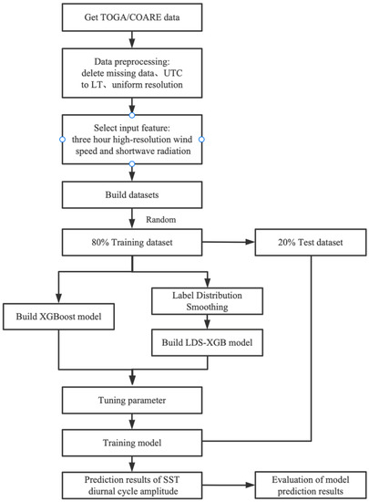
Figure 1.
Overall flow chart.
The remainder of this paper is organized as follows. The data source and preprocessing method in this study are introduced in Section 2. Section 3 presents our constructed SST diurnal cycle amplitude regression prediction model and evaluates the model’s predictive ability. Section 4 features the comparative analysis undertaken with other models. The conclusion is in Section 5.
2. Data and Pre-Processing Methods
2.1. Data Source
The observation data used are from the Tropical Ocean-Global Atmosphere Coupled Ocean-Atmosphere Response Experiment (TOGA/COARE) buoy array, including SST, wind velocity, shortwave radiation, longwave radiation, sensible heat flux, latent heat flux, etc. The data were collected from 133 stations in the range of 25° S–21° N. The temporal resolution of the data was 1 h or 10 min, and the SST diurnal cycle amplitude was obtained by calculating the difference between the maximum and minimum SST temperature every day. The data ranged from October 1992 to August 2021. The buoy distribution is shown in Figure 2.
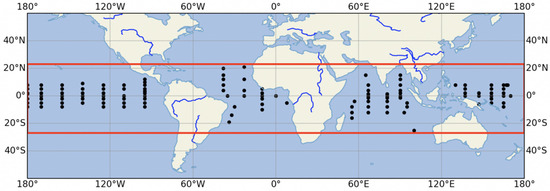
Figure 2.
TOGA/COARE buoy distribution map.
2.2. Data Pre-Processing
The main atmospheric physical parameters that affect SST diurnal cycle amplitude include shortwave radiation, longwave radiation, wind velocity, sensible heat flux, and latent heat flux [27]. Shortwave radiation and wind velocity play a more significant role than the others [27,28]. Therefore, this paper selected wind velocity and shortwave radiation as the model’s input variables. The large number of feature variables contained in the initially processed data, which may have included some less correlated features, meant that the training model would not have been able to achieve the expected prediction effect. Therefore, the feature variables with a good correlation with SST diurnal cycle amplitude were firstly selected by calculating the correlation coefficients. By calculating the correlations of daily mean wind velocity, daily mean shortwave radiation, three-hour mean wind velocity, and three-hour mean shortwave radiation with SST diurnal cycle amplitude separately, it was found that three-hour mean wind velocity and three-hour mean shortwave radiation correlated well with diurnal cycle amplitude. We also tried to use one-hour wind speed and one-hour shortwave radiation as input parameters and found that some of the input parameters were weakly correlated with SST diurnal cycle amplitude and the training time was too long. If six-hour mean wind speed and six-hour mean shortwave radiation are used as input parameters, the prediction results are not as good as the three-hour resolution. Therefore, the three-hour mean wind speed and three-hour mean shortwave radiation are selected as input parameters. The heat map of correlation coefficients between each input parameter and SST diurnal cycle amplitude is shown in Figure 3. The scale on the right side of the heat map shows the corresponding colors of the correlation coefficients. The XGBoost algorithm does not need to standardize the data because it is a tree model of border crossing and is not derivable.
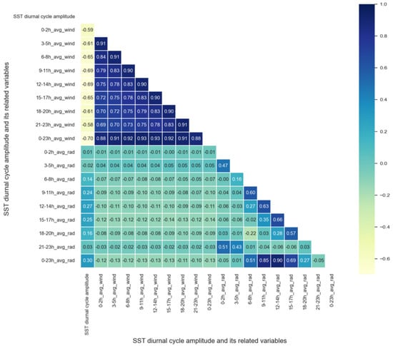
Figure 3.
Heat map of the relationship between factors related to the SST diurnal cycle amplitude.
3. Prediction Model and Analysis of Results
3.1. XGBoost Algorithm
XGBoost (extreme gradient boosting) is a machine learning algorithm based on ensemble ideas proposed by Chen et al. [29] and is essentially a gradient boosting decision tree (GBDT) that belongs to the boosting framework. Basically, the XGBoost algorithm keeps adding trees to a tree while performing feature splitting to make the tree grow to fit the residuals of the last prediction better. It rewrites and optimizes the original objective function of GBDT and executes second-order Taylor expansion to make the algorithm converge faster and obtain the optimal solution. The objective function of the XGBoost algorithm consists of two parts: one is the loss function , which is generally the mean square error, and the other part is the regularization term , which is the sum of the complexity of each tree, which is used to control the complexity of the model and prevent overfitting. Its objective function is:
where is the number of training samples, denotes the observation values of the model, denotes the simulation value of the model, denotes the number of decision trees, and denotes the kth tree model.
After the derivation by Taylor expansion, the determination of the complexity of the definition tree, and the grouping of leaf nodes, the final objective function can be written as:
Since the objective function of XGBoost algorithm can introduce a regularization term, it can control the model’s complexity, reduce its variance, and prevent it from overfitting. The XGBoost algorithm assigns learning rates to leaf nodes after each iteration to reduce the weight of each tree, reducing the impact of each tree and providing a better learning space later. The XGBoost algorithm borrows from random forests and supports column sampling, which not only reduces overfitting, but also reduces computational effort. In addition, the XGBoost algorithm also considers using multi-threading, data compression, and slicing when the amount of data is significant and memory is insufficient to improve the algorithm’s efficiency as much as possible. Therefore, the XGBoost algorithm was chosen to predict the SST diurnal cycle amplitude.
3.2. Improved XGBoost Algorithm
By calculating the probability density, the amount of observed data with an SST diurnal cycle amplitude of less than 2 °C accounted for more than 90% of the data that can be seen, while only less than 1% of the data were above 3 °C. The probability density plot is shown in Figure 4.
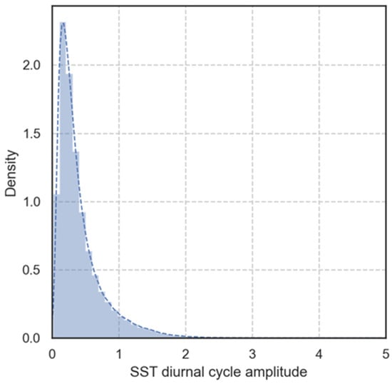
Figure 4.
Probability density plot of SST diurnal cycle amplitude.
The severe imbalance between the data led to a concentration of simulation values below 2 °C. Therefore, finding a suitable way to mitigate or solve this data imbalance problem is a critical technical challenge. Previous studies on the data imbalance problem have been based on classification problems. However, the SST diurnal cycle amplitude is continuous. In continuous data, there is no longer a rigid boundary between classes, and the direct application of traditional imbalance classification methods is not satisfactory. To address this problem, this paper used label distribution smoothing (LDS) [30] to improve the XGBoost algorithm, which predicts the SST diurnal cycle amplitude in the continuous case. The improved algorithm is called LDS-XGB and is implemented as follows.
Let denote the training set with a sample size of , where denotes the input variables, denotes the label, and is continuous. We divide the continuous type label values into groups of at equal intervals, i.e., and use to denote the group index of the target values. For predicting the SST diurnal cycle amplitude, we define .
The density distribution of the SST diurnal cycle amplitude of the labeled values in the training set, i.e., the number of occurrences of in the training set, is calculated from and is called the empirical label distribution. The Pearson correlation coefficient evaluates the linear relationship between the label density distribution and the error distribution. The larger the coefficient’s absolute value, the stronger the correlation between the two. Previous studies have shown that the empirical label density distribution does not reflect the observed label density distribution when the label values are continuous because of the dependence between data samples on adjacent labels [31]. LDS uses kernel density estimation to improve the imbalance in continuous datasets.
LDS uses a symmetric kernel function. Here, we chose to use the Gaussian kernel function . The Gaussian kernel function is a symmetric kernel function satisfying and = 0,, which portrays the similarity between the target values and . The empirical label density distribution is then convolved to obtain a new distribution, called the effective label density distribution. The calculation formula is as follows:
where represents the empirical label density distribution and represents the effective label density distribution for the label value .
In the XGboost algorithm, the regression tree loss function is generally chosen as the squared loss. After the effective density distribution is obtained by calculation, the loss function is weighted by multiplying it by the inverse of the effective density distribution of each training sample. The obtained loss function is:
where represents the reweighted loss function.
3.3. Evaluation Criteria
In the sample training process, the predictive performance of the model is evaluated using the root mean square error (RMSE), mean absolute error (MAE), and goodness of fit, . RMSE measures the deviation between the simulation values and observation values, MAE reflects the actual situation of the error in the simulation values, and demonstrates the extent to which the independent variables explain the variation in the dependent variable. These are essential yardsticks for evaluating models in machine learning. The RMSE, MAE, and are calculated as follows:
where is the observation value of SST diurnal cycle amplitude data, is the simulation value of the SST diurnal cycle amplitude, and is the number of samples.
3.4. Model Tuning
The prediction performance of a machine learning model mainly depends on the data quality and the model parameters’ tuning. Therefore, in this study, to further improve the model prediction effect, the SST diurnal cycle amplitude prediction model based on the XGBoost algorithm needed to be tuned.
Five key parameters have a significant impact on the prediction performance of the XGBoost model. Among them, n_estimators are the number of weak learners in the ensemble algorithm—the larger the value of this parameter, the stronger the learning ability of the model, but the more likely the model is to overfit; max_depth controls the maximum depth of the tree in the model—the larger the value of this parameter, the more complex the model is, and the easier it is to overfit the model; the subsample parameter controls the proportion of randomly selected data for training, and the learning_rate parameter controls the iteration rate, both of which can prevent model overfitting; and gamma controls the minimum loss function required to split the nodes, which can reduce the complexity of the model and speed up the algorithm’s convergence. We adjusted the critical parameters of the XGBoost algorithm through several rounds of testing and used the cross-validation results as the criteria for parameter selection. The final optimal values of the five key parameters are shown in Table 1.

Table 1.
Optimal values of key model parameters.
3.5. Analysis of Results
First, the observed data set, containing SST diurnal cycle amplitude, high-resolution wind velocity, and short-wave radiation values, was randomly divided into a training set and a testing set according to the ratio of 80%:20%. Second, based on the LDS-XGB algorithm, the model was trained using the training set to build a regression prediction model of the SST diurnal cycle amplitude. Finally, the model’s prediction ability was verified using the testing set. This study used the Python language environment to build the XGBoost model, mainly based on the scikit-learn library. According to the prediction algorithm flow, the pre-processed dataset was imported into the LDS-XGB model. After finding the optimal parameters, the model was trained, and the prediction results were obtained.
The Pearson correlation coefficient between the empirical label density distribution and the error distribution was first calculated (Figure 5a,c), which was −0.38, and the correlation between the empirical label density and the error distribution was weak. The effective label density distribution was obtained by Gaussian convolution of the empirical label density distribution. The Pearson correlation coefficient between the effective label density and the error distribution was −0.54. The results indicate that the effective label density distribution calculated by the LDS-XGB model had a good correlation with the error distribution (Figure 5b,d).
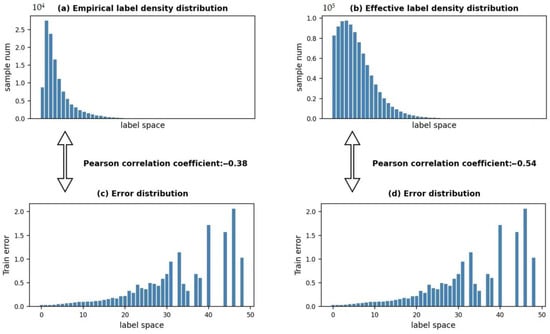
Figure 5.
Empirical label density distribution with error distribution Pearson correlation coefficient of −0.38 (a,c) and effective label density with error distribution Pearson correlation coefficient of −0.54 (b,d).
The training set was trained using the XGBoost and LDS-XGB models, respectively, and the testing set was predicted using the trained models. The prediction results are shown in Figure 6a,b, respectively, where the bottom histogram indicates the distribution of the observed data, and the right histogram indicates the distribution of the predicted data. The horizontal coordinates in the scatterplot indicate the observation values, the vertical coordinates indicate the simulation values, and the simulation values and the observation values fall on the diagonal line. Both models predicted the SST diurnal cycle amplitude better than the earlier prediction model. Table 2 and Table 3 show that both models achieved a high fit and small error values in both the training and testing sets, which proves that the models had good performance in predicting SST diurnal cycle amplitude. In terms of fit, the XGBoost model and the LDS-XGB model both achieved more than 70%. In terms of error, the RMSE values of the two models were 0.1757 °C and 0.1771 °C, respectively, with both committing minor mistakes. After statistical analysis, it was found that the proportion of SST diurnal cycle amplitude values above 2 °C predicted by the XGBoost model was less than 0.020%. In comparison, the ratio of values above 2 °C predicted by the LDS-XGB model improved to 0.28%, which was closer to the observation, indicating that the models improved the data imbalance problem to some extent and thus improved their prediction of high values.
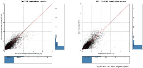
Figure 6.
XGB prediction results: (a) LDS-XGB prediction results; (b) where the bottom histogram indicates the distribution of observed data, the right histogram indicates the distribution of predicted data, the horizontal coordinates in the scatter plot indicate the observation values, and the vertical coordinates indicate the simulation values.

Table 2.
Evaluation results of SST diurnal cycle amplitude prediction model.

Table 3.
Statistics of prediction results of SST diurnal cycle amplitude model.
We also constructed three different models for the tropical Pacific Ocean, Atlantic Ocean, and the Indian Ocean, and four different models for four seasons the same as the previous. Table 4 and Table 5 evaluated the training and testing results for each model, and the results show that models do not differ significantly in prediction accuracy. Although the SST diurnal cycle amplitude behaves differently over each ocean and season, the key factors that control the SST diurnal cycle amplitude, such as wind and shortwave radiation, are consistent. Our algorithm can capture the main factors causing the SST diurnal variation amplitude and can predict the SST diurnal variation amplitude better.

Table 4.
Different oceans’ evaluation results of the SST diurnal cycle amplitude.

Table 5.
Different seasons’ evaluation results of the SST diurnal cycle amplitude.
4. Discussion
To further demonstrate the accuracy of the LDS-XGB model in predicting the SST diurnal cycle amplitude, we also compared it with empirical models and various other machine learning models. Webster et al. [7] proposed a widely used regression equation for determining the SST diurnal cycle amplitude based on the analysis of many observations. Kawai and Kawamura [6] improved the equation proposed by Webster et al. by using buoy data from tropical and mid-latitude regions (Equation (9)).
where a, b, c, and d are the regression coefficients, PS is the shortwave radiation maximum, and U is the average daily wind velocity.
We built an empirical model based on the parameters given in the paper and predicted the testing data, and the results showed prediction error and poor goodness of fit. Therefore, we used least squares to rederive the parameters based on the training data to build a new empirical model and predict the testing data. The original parameters given in the paper and the parameters obtained by least squares are shown in Table 6 and Table 7.

Table 6.
Regression coefficients (Kawai and Kawamura, 2002 [6]).

Table 7.
Least squares regression coefficients.
In addition, common regression algorithms used in machine learning, besides the XGBoost model, include the RBF (radial basis function), random forest, and stacking models. Therefore, to select the optimal model, we also tested these models to predict SST diurnal cycle amplitude data and evaluated and compared the results.
The RBF neural network is a three-layer neural network, including an input layer, a hidden layer, and an output layer. The transformation from the input space to the space of the hidden layer is nonlinear, while the transformation from the space of the hidden layer to the space of the output layer is linear. RBF [32] neural networks are simple in structure, concise in training, fast in learning convergence, and capable of approximating arbitrary nonlinear functions. Random forest is an integrated algorithm of the bagging type, which makes the overall model result in high accuracy and generalization performance by combining multiple weak classifiers. The random forest regression model consists of multiple regression trees, and there is no correlation between each decision tree in the forest; the final output of the model is determined by each decision tree in the forest together, i.e., the average of all the decision tree outputs. This makes random forests a powerful modeling technique that is much more powerful than individual decision trees. Stacking [33] is an integrated learning method that obtains a better result by combining the output generated by multiple weak learners as the input to the final learner. In the Stacking method, there are two stages of models. The first stage of the model is the model with the original training set as input, called the base model. The second stage of the model is a model with the predictions of the base model on the original training set as the training set and the predictions of the base model on the original test set as the test set, called the meta-model. XGBoost, bagging, and random forest are chosen for the base model, and simple linear regression is chosen for the meta-model to prevent overfitting.
Table 8 shows the evaluation of all models’ training and testing results. As can be seen from the table, the empirical model prediction results had the most significant error, with the MAE and RMSE reaching 53.36% and 70.96%, respectively. The MAE and RMSE were effectively reduced after the parameters were substituted into the empirical model using the least squares method. Further, the predicted SST diurnal cycle amplitude results using the three deep learning models were more accurate. The performance of the RBF neural network model was more stable on the training and testing sets, with the MAE and RMSE reduced to 10.48% and 17.73%, respectively, while the random forest results showed large fluctuations. Still, the error was significantly reduced compared to the empirical model. Stacking was more stable on the testing set, with the MAE and RMSE reduced to 11.12% and 17.44%, respectively. In terms of the goodness of fit, the of the random forest on the training set was too large, reaching 96.18%. The random forest prediction results fluctuated widely, indicating that the model was overfitted. In the testing set, the values of the random forest, stacking, and RBF neural network models increased compared to the LDS-XGB model, but only by 1~2%. Regarding the error, the RMSE of all three models was 0.17 °C, which was not much different from that of the LDS-XGB model. According to the results, the predicted SST diurnal cycle amplitude values by the empirical model and the three deep learning models were all below 2 °C, and it was almost impossible for these models to predict the values above 2 °C, which was very unsatisfactory for the high values (Table 9). In terms of algorithm, we built the XGBoost algorithm to perform a second-order Taylor expansion on the loss function. And the introduction of second-order derivatives in the XGBoost algorithm increased the accuracy to a certain extent. The regular term reduces the model’s variance and simplifies the learned model, which helps prevent overfitting. The XGBoost algorithm borrows from the random forest and supports column sampling, which not only reduces overfitting, but also reduces computational effort. Also, we used the LDS method to improve the weights of the loss function and to increase the predictive power for high values. In summary, our established LDS-XGB model effectively improves the data imbalance problem without losing prediction accuracy, improves the model’s prediction ability for high values, and achieves accurate and efficient SST diurnal cycle amplitude prediction.

Table 8.
Training and testing evaluation results for each model.

Table 9.
Statistics of prediction results for the SST diurnal cycle amplitude model.
5. Conclusions
In this study, the prediction of the SST diurnal cycle amplitude was carried out based on TOGA/COARE buoy data by building a regression prediction model using machine deep learning methods. Firstly, a regression model for predicting SST diurnal cycle amplitude was constructed using the XGBoost algorithm, and the algorithm’s effectiveness was verified by using TOGA/COARE buoy data as an example. Secondly, to solve the data imbalance problem, the LDS method was used to reweight the XGBoost model, and the LDS-XGB model was constructed, which showed a significantly improved ability to predict high values of SST diurnal cycle amplitude (greater than 2 °C). We also compared the SST diurnal cycle amplitudes in different oceans and seasons, and the results showed that the models did not differ significantly in prediction accuracy. After comparing the LDS-XGB algorithm’s SST diurnal cycle amplitude prediction results with those of various empirical models and some machine learning algorithms, it was found that the LDS-XGB algorithm performed better in terms of error and goodness of fit.
In summary, the LDS-XGB algorithm constructed in this study can accurately predict the SST diurnal cycle amplitude. Its prediction ability for high values was greatly improved compared to earlier models, achieving an accurate and efficient SST diurnal cycle amplitude prediction. For the prediction of SST diurnal cycle amplitude values above 3 °C, we plan to conduct more in-depth research on the loss function of the LDS-XGB algorithm and are continuing to explore other methods to predict SST diurnal cycle amplitude. Moreover, the phase of the diurnal cycle is the other important feature besides amplitude. We are considering conducting studies on the SST diurnal cycle phase in the future.
Author Contributions
Methodology, visualization, analysis, and writing—original draft preparation, Y.F.; supervision, and writing—editing, Z.G.; methodology and numerical experiments’ suggestion, H.X.; validation, analysis, and writing—editing, X.Y.; conceptualization, supervision, funding acquisition, and writing—review and editing, Z.S. All authors discussed, read, edited, and approved the article. All authors have read and agreed to the published version of the manuscript.
Funding
This research was funded by the Marine S&T Fund of Shandong Province for the Pilot National Laboratory for Marine Science and Technology (Qingdao) (2022QNLM010202), National Key R&D Development Program of China (2021YFF0704002), the National Natural Science Foundation of China (nos. U1806205, 42022042, and 41821004), and the China–Korea Cooperation Project on Northwest Pacific Marine Ecosystem Simulation under Climate Change.
Institutional Review Board Statement
Not applicable.
Informed Consent Statement
Not applicable.
Data Availability Statement
The TOGA/COARE data used in this study are available at https://www.pmel.noaa.gov/tao/drupal/disdel/ (accessed on 1 October 2022).
Acknowledgments
We acknowledge the three anonymous reviewers and the editor for their constructive comments and suggestions for improving the manuscript. We want to thank “The Qingdao AI Computing Center” and the “Eco-Innovation Center” for providing inclusive computing power and technical support of MindSpore during the completion of this paper.
Conflicts of Interest
The authors declare no conflict of interest.
References
- Castro, S.L.; Wick, G.A.; Buck, J.J.H. Comparison of diurnal warming estimates from unpumped Argo data and SEVIRI satellite observations. Remote Sens. Environ. 2014, 140, 789–799. [Google Scholar] [CrossRef]
- Bernie, D.J.; Guilyardi, E.; Madec, G.; Slingo, J.M.; Woolnough, S.J.; Cole, J. Impact of resolving the diurnal cycle in an ocean–atmosphere GCM. Part 2: A diurnally coupled CGCM. Clim. Dyn. 2008, 31, 909–925. [Google Scholar] [CrossRef]
- Ham, Y.; Kug, J.S.; Kang, I.S.; Jin, F.F.; Timmermann, A. Impact of diurnal atmosphere–ocean coupling on tropical climate simulations using a coupled GCM. Clim. Dyn. 2010, 34, 905–917. [Google Scholar] [CrossRef]
- Masson, S.; Terray, P.; Madec, G.; Luo, J.J.; Yamagata, T.; Takahashi, K. Impact of intra-daily SST variability on ENSO characteristics in a coupled model. Clim. Dyn. 2012, 39, 681–707. [Google Scholar] [CrossRef]
- Tian, F.; Storch, J.V.; Hertwig, E. Impact of SST diurnal cycle on ENSO asymmetry. Clim. Dyn. 2018, 14, 2399–2411. [Google Scholar] [CrossRef]
- Kawai, Y.; Kawamura, H. Evaluation of the diurnal warming of sea surface temperature using satellite-derived marine meteorological data. J. Oceanogr. 2002, 58, 805–814. [Google Scholar] [CrossRef]
- Webster, P.; Clayson, C.A.; Curry, J.A. Clouds, radiation, and the diurnal cycle of sea surface temperature in the tropical western Pacific. J. Clim. 1996, 9, 1712–1730. [Google Scholar] [CrossRef]
- Clayson, C.A.; Weitlich, D. Variability of Tropical Diurnal Sea Surface Temperature. J. Clim. 2007, 20, 334–352. [Google Scholar] [CrossRef]
- Ling, T.; Xu, M.; Liang, X.-Z.; Wang, X.L.; Noh, Y. A multilevel ocean mixed layer model resolving the diurnal cycle: Development and validation. J. Adv. Model. Earth. Syst. 2015, 7, 1680–1692. [Google Scholar] [CrossRef]
- Large, W.G.; Caron, J.M. Diurnal cycling of sea surface temperature, salinity, and current in he CESM coupled climate model. J. Geophys. Res. Oceans 2015, 120, 3711–3729. [Google Scholar] [CrossRef]
- Bernie, D.J.; Guilyardi, E.; Madec, G.; Slingo, J.M.; Woolnough, S.J. Impact of resolving the diurnal cycle in an ocean–atmosphere GCM. Part 1: A diurnally forced OGCM. Clim. Dyn. 2007, 29, 575–590. [Google Scholar] [CrossRef]
- Bernie, D.J.; Woolnough, S.J.; Slingo, J.M.; Guilyardi, E. Modeling diurnal and intraseasonal variability of the ocean mixed layer. J. Clim. 2005, 18, 1190–1202. [Google Scholar] [CrossRef]
- Bolton, T.; Zanna, L. Applications of Deep learning to Ocean Data Inference and Subgrid Parameterization. J. Adv. Model. Earth Syst. 2018, 11, 379–399. [Google Scholar] [CrossRef]
- Brenwitz, N.D.; Brethert, C.S. Prognostic Validation of a Neural Network Unified Physics Parameterization. Geophys. Res. Lett. 2018, 45, 6289–6298. [Google Scholar] [CrossRef]
- Gao, S.; Zhao, P.; Pan, B.; Li, Y.; Zhou, M.; Xu, J.; Zhong, S.; Shi, Z. Anowcasting model for the prediction of typhoon tracks based on a long short term memory neural network. Acta Oceanol. Sin. 2018, 37, 8–12. [Google Scholar] [CrossRef]
- Ham, Y.G.; Kim, J.H.; Luo, J. Deep learning for multi-year ENSO forecasts. Nature 2019, 573, 568–572. [Google Scholar] [CrossRef]
- Jiang, G.; Xu, J.; Wei, J. A Deep learning Algorithm of Neural Network for the Parameterization of Typhoon-Ocean Feedback in Typhoon Forecast Models. Geophys. Res. Lett. 2018, 45, 3706–3716. [Google Scholar] [CrossRef]
- Mandal, S.; Prabaharan, N. Ocean wave forecasting using recurrent neural networks. Ocean. Eng. 2006, 33, 1401–1410. [Google Scholar] [CrossRef]
- Men, X.; Jiao, R.; Wang, D.; Zhao, C.; Liu, Y.; Xia, J.; Li, H.; Yan, Z.; Sun, J.; Wang, L. A temperature correction method for multi-model ensemble forecast in North China based on machine learning. Clim. Environ. Res. 2019, 24, 116–124. [Google Scholar]
- Park, M.-S.; Kim, M.; Lee, M.-I.; Im, J.; Park, S. Detection of tropical cyclone genesis via quantitative satellite ocean surface wind pattern and intensity analyses using decision trees. Remote Sens. Environ. 2016, 183, 205–214. [Google Scholar] [CrossRef]
- Reichstein, M.; Camps-Valls, G.; Stevens, B.; Jung, M.; Denzler, J.; Carvalhais, N.; Prabhat. Deep learning and process understanding for data-driven Earth system science. Nature 2019, 566, 195–204. [Google Scholar] [CrossRef] [PubMed]
- Willis, M.J.; Stosch, M. Simultaneous parameter identification and discrimination of the nonparametric structure of hybrid semi-parametric models. Comput. Chem. Eng. 2017, 104, 366–376. [Google Scholar] [CrossRef]
- Zhang, T.; Xie, F.; Xue, W.; Li, L.; Xu, H.; Wang, B. Quantification and optimization of parameter uncertainty in the grid-point atmospheric model GAMIL2. Chin. J. Geophys. 2016, 59, 465–475. [Google Scholar]
- Zhang, W.; Leung, Y.; Chan, J.C. The Analysis of Tropical Cyclone Tracks in the Western North Pacific through Data Mining. Part I; Tropical Cyclone Recurvature. J. Appl. Meteorol. Clim. 2013, 52, 1394–1416. [Google Scholar] [CrossRef]
- Xu, L.; Li, Y.; Yu, J.; Li, Q.; Shi, S. Prediction of sea surface temperature using a multiscale deep combination neural network. Remote Sens. Lett. 2020, 11, 611–619. [Google Scholar] [CrossRef]
- He, Q.; Zha, C.; Song, W.; Hao, Z.; Du, Y.; Liotta, A.; Perra, C. Improved Particle Swarm Optimization for Sea Surface Temperature Prediction. Energies 2020, 13, 1369. [Google Scholar] [CrossRef]
- Yang, X.; Song, Y.; Wei, M.; Xue, Y.; Song, Z. Different Influencing Mechanisms of Two ENSO Types on the Interannual Variation in Diurnal SST over the Niño-3 and Niño-4 Regions. J. Clim. 2022, 35, 125–139. [Google Scholar]
- Gentemann, C.L.; Minnett, P.J.; Le Borgne, P.; Merchant, C.J. Multi-satellite measurements of large diurnal warming events. Geophys. Res. Lett. 2008, 35, L22602. [Google Scholar] [CrossRef]
- Chen, T.; Guestrin, C. XGBoost: A Scalable Tree Boosting System. In Proceedings of the 22nd ACM SIGKDD International Conference on Knowledge Discovery and Data Mining, San Francisco, CA, USA, 13–17 August 2016; pp. 785–794. [Google Scholar]
- Yang, Y.; Zha, K.; Chen, Y.C.; Wang, H.; Katabi, D. Delving into Deep Imbalanced Regression. In Proceedings of the International Conference on Machine Learning, Online, 7–18 July 2021. [Google Scholar]
- Parzen, E. On the estimation of a probability density function and mode. Ann. Math. Stat. 1962, 33, 1065–1076. [Google Scholar] [CrossRef]
- Moody, J.; Darken, C. Fast Learning in Networks of Locally-Tuned Processing Units. Neural Comput. 1989, 1, 281–294. [Google Scholar] [CrossRef]
- Wolpert, D.H. Stacked generalization. Neural Netw. 1992, 5, 241–259. [Google Scholar] [CrossRef]
Publisher’s Note: MDPI stays neutral with regard to jurisdictional claims in published maps and institutional affiliations. |
© 2022 by the authors. Licensee MDPI, Basel, Switzerland. This article is an open access article distributed under the terms and conditions of the Creative Commons Attribution (CC BY) license (https://creativecommons.org/licenses/by/4.0/).