Article

Nonlinear Predictive Framework of the Undrained Clay Slope Effect on the Initial Stiffness of p-y Curves of Laterally Loaded Piles by FEM

1
School of Resources and Safety Engineering, Central South University, Changsha 410083, China
2
Hunan Provincial Key Laboratory of Hydropower Development Key Technology, Changsha 410014, China
*
Author to whom correspondence should be addressed.
J. Mar. Sci. Eng. 2022, 10(11), 1684; https://doi.org/10.3390/jmse10111684
Submission received: 20 September 2022 / Revised: 28 October 2022 / Accepted: 28 October 2022 / Published: 7 November 2022
(This article belongs to the Special Issue Advances in Marine Engineering: Geological Environment and Hazards)

Abstract

:
The hyperbolic p-y curve method is commonly used to design laterally loaded piles, in which the initial stiffness is one of the two key parameters that need to be determined. In this paper, the effect of an undrained clay slope on the initial stiffness of p-y curves of laterally loaded piles was explored, and nonlinear models of the reduction factor ( μ ) were proposed. A series of finite-element analyses was performed for different pile–slope geometric relationships according to whether the slope geometry had influence on pile–soil interaction, in which the geometrical parameters were varied. Based on simulation results, a semi-empirical method was mainly used to derive nonlinear formulations for the undrained clay slope effect on the initial stiffness of hyperbolic p-y curves. The wedge failure theory was also used to analyze the effect of the dimensionless slope height on the initial stiffness. Comparing with other researchers’ reduction factor models, the results of the present model are in the reasonable range and can predict more cases. Test cases were used to validate the proposed model, and the results show that theoretical results are in better agreement with test results using the present model.

1. Introduction

Piles have been widely used in marine geotechnical engineering to support axial and lateral loads for different structures, such as offshore wind turbines, bridges, and offshore drilling platforms constructed at or near the slope [1,2,3,4]. There are several methods to analyze the load–displacement characteristics of laterally loaded piles. The p-y curves method is known to be a relatively accurate and effective method [5,6]. Many investigators have developed p-y curves for sand [7,8,9], clay [10,11,12], and rock masses, [13,14] mainly based on laboratory tests [15,16], field tests [17], and numerical simulation [18,19,20]. A popular hyperbolic p-y curves method is commonly used to predict the load–displacement characteristics of the soil–pile system under lateral load. There are two key parameters in p-y curves, which are initial stiffness ( K i ) and ultimate resistance of the soil ( p u ) [13,21,22]. The ultimate resistance of the soil ( p u ) determines the ultimate state, and the initial stiffness ( K i ) determines the initial state for a pile under lateral load. Accurately calculating p u and K i is a crucial step to establish p-y curves, and it is meaningful in the design of laterally loaded piles.
In clayey soils, the ultimate soil resistance ( p u ) is found to increase nonlinearly with depth, and a consensus regarding how this term is evaluated is evident in the literature [18,23,24,25]. However, different formulas of the initial stiffness ( K i ) have been proposed based on the results of laboratory tests, in-situ tests, and finite-element methods. Vesic [26] proposed an elastic solution model which was deduced from the theory of a beam on an elastic Winkler foundation. Rajashree and Sitharam [5] suggested that the value of initial stiffness could be taken as twice that of Vesic’s model to account for real soil resistance around the circumference of the pile, a suggestion which was widely used by researchers. Then the model was modified to take into account the effect of diameter or depth [13,27,28,29]. These models considered the effect of different soil–pile parameters and resulted in distinct engineering performances [30]. However, these models just focus on the case of piles on level ground. When the pile is embedded in or near the slopes, the initial stiffness is decreased because of the weakening of the soil in front of the pile [22], which is rather different from that of level ground.
The slope effect on the pile–soil response often refers to the weakening effect of the slope parameters (e.g., slope angle, slope height, near-slope distance and so on) on the pile lateral load capacity. Available information concerning the clay slope effect on the initial stiffness of p-y curves is rather limited and mainly refers to linear analysis. Several investigations have considered the equivalent problem of initial stiffness of p-y curves for the case of piles in or near clay slope. Georgiadis and Georgiadis [18] performed a series of FEA simulations of piles at relatively gentle slopes, and provided a reduction factor ( μ ) which represented the linear weakening effect of the slope angle. Then Georgiadis and Georgiadis [22] provided a smooth transition from a pile at the slope crest to a pile near the slope crest. However, the equation proved to be relatively accurate only for slope angles lower than 30°. Yang et al. [16,31] performed laboratory tests and FEA simulations for a pile at the slope crest or in the slope. The results indicated that the critical depth (the depth with the initial stiffness equal to one) increased with the slope angle. A linear model of the reduction factor ( μ ) was then provided. Jiang et al. [9] provided an elastic stress solution of the soil in a slope under the self-weight, which proved to be accurate only for a narrow range of the slope angle. Considering that the current researches for the undrained clay slope effect on the initial stiffness are insufficient and have some weaknesses, systematical and comprehensive studies should be performed to explore the real slope effect on the initial stiffness of the pile–soil system.
To analyze the undrained clay slope effect on the initial stiffness, this paper established a series of 3D undrained finite-element models. Different pile–slope position relationships were considered according to whether the slope geometry had influence on pile–soil interaction. Based on simulation results, a semi-empirical method was mainly used to derive nonlinear formulations for the slope effect on the initial stiffness of hyperbolic p-y curves. The wedge failure theory was used to analyze the effect of the dimensionless slope height. Then the model performance of the present study was compared with those of other researchers’ models. Moreover, the pile head load–displacement curves and p-y curves deduced with the proposed model were validated with other test results. The new model proved to be more appropriate and reasonable to fit real cases and could predict more cases.

2. Basic Assumptions

Based on the length relationship between the pile length and the slope height, two cases are considered in this paper: the case of “no slope geometry effect” and the case of “existence of the slope geometry effect”. The case of “no slope geometry effect” refers to the slope geometry having no influence on the shape of the affected area with load increase. The case of “existence of slope geometry effect” refers to the slope geometry having influence on the shape of the affected area with load increase. The detail of the concept will be discussed in Section 4.2.1. Based on these two cases, considering the distance between the pile and slope crest, pile–slope geometry relationships can be divided into five detailed cases, as in Table 1.
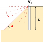
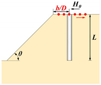
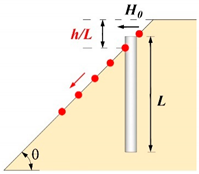
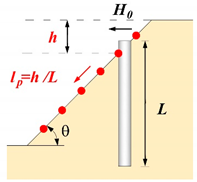
Three parameters are focused on in the “no slope geometry effect” case, which are slope angle ( θ ), dimensionless near-slope distance ( b / D ) and dimensionless pile head-crest distance ( h / L ), as seen in Table 1(a–c). Two parameters are focused on in the “existence of the slope geometry effect” case, which are dimensionless slope height ( h p ) and pile location in the slope ( l p ), as seen in Table 1(d,e).
The basic assumptions in this paper are described as follows:
(1)
The slope is stable and flat without a sliding surface, and the pile head is free.
(2)
The pile bends because of the pile head lateral load. Based on the discussions on p-y curves by Reese et al. [21] and Terzaghi [32], the soil resistance is assumed to be nonlinear with pile displacement. The popular hyperbolic p-y curve method is adopted to reflect the nonlinear response of laterally loaded piles as the following:
p = y / y / p u + 1 / K i
where p u is the ultimate lateral load per unit length, and K i is the initial stiffness.
(3)
The ultimate soil resistance ( p u ) in front of and behind the pile varies nonlinearly with depth [18,23,24,25]. The initial stiffness ( K i ) of undrained clayey soil in the level ground case is independent on depth [26,28,29].
(4)
Based on the study of Georgiadis and Georgiadis [18], a reduction factor ( μ ) is adopted to reflect the undrained clay slope effect on the initial stiffness:
μ = K i θ / K i 0
where K i θ is the initial stiffness in the slope condition, and K i 0 is the initial stiffness in the level ground condition. For the convenience of readers, this paper provides the description of some used symbols, as shown in Table 2.
(5)
Poulos’ relative stiffness ( K R ) method is used to judge whether a pile is flexible or rigid, as follows [33]:
K R = E p I p E s L 4 > 0.208                 R i g i d   p i l e < 0.0025             F l e x i b l e   p i l e
where E p I p is the bending stiffness, E s is the soil Young’s modulus, and L is the pile length. When 0.0025 K R 0.208 , the pile is not rigid or flexible, which is named elastic pile.

3. Finite-Element Analysis

The finite-element analysis program ABAQUS was used to perform analyses in which the geometrical characteristics of the problem (slope angle θ , dimensionless near-slope distance b / D , dimensionless pile head-crest distance h / L , dimensionless slope height h p , pile location in slope l p , pile length L ) were varied. Material properties were the same as Georgiadis and Georgiadis’ numerical simulation data [18], as shown in Table 3, and variable values are shown in Table 4.
The soil was modeled as a linear elastic–perfectly plastic Tresca material [34,35,36] with the undrained Young’s modulus E s = 14 MPa, the undrained shear strength c u = 70 kPa, Poisson ratio ν u = 0.49 , and the bulk unit weight γ s = 18 kN/m3. Since the loading was undrained, the limiting pile–soil adhesion τ = α s c u , where α s is adhesion factor. Considering the lower bound of the relationship between α s and c u , α s was calculated to be 0.5 for the contact between the pile and soil, according to Georgiadis and Georgiadis’ study [18]. The breadth and the bottom depth of the FE model were set to be ten times and six times the pile diameter, respectively, which is enough to eliminate the boundary effects [37,38].
All piles were modeled with a diameter ( D ) of 1 m. The piles were assumed to behave in a linear elastic manner [18,36], with Young’s modulus E p = 2.9 × 10 7 kPa, Poisson’s ratio υ = 0.1 , and the bulk unit weight γ p = 25 kN/m3. Piles were modeled with lengths of L = 4 m, 12 m, and 20 m. The relative stiffness ( K R ) of the three length piles are calculated in Equation (3) to be 0.3972, 0.0050, and 0.0006, respectively. Thus, the three piles can be regarded as rigid pile, elastic pile, and flexible pile, respectively.
More than 80 models were established in the present study. A typical 3D finite-element meshing of the 30 ° slope soil is shown in Figure 1. Eight-node quadrilateral (C3D8R) interface elements were used for the majority part of both the pile and the soil. There was more detailed meshing around the pile to allow effective pile–soil separating at the back of the pile. In this method, the total element number of models was around 8000 to 20,000. Each analysis step was performed referring to the construction process of drilled piles. The simulation could be divided into five construction parts. First of all, the bottom boundary of the mesh was fixed in all directions, and other boundaries were fixed only in the normal direction. Secondly, the geostatic equilibrium of soil domain under self-weight was considered without the pile. Thirdly, the soil elements located at pile positions were removed and the pile elements were activated. The normal and tangential contact between pile and soil were applied. Fourthly, self-weight was applied on the pile through gravity loading, and the overall model was balanced again. Finally, the lateral load was applied on the top of the pile and the response of the pile was analyzed. Note that each load increment was 100 kN for 12 m and 20 m piles and 20 kN for 4 m piles. For the case of θ = 90 ° , all boundary conditions would work at first to balance the crustal stress, and then the boundary near the pile-placed side would be removed to form a 90 ° slope. It is noted that large angles like 75° and 90° are rare in engineering, and are just used to explore the real slope effect on the initial stiffness in this paper.
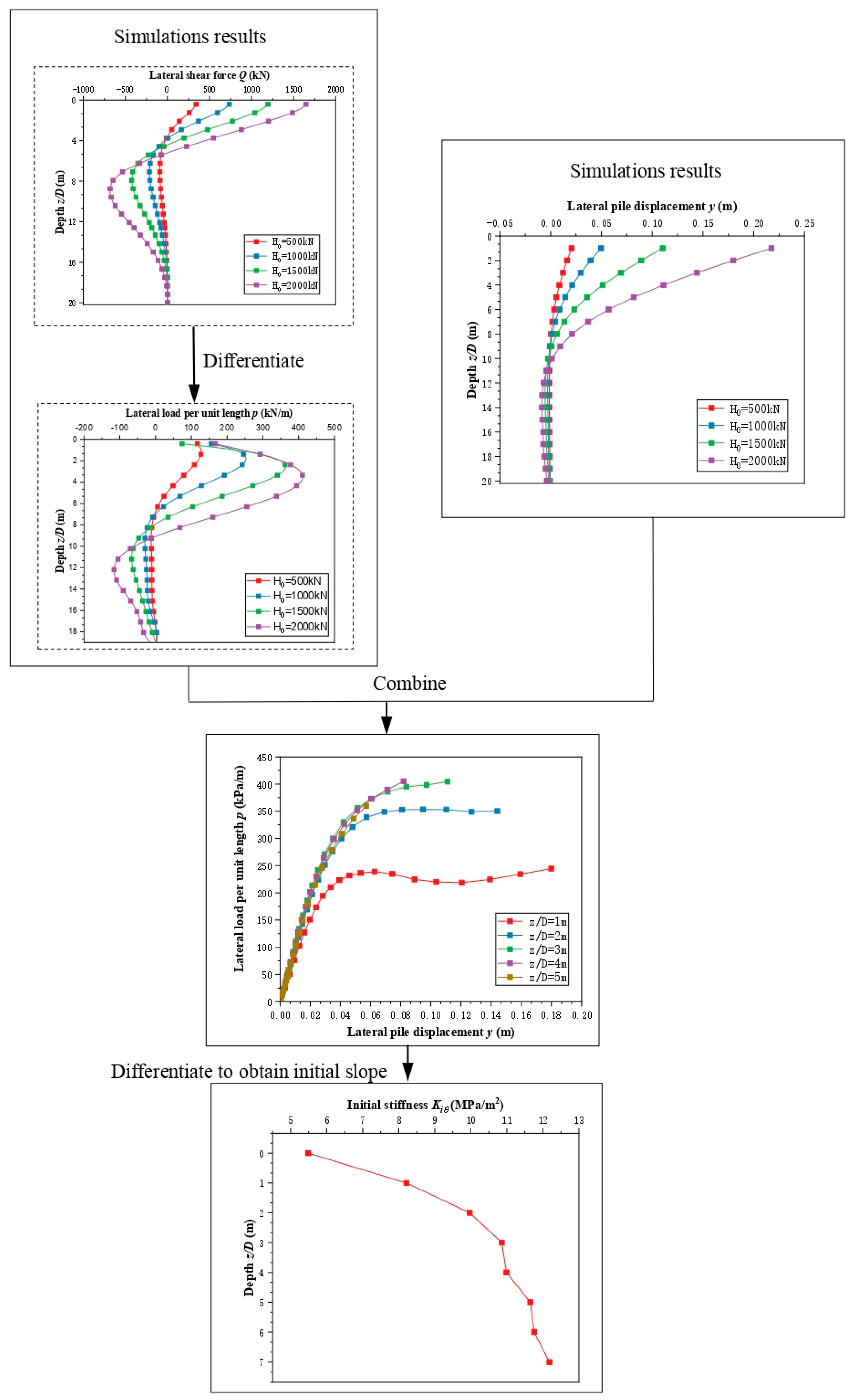
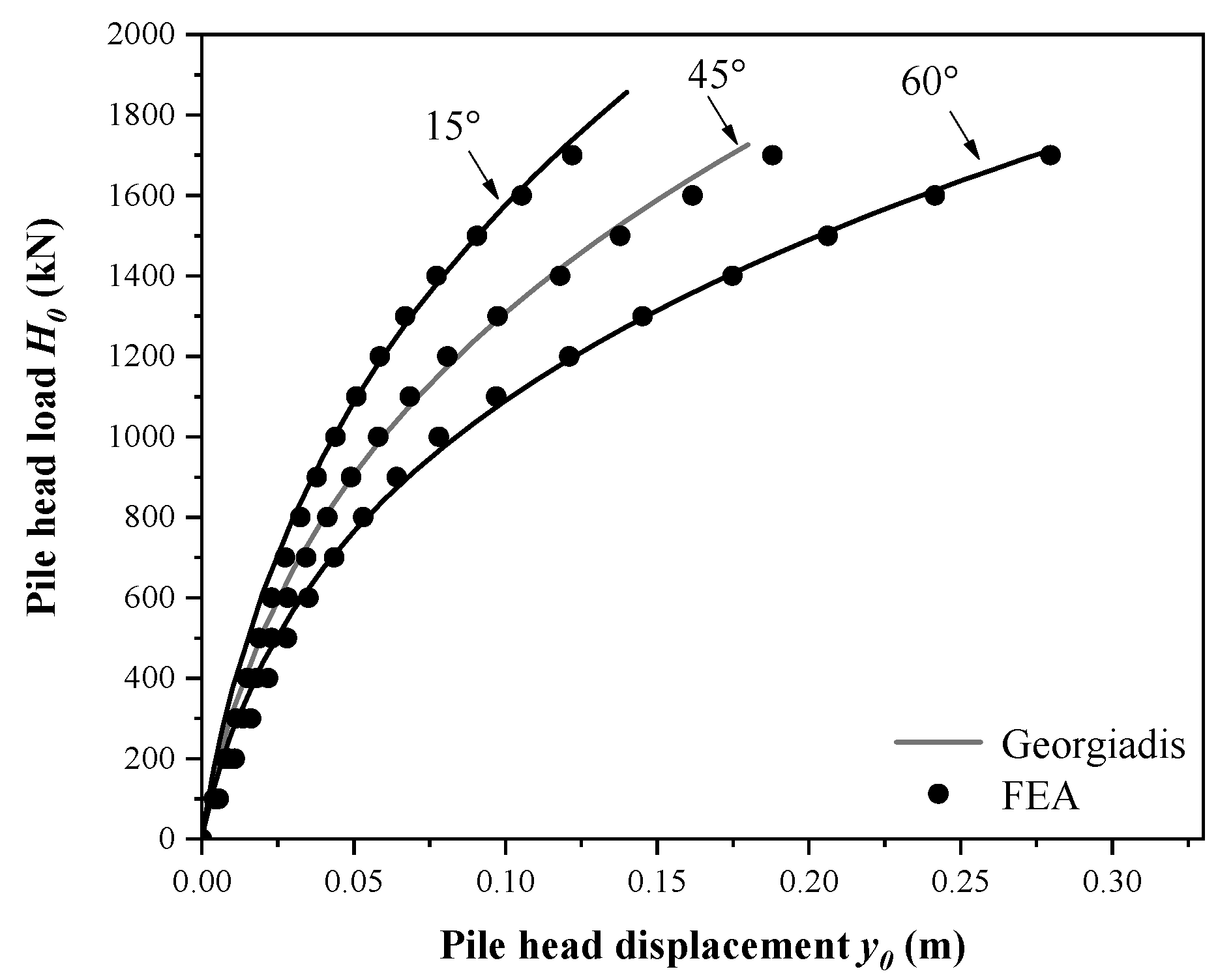
Figure 2 shows the comparison between FEA results and the theoretical method of Georgiadis and Georgiadis [18]. The pile length is 20 m, the slope angles are 15°, 45°, and 60°, and the other parameters are the same as shown in Table 1. The results prove that the FEA results are within the reasonable range. To derive p-y curves, the curves of shear force ( Q ) versus depth ( z ) were exported from the nodes of the piles of FEA results. The Q-z curves were curve-fitted in a relatively accurate method of seven-order polynominal function. Then the polynominal functions were differentiated to give curves of lateral load per unit pile length ( p ) and depth ( z ) for each pile head lateral load. The obtained p-z curves were combined with y-z curves to produce p-y curves. Then, the initial slopes of these p-y curves could be obtained as the initial stiffness ( K i ). Then, the reduction factors ( μ ) could be obtained using Equation (2). The whole procedure is shown in Appendix B. The total number of data on the initial stiffness was around 700.
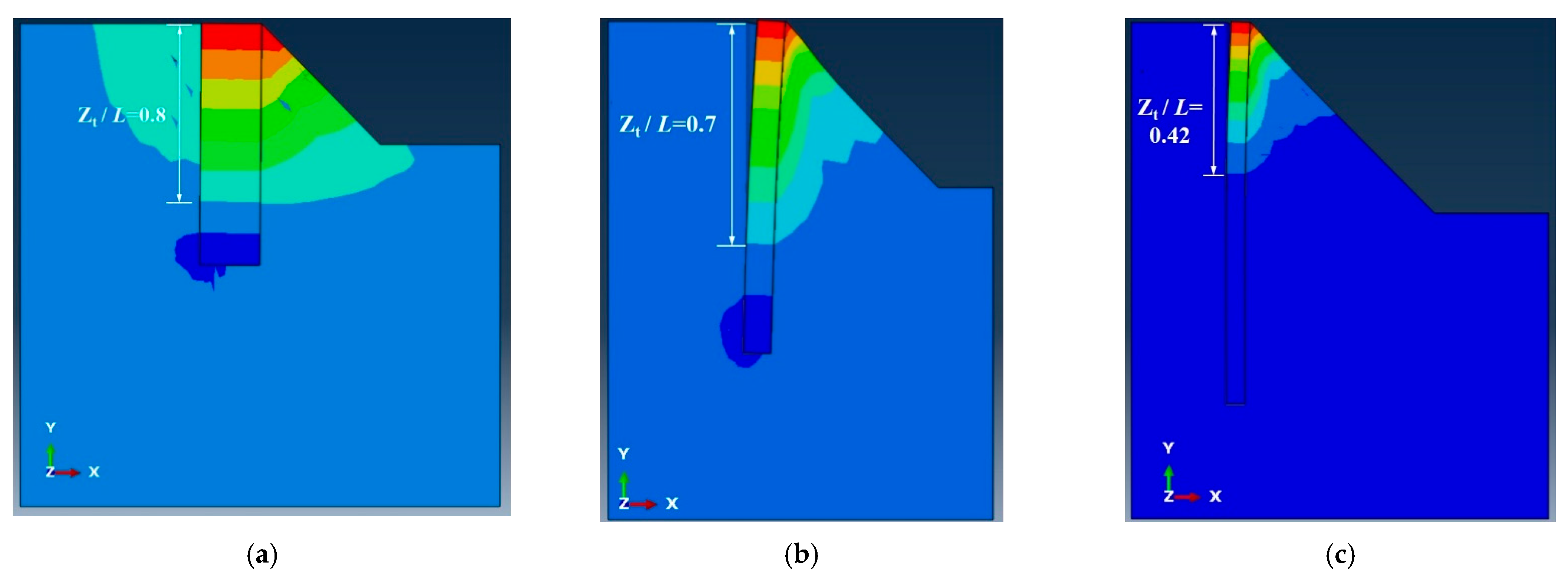
Note that the used polynomial method may have resulted in discontinuity at the ground surface and pile end. Thus, the data on fitting results at ground surface were invalid and not used in the present study. Moreover, the data of the nodes below the first turning point were not considered (e.g., as shown in Figure 3a, though the pile length is 20 m, only the data for the depths from 1 m to 7 m are used, because the pile first turns at around the depth of 8 m).

4. Theoretical Analysis for FEA Results

Based on cases with different slope heights, the pile–slope geometry relationships can be divided into two main cases, as Table 1 shows: (1) the “no slope geometry effect” case and (2) the “existence of the slope geometry effect” case. The following sub-sections will discuss the slope effect on the initial stiffness based on these two cases.

4.1. The “No Slope Geometry Effect” Case

In this case, three parameters are focused on, which are slope angle ( θ ), dimensionless near-slope distance ( b / D ), and dimensionless pile head-crest distance ( h / L ), as seen in Table 1(a–c). Theoretical analyses about the effect of these parameters are discussed in the following sub-sections, based on FEA simulation results.

4.1.1. Case 1: Variation of Slope Angle ( θ )

In this case, the pile is installed at the crest, as seen in Table 1(a). The reduction factor ( μ θ ) is calculated as shown in Figure 3. Different from the linear results of Georgiadis and Georgiadis [18] and Yang et al. [30], the reduction factor ( μ θ ) increases nonlinearly with the depth in this paper. These nonlinear curves indicate that the value of the initial stiffness ( K i θ ) in slope conditions approaches K i 0 with depth. The empirical exponential equation is provided as following:
μ θ = K i θ K i 0 = cos a θ + 1 e β z / D cos θ 1 cos a θ
where α and β are non-dimensional coefficients, which are determined in Section 4.1.2. Equation (4) shows that the reduction factor ( μ θ ) increases from cos a θ at horizontal ground ( z = 0 ) and nonlinearly approaches 1 with the depth ( z ).

4.1.2. Case 2: Variation of Dimensionless Near-Slope Distance ( b / D )

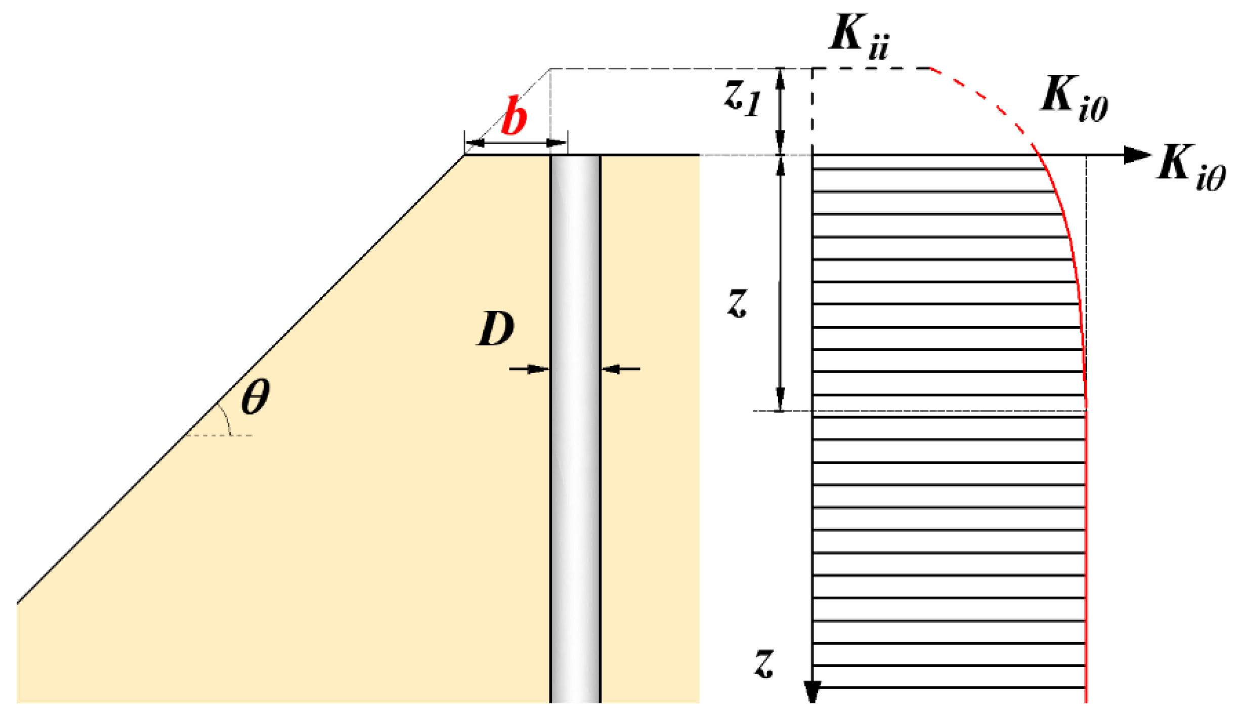
In this case, the pile is installed at a distance ( b ) from the slope crest, as seen in Table 1(b). Considering the effect of the near-slope distance, an idealization is illustrated in Figure 4, where K ii is the value of the initial stiffness at depth z = 0 at horizontal ground. It provides a smooth translation from a pile at the slope crest to one near the slope. By replacing depth ( z ) in Equation (4) with z + z 1 , where z 1 = b D / 2 tan θ , it becomes:
μ b / D = K i θ K i 0 = cos a θ + ( 1 e β z + b 0.5 D tan θ cos θ / D ) 1 cos a θ
Equation (5) can also be expressed as follows:
μ b / D = K i θ K i 0 = cos a θ + ( 1 e β z cos θ + b 0.5 D sin θ / D ) 1 cos a θ
In the ideal case of θ = 90 ° at the slope crest, there is no Winkler spring in the outside part of the pile, so K i θ = 0 and μ b / D = 0 . When a pile is not installed at the slope crest, there is still soil constraining the outside of the pile. In this case, Equation (6) becomes:
μ b / D = 1 e β b / D 0.5
Equation (7) demonstrates that for the ideal case of θ = 90 ° , the slope has the same effect on K i θ at any depth, and K i θ just changes with the distance ( b ). Then, the parameter β in Equation (7) can be determined through a series of b / D effect simulations in the case of θ = 90 ° .
Figure 5 shows results of the slope angle ( θ ) effect on μ b / D by deriving the results from FEA. Averaging the results to obtain the ratio of slope case to level ground case, μ b / D becomes 0.32, 0.46, 0.62, 0.74, 0.81, and 0.88, respectively. Then, substituting μ b / D values into Equation (7), β is obtained as 0.39, 0.42, 0.39, 0.38, 0.37, and 0.38, respectively. Thus, β = 0.4 is suggested to be reasonable for use in this study.
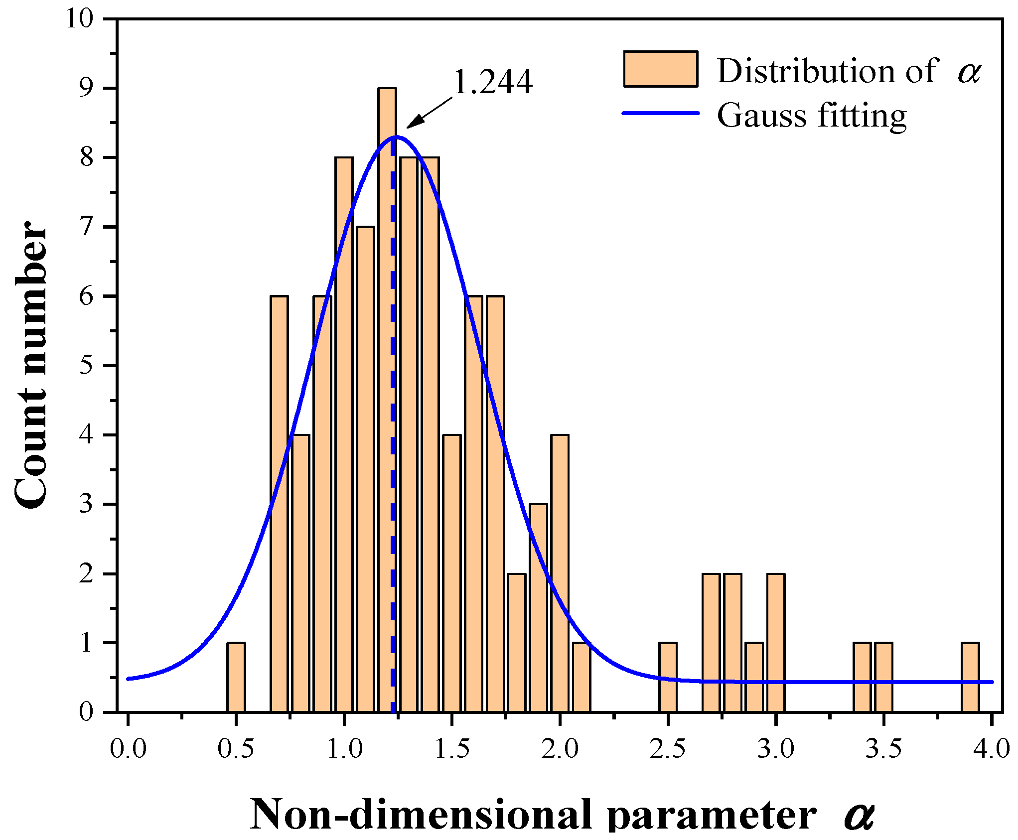
Since β is determined, α can be determined in Equation (6) by fitting curves in Figure 3. Figure 6 shows the distribution of α for a total of 95 data from piles. Then, a recommended value of α = 1.2 . is able to represent the most cases precisely.
Finally, now that α = 1.2 and β = 0.4 have been obtained, Equation (6) can be provided as:
μ b / D = K i θ K i 0 = cos 1.2 θ + 1 e 0.4 z cos θ + b 0.5 D sin θ / D 1 cos 1.2 θ
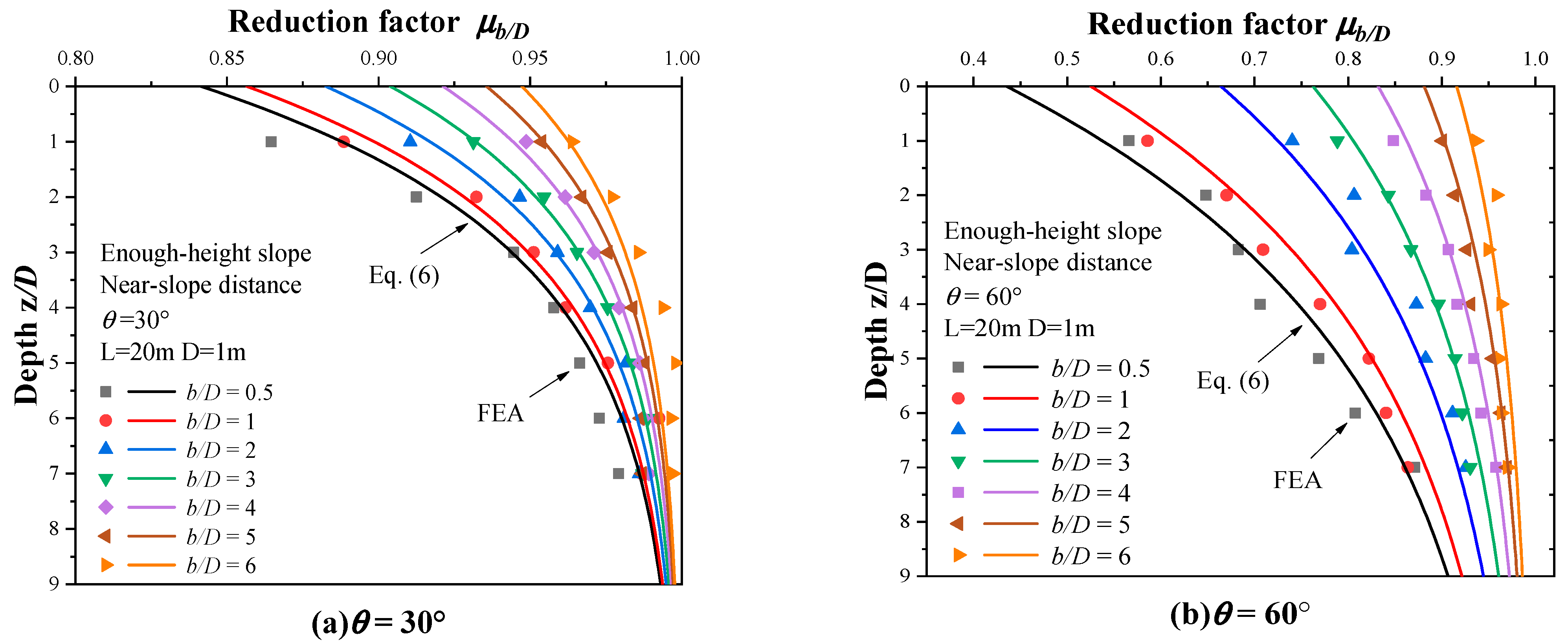
Additional cases of both the dimensionless near-slope distance ( b / D ) and the slope angle ( θ ) effects are conducted using FEA, and the results of μ are plotted in Figure 7, together with curves of Equation (8), which shows good agreement between predictions and simulation results.

4.1.3. Case 3: Variation of Dimensionless Pile Head-Crest Distance ( h / L )

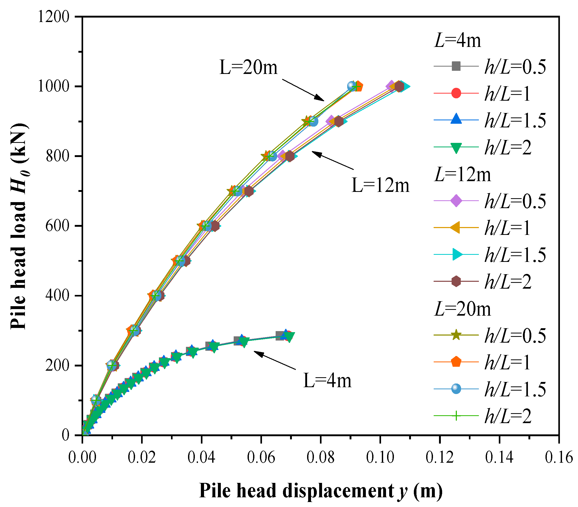
In this case, the pile is installed on the slope, at a distance h away from the slope crest, as seen in Table 1(c). As shown in Figure 8, the lateral bearing capacity is almost independent of the pile head-crest distance ( h ). This phenomenon indicates that the soil behind the pile hardly participates in the soil–pile response for undrained clay slopes, which is similar to the results of Sivapriya et al.’s laboratory test [39]. This can be explained by the theory of Coulomb earth pressure, which considers that the active earth pressure is dependent on the soil properties and the height of the structure. Thus, the case of the variation of dimensionless pile head-crest distance ( h / L ) is nearly the same as that of the pile at the slope crest. The slope effect on the initial stiffness in this case can be expressed as:
μ h / L = μ θ

4.2. The “Existence of the Slope Geometry Effect” Case

In this case, two parameters are focused on, which are dimensionless slope height ( h p ) and pile location in slope ( l p ), as seen in Table 1(d,e). Theoretical analyses about these parameters are discussed in the following sub-sections, based on simulation results.

4.2.1. Case 4: Variation of Dimensionless Slope Height ( h p )

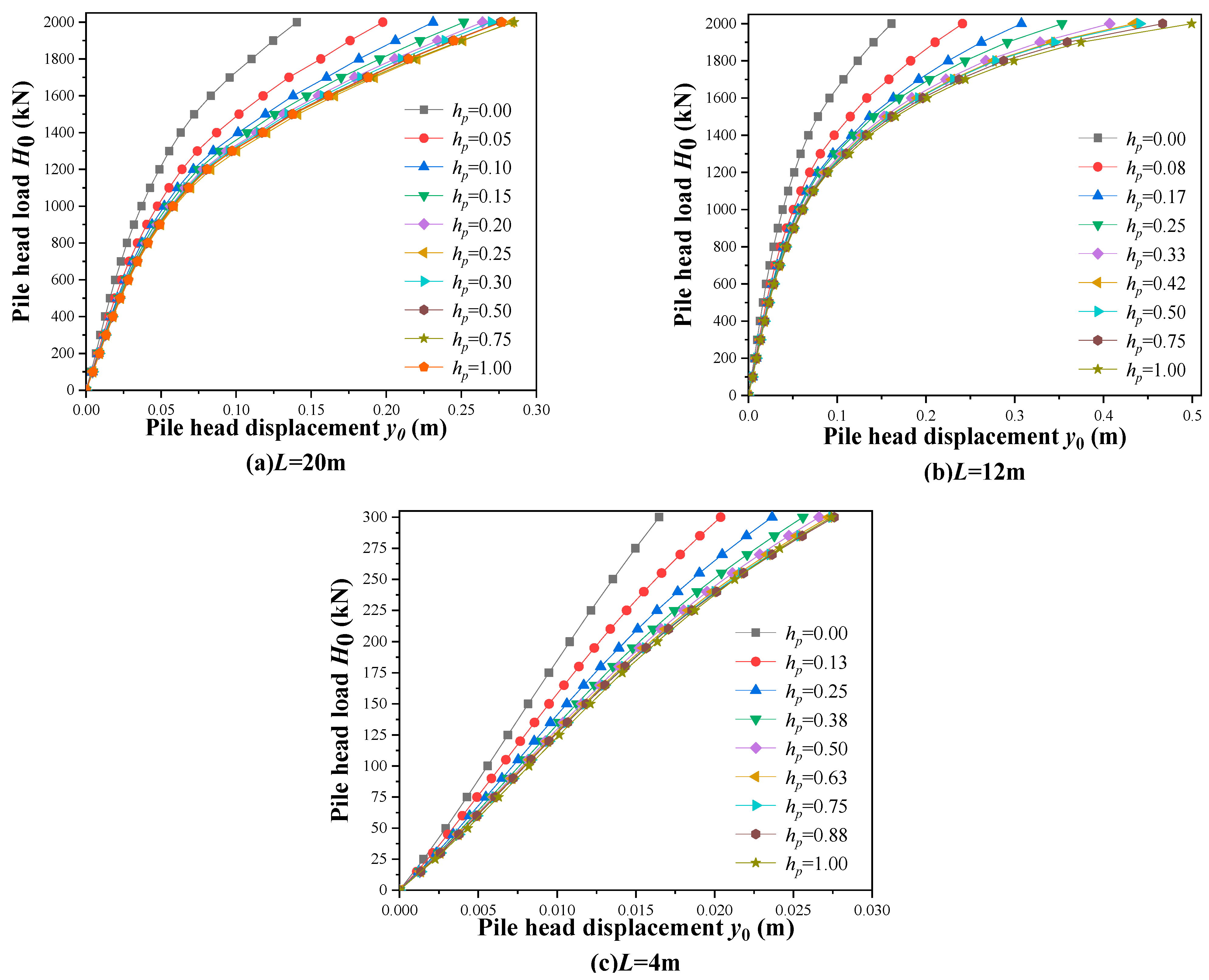
In this case, the pile is installed at the crest and dimensionless slope height ( h p ) varies, as seen in Table 1(d). Figure 9 shows that the lateral bearing capacity decreases with the increase of h p from 0 to 1 for slope angle θ = 45 ° . It is obvious that h p hardly affects the soil–pile response when h p is beyond a certain height (e.g., the curves in Figure 9a when h p 0.30 ). This indicates that the dimensionless slope height ( h p ) affects the soil–pile response in a nonlinear way.
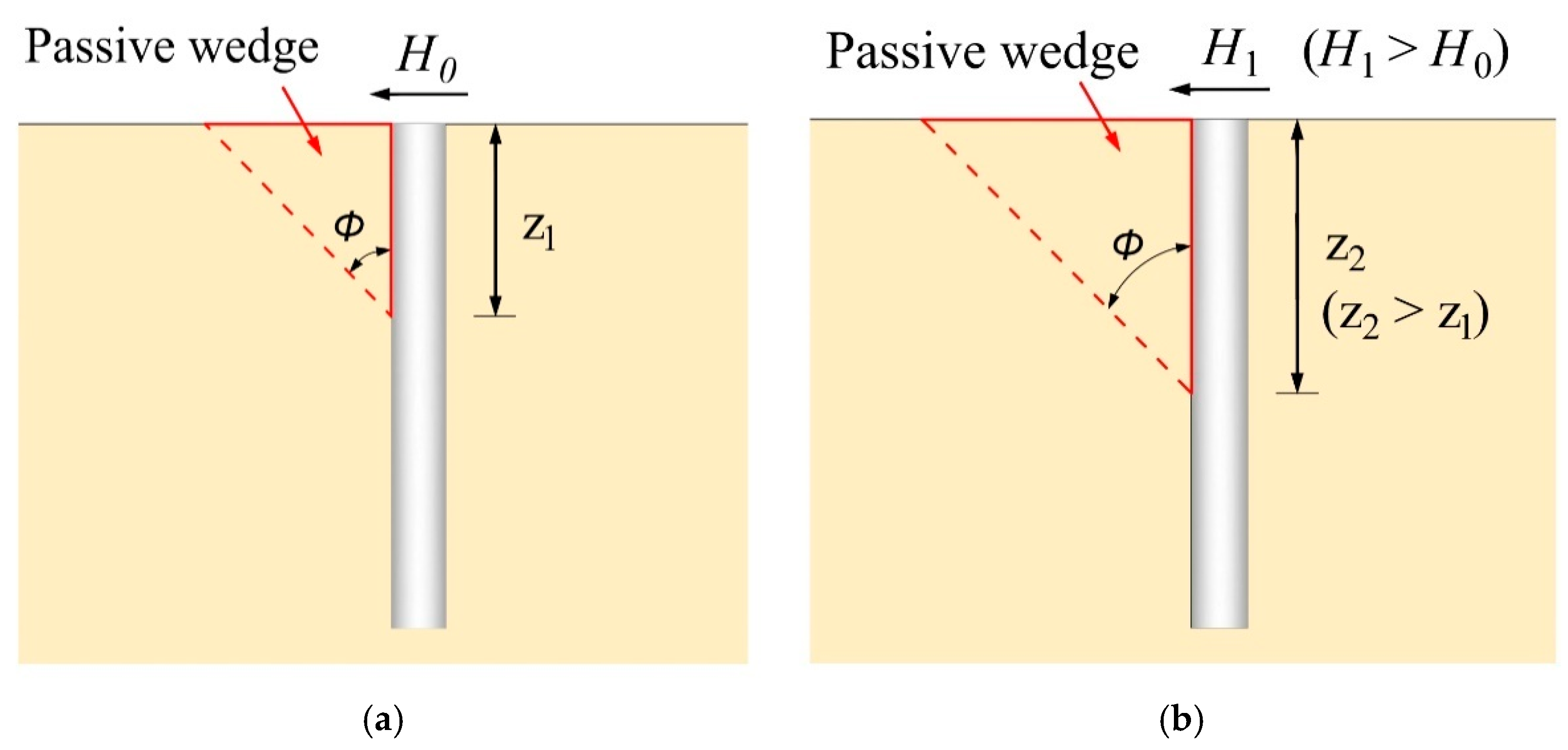
The phenomenon can be explained by a wedge failure theory first proposed by Reese and Welch and Reese et al. [40,41]. The wedge failure model considers that the soil–pile response relates to the lowest value of two possible failure mechanisms: a wedge failure mechanism at shallow depths and a flow failure around the pile at greater depths. Moreover, the passive wedge develops along the depth as the load increases to form a larger wedge failure body, as shown in Figure 10, where ϕ is the angle between the sliding surface and the vertical plane. Under undrained conditions, the angle ( ϕ ) is suggested to be 45 ° by Reese et al. [41].
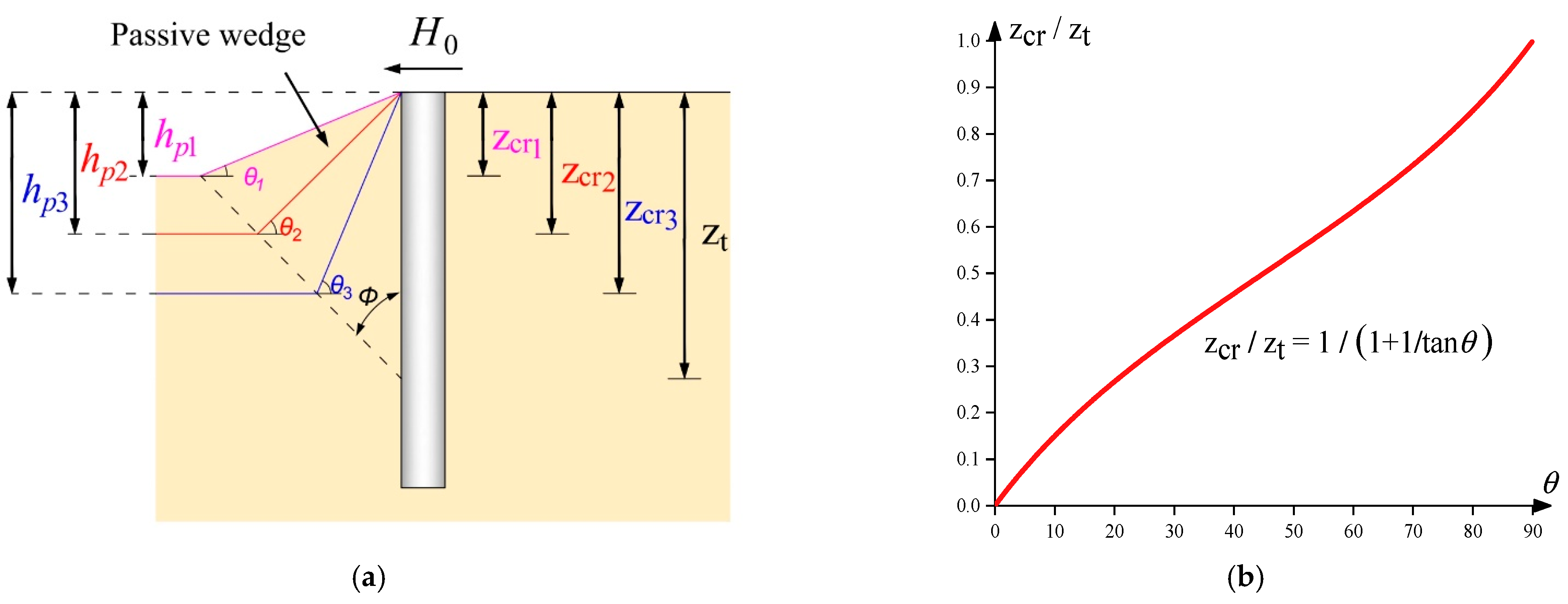
Yang et al. analyzed the near-slope failure wedge for three “existence of the slope geometry effect” cases. The study considered that as the load increased, the passive wedge expanded, and the passive wedge shape changed from a triangle to a concave quadrilateral [31]. However, a theoretical largest passive wedge exists because the depth of the bottom of the wedge will not exceed the first bending point of the pile. Similarly, for the changing h p case in this paper, the shape of the largest passive failure wedge changes from a concave quadrilateral for a small h p value to a triangle for a larger h p value, as shown in Figure 11, where z t is the depth of the first turning point, and z cr is the depth of the intersection of the bottom plane of the largest passive wedge and the slope surface.
For “existence of the slope geometry effect” cases, when the slope angle remains constant, the shape of the theoretical largest passive wedge changes with h p when h p < z cr / L , but remains constant when h p z cr / L , as shown in Figure 11. This indicates that “existence of the slope geometry effect” cases are the same as “no slope geometry effect” cases when h p z cr / L . The reduction factor ( μ h p ) can be calculated for the dimensionless slope height ( h p ) variation case as follows:
μ h p = f h p , μ θ , h p < z cr / L μ θ , h p z cr / L
where z cr is related to the slope angle, as shown in Figure 12, and can be calculated in geometry as follows:
z cr = z t / ( 1 + 1 tan θ )

Calculation Method of z t

Actually, the depth of the first turning point ( z t ) of the pile is dependent on soil and pile properties, loading conditions, and so on (e.g., for a certain pile, the value of z t approaches 0 when the soil stiffness is extremely large, but approaches the value of L when the soil stiffness is extremely small). Sun et al. [36] also indicated this, providing a range of 0.62 ~ 0.73 L for z t of a large-diameter monopile on sandy level ground. In this paper, the variation of z t is considered to be related to the relative stiffness ( K R ). It is obvious that the relative stiffness ( K R ) is influenced by the pile length because of the fourth order of the pile length ( L ) in Equation (3). Recording the depths of the first turning point ( z t ) of piles derived from FEA results, as shown in Figure 13, the ratio ( z t / L ) results of the depth of the first turning point and the pile length are shown in Figure 14. The figure indicates that z t / L decreases as the pile length increases. For each length of the undrained, laterally loaded pile, z t / L remains almost the same value.
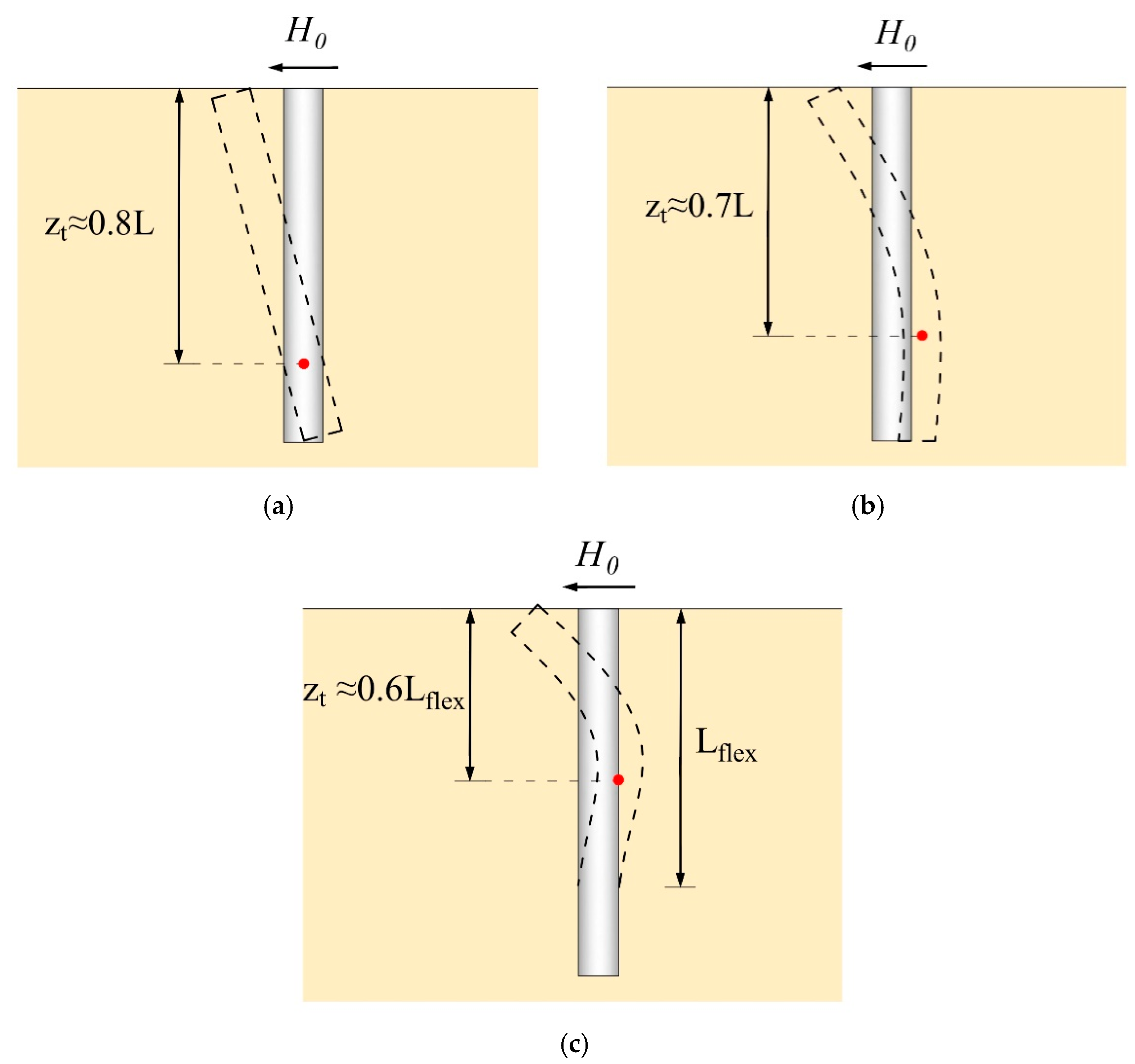
However, when the pile is flexible, the lower part of the pile hardly bears the load. As a result, z t does not increase with the pile length. Thus, the value of z t / L is around 0.7 for 4 m and 12 m length piles, but is as small as 0.4 for 20 m length piles, as shown in Figure 14. To solve the problem, a minimum flexible pile length ( L flex ) is proposed in this paper, which can be calculated with Equation (3) when K R = 0.0025, as follows:
L flex = E p I p 0.0025 E s 4
The minimum flexible pile length ( L flex ) for the pile and soil in this paper is calculated to be 14.28 m (0.71 L ). This means that when the pile is longer than 14.28 m, the lower part of the pile will not bear the load, and z t will not increase with depth. Thus, in this case, L flex and z t are considered to be unchanged for the flexible pile. Then, for the flexible pile with a length of 20 m in this paper, z t = 0.4 L ( 0.56 L flex ) is finally obtained. The variation of z t can be regarded as 0.8 L ~ 0.6 L flex for a pile varied from rigidity to flexibility, as shown in Figure 15.
A simple calculation method of z t is provided in this paper, as seen in Equation (13). Further discussions of z t can be studied by researchers in the future.
z t = 0.8 L                         Rigid   pile 0.7 L                         Elastic   pile 0.6 L flex               Flexible   pile

Calculation Method of f h p , μ θ

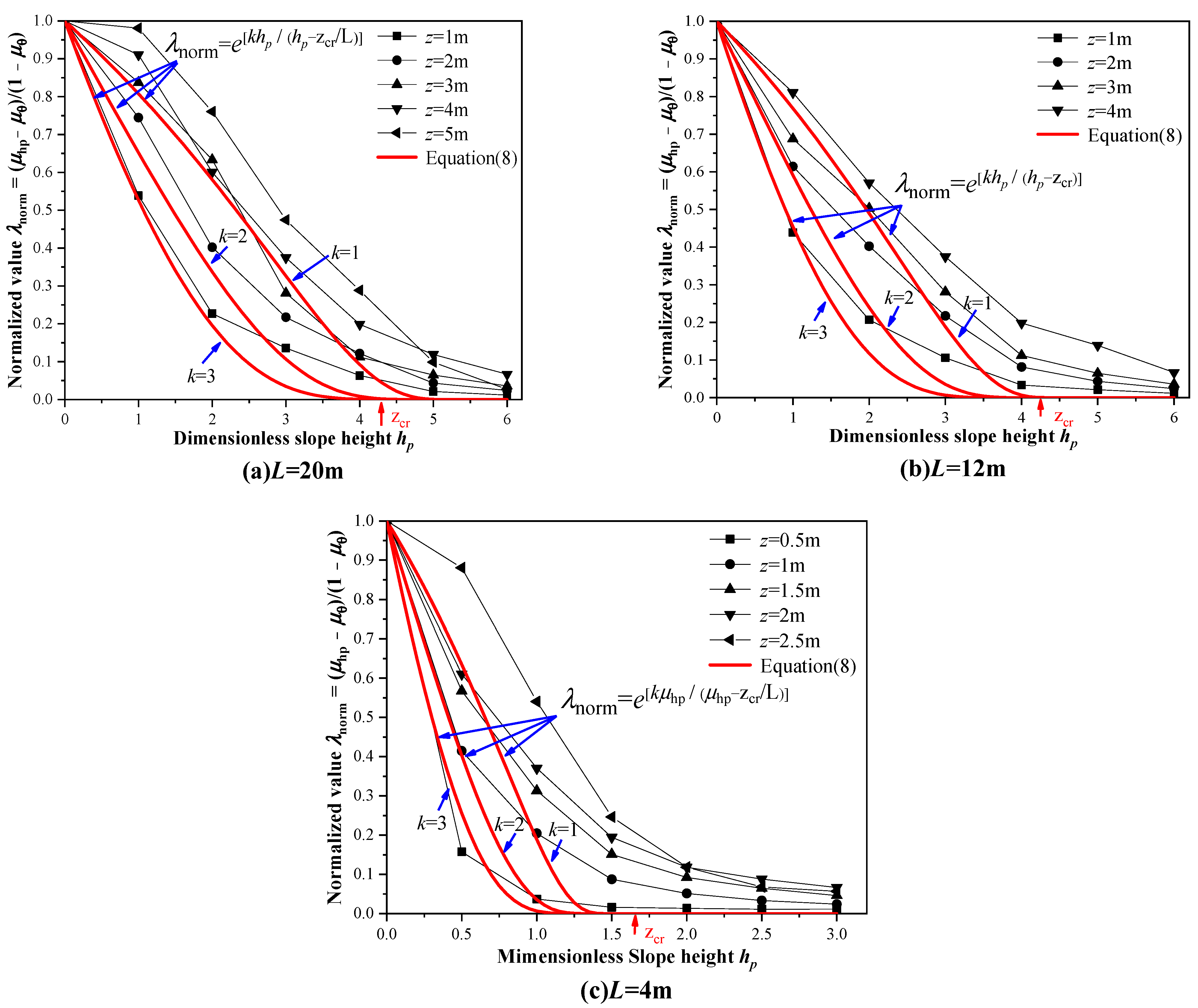
As shown in Figure 11, the shape of the passive wedge is a triangle and does not change when h p z cr / L . At this time, the reduction factor ( μ h p ) remains the same as μ θ . Furthermore, the soil–pile system is not affected by the slope for cases with level ground ( h p = 0 ) and μ h p = 1 . Thus, a conclusion can be drawn that μ h p decreases from 1 to μ θ as h p increases from 0 to z cr . To figure out the problem of how μ h p varies, a normalized reduction factor λ norm is proposed in this paper that can be calculated as follows:
λ norm = ( μ h p μ θ ) / 1 μ θ
Equation (14) uses the normalized method to reflect the weight of μ h p for different values of μ θ . Figure 16 shows the nonlinear variation of λ norm with h p for different depths of piles. At deep depths, though curves show differences to shallow-depth curves, these curves are not considered because the μ h p of these curves is close to 1. Thus, the relationship between λ norm and h p is provided in a nonlinear form as follows:
λ norm = μ h p μ θ 1 μ θ = e [ k h p h p z cr / L ]
Rearranging Equation (15), μ h p can be calculated as the following when h p < z cr / L :
μ h p = f h p , μ θ = μ θ + 1 μ θ e k h p h p z cr / L ( h p < z cr / L )
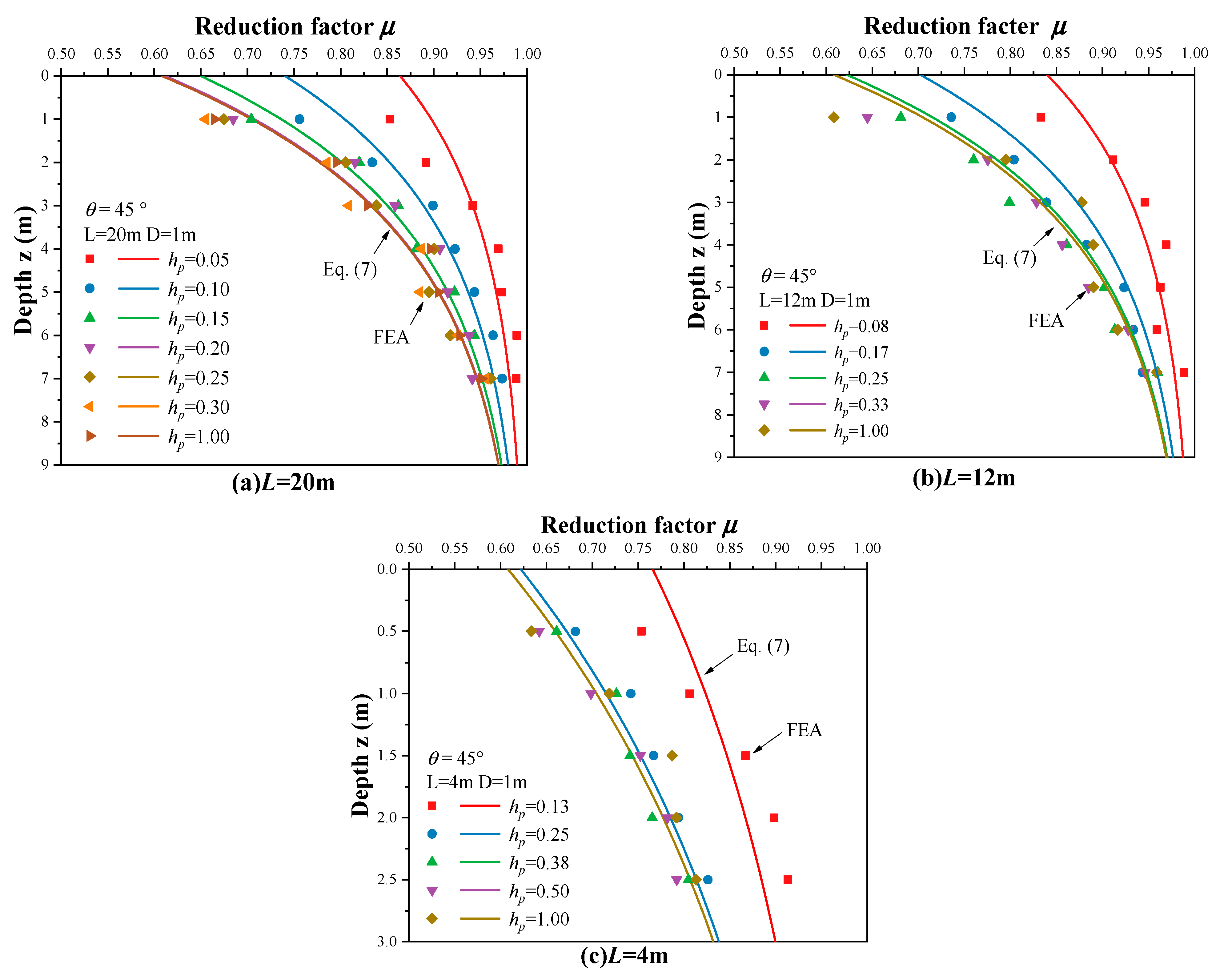
where z cr is calculated to be 1.6 m, 4.2 m, and 4.26 m with Equations (11) and (13), for pile lengths of 4 m, 12 m, and 20 m, respectively; k is a parameter that controls the shape of the curve, as shown in Figure 16. Equation (16) reflects more characteristics of shallow depths with the increase of k . To fit more cases of depths, k = 2 is considered to be suitable and reasonable. Additionally, the numbers “1” and “ μ θ ” in Equation (16) can be regarded as the reduction factor of the slope bottom (level ground) and that of the slope, respectively.
Finally, Equation (10) can be expressed as:
μ h p = μ θ + 1 μ θ e ( 2 h p h p z cr / L ) , h p < z cr / L μ θ , h p z cr / L
Figure 17 shows the curves derived using Equation (17) and the data from FEA, which show good agreement between the prediction and the simulation results.

4.2.2. Case 5: Variation of Pile Location on Slope ( l p )

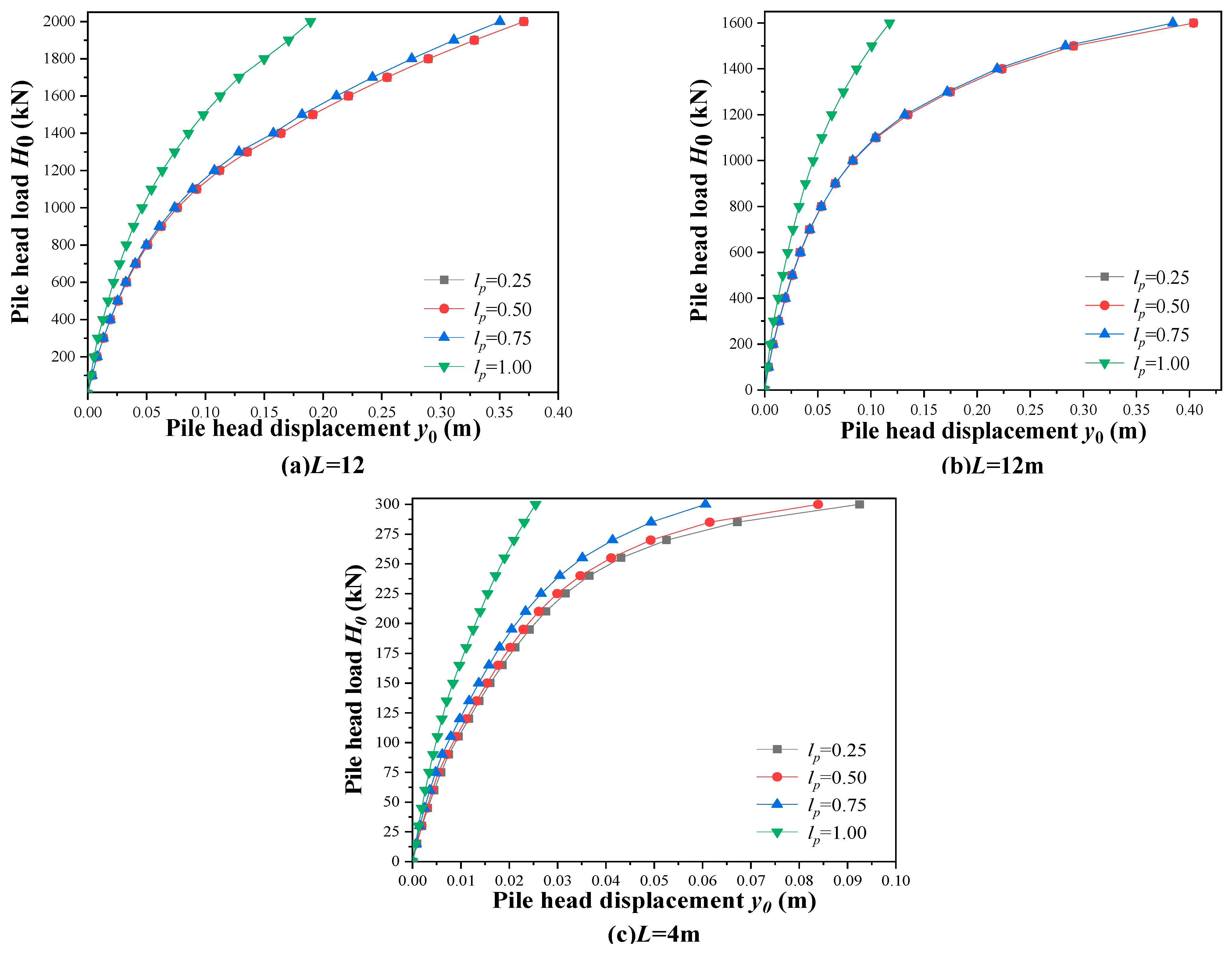
In this case, the pile is installed on the slope, at a distance ( l p ) away from the crest, as shown in Table 1(e), where l p = h / L . Figure 18 shows that the lateral bearing capacity increases with l p , increasing from zero to one for cases where the slope angle θ = 45 ° . It is obvious that, although l p increases in a linear way, the lateral bearing capacity increases nonlinearly. Considering that the soil–pile response is independent of the soil behind the pile, as Case 3 shows, the case of variation of pile location on slope ( l p ) (case 5) can be regarded as the combination of Case 3 and Case 4. Replacing h p in Equation (17) with H / L l p , the reduction factor ( μ l p ) can be calculated using the following equation:
μ l p = μ θ + 1 μ θ e [ k H / L l p H / L l p z cr / L ] , l p > H z cr / L μ θ , l p H z cr / L

5. Comparison and Validation

5.1. Comparison with Other Methods

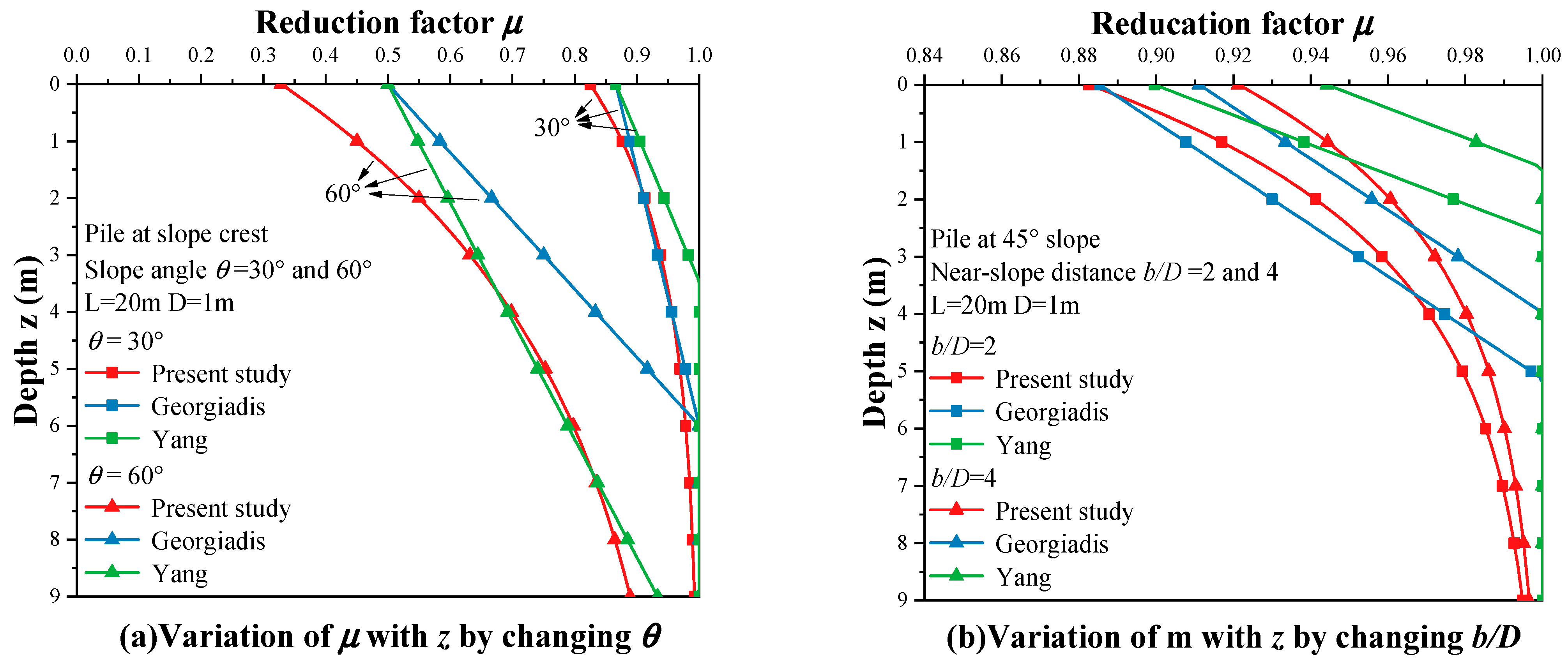
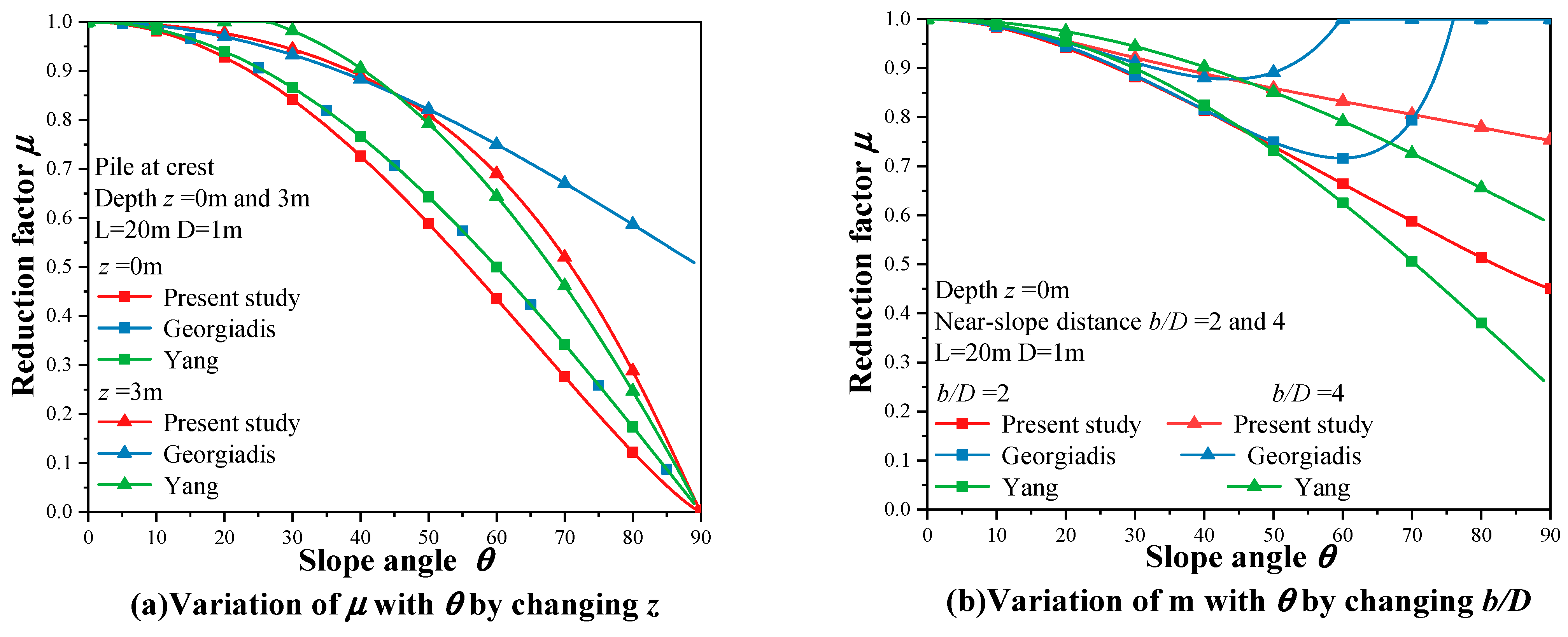
Since Georgiadis and Georgiadis [18] proposed the concept of the reduction factor ( μ ) of the initial stiffness for soil–pile response in undrained clay slopes, some researchers have developed the method. Figure 19 and Figure 20 show the comparison of μ fromthe present study with the methods of Georgiadis and Georgiadis [18,22] and Yang et al. [16]. Figure 19a shows that μ approaches one with depth for both the present study and the method of Yang et al., but equals one below z = 6 D for the method of Georgiadis and Georgiadis. Moreover, the present study shows a relatively smaller value of μ , which is more conservative for the engineering design. Figure 19b shows that the value of μ in the present study is similar to the μ value of the method of Georgiadis and Georgiadis, and the μ value of the method of Yang et al. is larger.
Figure 20a shows that all the μ values of the three methods are nearly the same for small angle slopes. As the slope angle increases, the trend of μ in the present study is similar to Yang et al.’s method. However, Georgiadis and Georgiadis’ method only shows good agreement with real cases for small slope angles, which is also indicated in Georgiadis and Georgiadis’ study [18]. Figure 20b shows the similar trend of μ for both the present study and Yang et al.’s method, and the μ value of Yang et al.’s method is smaller for large slope angles. In the same way, the μ value of Georgiadis and Georgiadis’ method only shows good agreement for small slope angles, and the μ value of the present study is better predicted for large slope angles. Additionally, note that both Georgiadis and Georgiadis’ method and Yang et al.’s method cannot predict the ideal case of the slope angle θ = 90 ° , but it can be obtained by using the method of the present study.

5.2. Application to Test Cases

The present study is validated by two pile tests in this section. Usually, the soil–pile response is reflected by monitoring the pile head load ( H 0 ) and displacement ( y 0 ), which is known to be a H 0 y 0 curve. The hyperbolic p-y curves in Equation (1) and the deflection differential equation are used to derive H 0 y 0 curves as follows:
E p I p d 4 y d z 4 + p = 0
The finite difference method is used to transform differential equations into difference equations. The displacement of the laterally loaded pile can be obtained by solving these difference equations. Then the pile head load–displacement curve ( H 0 y 0 ) can also be obtained.
The values of the parameters used to calculate H 0 y 0 curves are as shown in Table 5, where e is the height of the load applied above the ground level; c u is undrained shear strength; and E s is Young’s modulus of the soil.

5.2.1. Case 1: Bhushan’s Pile Test

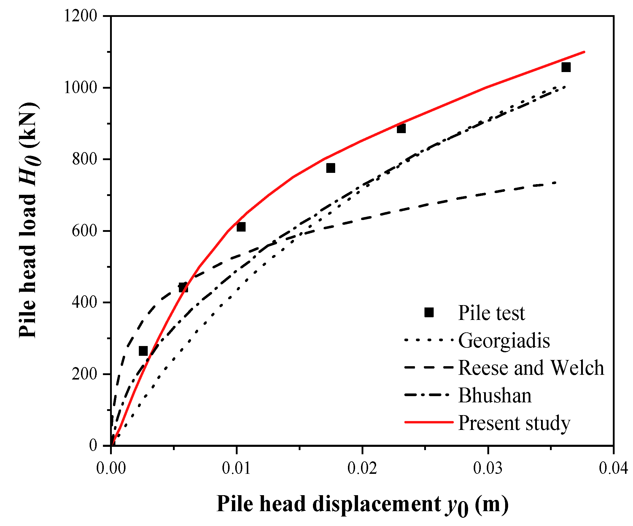
A laterally loaded rigid pile test at a stiff clay slope crest by Bhushan et al. [42] was used to validate the present study, together with the theoretical results of Reese and Welch [40], Bhushan et al. [42], and Georgiadis and Georgiadis [18]. The case is the same as the case in Section 4.1.1 where θ = 20 ° , and the parameter values are shown in Table 5. The calculation method of p u and K i is the same as the method of Georgiadis and Georgiadis [18], as seen in Appendix A, and the method of the present study is used to calculate μ θ = K i θ / K i . The H 0 y 0 curves are shown in Figure 21, which shows better agreement with the pile test when using the method of μ in the present study.

5.2.2. Case 2: Yang’s Pile Test

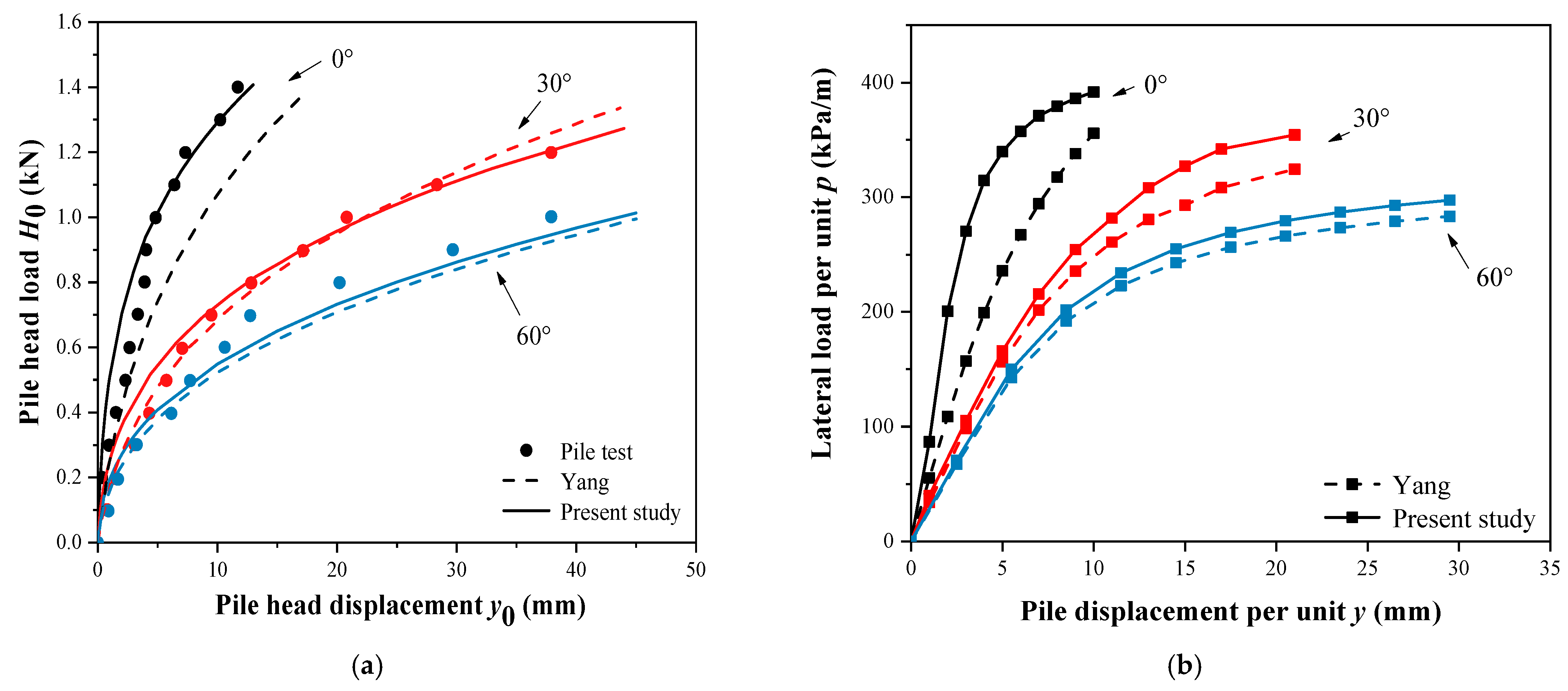
A lateral flexible pile test in the middle of the clay slope by Yang et al. [16] was used to validate the present study. The case is the same as the case in Section 4.2.1 where h p / L = 0.5 , and the parameter values are shown in Table 5. The calculation method of p u and K i is the same as the method of Yang et al. [16], as seen in Appendix A, and the method of the present study is used to calculate μ h p = K ih p / K i . Note that z t is calculated to be 0.19 m in the case of the pile test. The H 0 y 0 curves and p-y curves at z = 0   m depth are shown in Figure 22. Compared with Yang et al.’s method, the result of the present study proves to have good agreement with the pile test for the large load when the slope angle is small. Moreover, when the slope angle is large, the results of the present study are similar to the result of Yang et al.’s method. Additionally, the lateral load per unit (p) is calculated to be larger than the results of Yang et al.

6. Conclusions

The paper proposes nonlinear prediction methods for the slope effect ( μ ) on the initial stiffness ( K i ) of p-y curves of the undrained laterally loaded pile. Five cases are classified to analyze the slope effect ( μ ) on the initial stiffness ( K i ) of a laterally loaded pile, based on the pile–slope position relationship. A series of FEA simulations were conducted, and the data were derived to calculate μ . Nonlinear models of μ were established for these five cases, and parameters in the models were calibrated using the results of FEA. The nonlinear models showed good agreement with FEA results. Compared with other researchers’ μ models, the method in this paper is in a reasonable range and can predict more cases. The test cases were used to validate the proposed model, which shows that the p-y curves are in better agreement with test results when using the model of the present study. Additionally, some other conclusions were also obtained:
(1)
The pile–soil response in undrained clay conditions was nearly independent of the dimensionless pile head-crest distance ( h / L ) for the “no slope geometry effect” case, which can be explained by the theory of Coulomb earth pressure.
(2)
The depth of the first turning point of the pile under undrained loading was explored as 0.8 L for the flexible pile, 0.7 L for the elastic pile, and 0.6 L flex for the flexible pile. The soil–pile response for the case of h p z cr / L was found to be the same as the case of h p 1 (“no slope geometry effect” case).
(3)
Compared with the available initial stiffness ( μ ) calculation methods, the results are more reasonable for large slope angle cases, and can predict some ideal cases, such as the case of θ = 90 ° , by using the method of the present study.

Author Contributions

Conceptualization, L.P. and C.J.; Funding acquisition, C.J.; Methodology, L.P.; Resources, C.J.; Software, L.C.; Supervision, L.C.; Validation, L.C.; Visualization, L.C.; Writing—original draft, L.P.; Writing—review and editing, C.J. All authors have read and agreed to the published version of the manuscript.

Funding

This research was funded by the National Natural Science Foundation of China, grant number 51978665.

Institutional Review Board Statement

Not applicable.

Informed Consent Statement

Not applicable.

Data Availability Statement

The data presented in this study are available on request from the corresponding author.

Conflicts of Interest

The authors declare no conflict of interest.

Appendix A. Theoretical Method of Georgiadis and Georgiadis [18] and Yang et al. [16]

For undrained laterally loaded piles, the ultimate lateral load per unit pile length ( p u ) in Equation (1) is calculated by:
p u = N p c u D
where N p was calculated by Georgiadis and Georgiadis [18] for piles at the slope crest:
N p = N pu N pu N p 0 cos θ e λ z / D / 1 + tan θ
and calculated by Yang et al. [16] for piles in the middle of the slope, as following:
N p = N pu N pu N p 0 α 1 2 α 2 2 e λ z / D α 1 2
where α 1 = 1 / 1 + tan θ , α 2 = 1 sin θ 1 + sin θ / 2 ; and N pu , N p 0 , and λ can be calculated as follows:
N pu = π + 2 Δ + 2 cos Δ + 4 ( cos Δ 2 + sin Δ 2 )
N p 0 = 2 + 1.5 α
λ = 0.55 0.15 α
where Δ = 1 / sin α and α is the adhesion factor, which is related to c u and can be determined by figuring out α versus c u relationships from Georgiadis and Georgiadis’ [18] study.
The initial stiffness K i in Equation (1) is calculated by:
K i = 3 E s ( E s D 4 E p I p ) 1 / 12
The linear reduction factor proposed by Georgiadis and Georgiadis [18] is given as:
μ = K i θ K i 0 = cos θ + 1 cos θ 6 D [ z D + ( b D 0.5 ) tan θ ] 1
It is given by Yang et al. [31] as:
μ = K i θ K i 0 = cos θ + z 6 D tan θ 1 cos θ

Appendix B. The Process of Deriving the K i θ from Simulation Results

Figure A1. Process of deriving K i θ from simulation results.
Jmse 10 01684 g0a1

References

  1. Wang, S.; Wang, P.; Zhai, H.; Zhang, Q.; Chen, L.; Duan, L.; Liu, Y.; Jeng, D. Experimental study for wave-induced pore-water pressures in a porous seabed around a mono-pile. J. Mar. Sci. Eng. 2019, 7, 237–255. [Google Scholar]
  2. Wan, Z.; Dai, G.; Gong, W. Field study on post-grouting effects of cast-in-place bored piles in extra-thick fine sand layers. Acta Geotech. 2019, 14, 1357–1377. [Google Scholar]
  3. Liu, X.; Lu, Y.; Yu, H.; Ma, L.; Ma, L.; Li, X.; Li, W.; Zhang, H.; Bian, C. In-situ observation of storm-induced wave-supported fluid mud occurrence in the subaqueous Yellow River delta. J. Geophys. Res. Ocean. 2022, 127, e2021JC018190. [Google Scholar] [CrossRef]
  4. Liu, X.; Yang, Q.; Wang, Y.; Jeng, D.; Sturm, H. New advances in marine engineering geology. J. Mar. Sci. Eng. 2021, 9, 66. [Google Scholar]
  5. Rajashree, S.; Sitharam, T. Nonlinear finite-element modeling of batter piles under lateral load. J. Geotech. Geoenviron. Eng. 2001, 127, 604–612. [Google Scholar]
  6. Kim, B.; Kim, N.; Jin, L.; Kim, Y. Experimental load–transfer curves of laterally loaded piles in Nak-Dong river sand. J. Geotech. Geoenviron. Eng. 2004, 130, 416–425. [Google Scholar]
  7. Sawant, V.; Shukla, S. Effect of edge distance from the slope crest on the response of a laterally loaded pile in sloping ground. Geotech. Geol. Eng. 2014, 32, 197–204. [Google Scholar] [CrossRef]
  8. Yin, P.; He, W.; Yang, Z. A Simplified Nonlinear Method for a Laterally Loaded Pile in Sloping Ground. Adv. Civ. Eng. 2018, 2018, 5438618. [Google Scholar] [CrossRef] [Green Version]
  9. Jiang, C.; Zhang, Z.; He, J. Nonlinear analysis of combined loaded rigid piles in cohesionless soil slope. Comput. Geotech. 2020, 117, 117. [Google Scholar] [CrossRef]
  10. Matlock, H. Correlation for design of laterally loaded piles in soft clay. In Proceedings of the 2nd Offshore Technology Conference, Houston, TX, USA, 22–24 April 1970; pp. 577–594. [Google Scholar]
  11. O’Neill, M.W.; Gazioglu, S.M. An Evaluation of P-y Relationships in Clays; University of Houston, Department of Civil Engineering: Houston, TX, USA, 1984. [Google Scholar]
  12. Sharafi, H.; Maleki, Y.; Karimpour-Fard, M. Three-dimensional finite difference modeling of static soil-pile interactions to calculate p-y curves in pile-supported slopes. Arab. J. Geosci. 2015, 9, 5. [Google Scholar] [CrossRef]
  13. Yin, J.; Li, S.; Sun, L.; Li, T. Pile installation assessment of offshore wind jacket foundation in completely weathered rock: A case study of the South China Sea. J. Mar. Sci. Eng. 2022, 10, 900. [Google Scholar] [CrossRef]
  14. Sun, W. A p-y model for predicting the lateral nonlinear interaction between pile and soil-rock mixture material based on discrete element modeling. Simul. Model. Pract. Theory 2020, 100, 102060. [Google Scholar] [CrossRef]
  15. Rathod, D.; Muthukkumaran, K.; Thallak, S. Experimental investigation on behavior of a laterally loaded single pile located on sloping ground. Int. J. Geomech. 2019, 19, 04019021. [Google Scholar] [CrossRef]
  16. Yang, M.; Deng, B.; Zhao, M. Experimental and theoretical studies of laterally loaded single piles in slopes. J. Zhejiang Univ. Sci. A 2019, 20, 838–851. [Google Scholar] [CrossRef]
  17. Nimityongskul, N.; Kawamata, Y.; Rayamajhi, D.; Scott, A. Full-scale tests on effects of slope on lateral capacity of piles installed in cohesive soils. J. Geotech. Geoenviron. Eng. 2018, 144, 04017103. [Google Scholar] [CrossRef]
  18. Georgiadis, K.; Georgiadis, M. Development of p-y curves for undrained response of piles near slopes. Comput. Geotech. 2012, 40, 53–61. [Google Scholar] [CrossRef]
  19. Peng, W.; Zhao, M.; Yao, X.; Yang, C.; Zhao, H. Analysis of laterally loaded piles in sloping ground using a modified strain wedge model. Comput. Geotech. 2018, 107, 163–175. [Google Scholar] [CrossRef]
  20. Liu, J.; Guo, Z.; Han, B. Load transfer of offshore open-ended piles considering the effect of soil plugging. J. Mar. Sci. Eng. 2019, 7, 313. [Google Scholar] [CrossRef] [Green Version]
  21. Reese, L.; Cox, W.; Koop, F. Analysis of laterally loaded piles in sand. In Offshore Technology in Civil Engineering: Hall of Fame Papers from the Early Years; American Society of Civil Engineers: Reston, VA, USA, 1974; pp. 95–105. [Google Scholar]
  22. Georgiadis, K.; Georgiadis, M. Undrained lateral pile response in sloping ground. J. Geotech. Geoenviron. Eng. 2010, 136, 1489–1500. [Google Scholar] [CrossRef]
  23. Brown, D.; Shie, C. Some numerical experiments with a three dimensional finite element model of a laterally loaded pile. Comput. Geotech. 1991, 12, 149–162. [Google Scholar] [CrossRef]
  24. Murff, J.; Hamilton, J. P-ultimate for undrained analysis of laterally loaded piles. J. Geotech. Eng. 1993, 119, 91–107. [Google Scholar] [CrossRef]
  25. Pedram, B. Effects of pile shape in improving the performance of monopiles embedded in onshore clays. Can. Geotech. J. 2015, 52, 1144–1158. [Google Scholar] [CrossRef]
  26. Vesic, A. Bending of beams resting on isotropic elastic solid. J. Eng. Mech. Div. 1961, 87, 35–54. [Google Scholar] [CrossRef]
  27. Carter, D.P. A Non-Linear Soil Model for Predicting Lateral Pile Response. Ph.D. Thesis, Department of Civil and Environmental Engineering, University of Auckland, Auckland, New Zealand, 1984. [Google Scholar]
  28. Kim, Y.; Jeong, S.; Lee, S. Wedge failure analysis of soil resistance on laterally loaded piles in clay. J. Geotech. Geoenviron. Eng. 2011, 137, 678–694. [Google Scholar] [CrossRef]
  29. Jeong, S.; Kim, Y.; Kim, J. Influence on lateral rigidity of offshore piles using proposed p–y curves. Ocean Eng. 2011, 38, 397–408. [Google Scholar] [CrossRef]
  30. Yang, Y.; Shen, M.; Juang, C. Assessing initial stiffness models for laterally loaded piles in undrained clay: Robust design perspective. J. Geotech. Geoenviron. Eng. 2019, 145, 04019073. [Google Scholar]
  31. Yang, M.; Zhu, L.; Luo, H.; Feng, C. Experiment and numerical simulation of p-y curve method for laterally loaded single pile in sloping ground. Jounral Highw. Transp. Res. Dev. 2017, 24, 83–90. [Google Scholar]
  32. Terzaghi, K. Evaluation of coefficient of subgrade reaction. Geotechnique 1955, 5, 297–326. [Google Scholar] [CrossRef]
  33. Poulos, H. Single pile response to cyclic lateral load. J. Geotech. Geoenviron. Eng. 1982, 108, 355–375. [Google Scholar] [CrossRef]
  34. Zhou, J.; Gong, X.; Wang, K.; Zhang, R.; Yan, J. A simplified nonlinear calculation method to describe the settlement of pre-bored grouting planted nodular piles. J. Zhejiang Univ. Sci. A 2007, 18, 895–909. [Google Scholar] [CrossRef]
  35. Wang, A.; Zhang, D.; Deng, Y. Lateral response of single piles in cement-improved soil: Numerical and theoretical investigation. Comput. Geotech. 2018, 102, 164–178. [Google Scholar] [CrossRef]
  36. Sun, Y.; Xu, C.; Du, X.; Naggar, M.; Jia, J. Nonlinear lateral response of offshore large-diameter monopile in sand. Ocean. Eng. 2020, 216, 108013. [Google Scholar] [CrossRef]
  37. Yang, X.; Zhang, C.; Huang, M.; Yuan, H. Lateral loading of a pile using strain wedge model and its application under scouring. Mar. Georesour. Geotechnol. 2018, 36, 340–350. [Google Scholar] [CrossRef]
  38. Chen, L.; Jiang, C.; Pang, L.; Liu, P. Lateral soil resistance of rigid pile in cohesionless soil on slope. Comput. Geotech. 2021, 135, 104163. [Google Scholar] [CrossRef]
  39. Sivapriya, S.; Gandhi, S. Soil–Structure Interaction of Pile in a Sloping Ground Under Different Loading Conditions. Geotech. Geol. Eng. 2019, 38, 1185–1194. [Google Scholar] [CrossRef]
  40. Reese, L.; Wlech, R. Lateral loading of deep foundations in stiff clay. J. Geotech. Eng. Div. 1975, 101, 633–649. [Google Scholar] [CrossRef]
  41. Reese, L.; Isenhower, W.; Wang, S. Analysis of Design of Shallow and Deep Foundations; John Wiley and Sons: Hoboken, NJ, USA, 2006. [Google Scholar]
  42. Bhushan, K.; Haley, S.; Fong, P. Lateral load tests on drilled piers in stiff clays. J. Geotech. Eng. Div. 1979, 105, 969–985. [Google Scholar] [CrossRef]
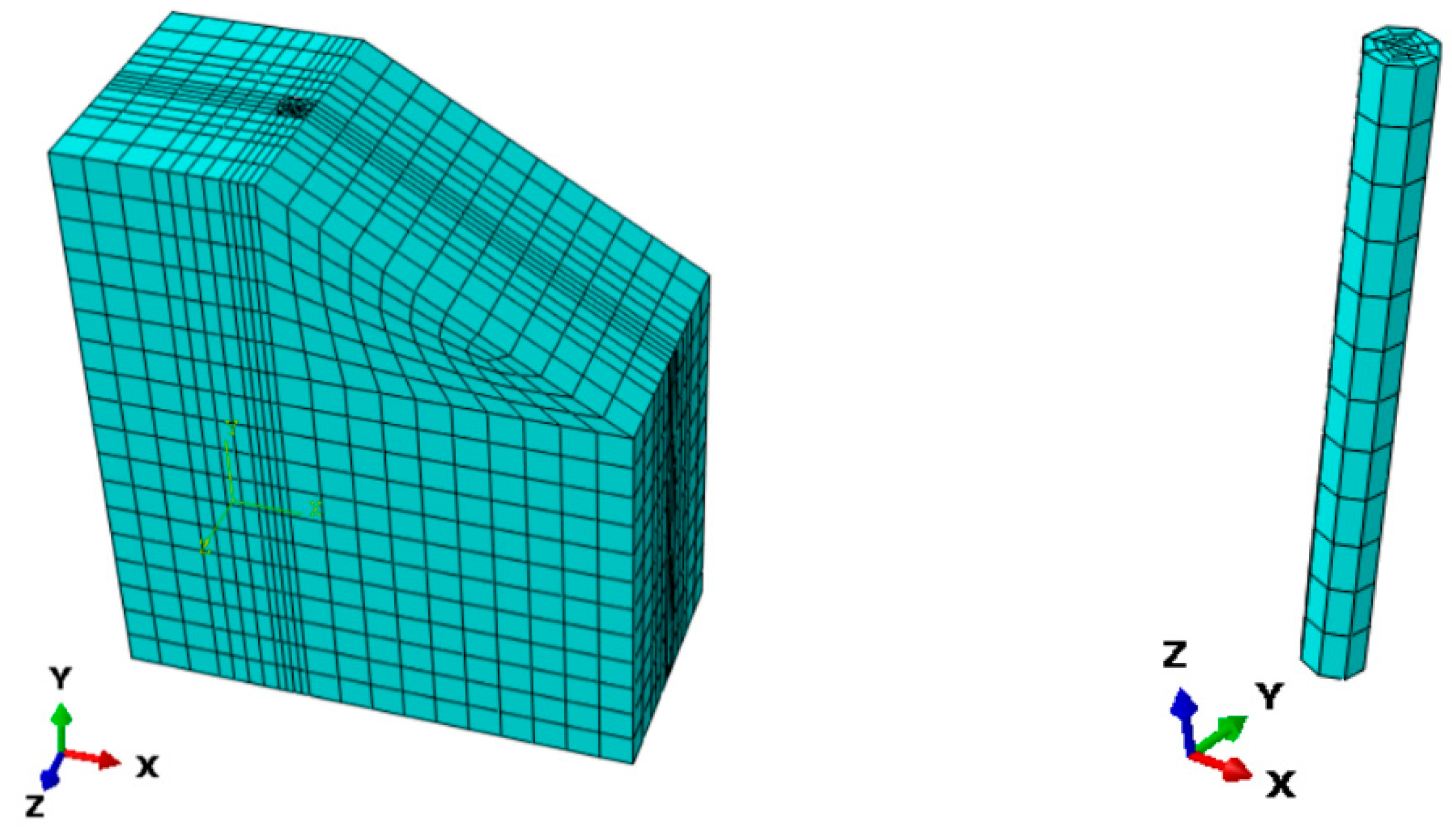
Figure 1. Typical 3D finite-element meshing in ABAQUS.
Jmse 10 01684 g001
Figure 2. Comparison of FEA results with the theoretical method of the 20 m length pile and 15°, 45°, and 60° slope angles.
Jmse 10 01684 g002
Figure 3. Effect of θ on μ θ by FEA for (a) L = 20 m; (b) L = 12 m; (c) L = 4 m.
Jmse 10 01684 g003
Figure 4. Transition from a pile at the slope crest to a pile near the slope crest.
Jmse 10 01684 g004
Figure 5. Effect of b / D on μ b / D by deriving the results of FEA for θ = 90 ° .
Jmse 10 01684 g005
Figure 6. Distribution of non-dimensional parameter α .
Jmse 10 01684 g006
Figure 7. Effect of b / D on μ for (a) θ = 30 ° ; (b)   θ = 60 ° .
Jmse 10 01684 g007
Figure 8. Effect of the slope height on pile head displacement of piles.
Jmse 10 01684 g008
Figure 9. Effect of the dimensionless slope height ( h p ) on pile-head displacement for slope angle θ = 45 ° . Piles of (a) 20 m, (b) 12 m, and (c) 4 m lengths.
Jmse 10 01684 g009
Figure 10. The wedge failure model at shallow depth for level ground. (a) H 0 and (b) H 1 .
Jmse 10 01684 g010
Figure 11. The theoretical largest passive wedge for (a) h p 1 and (b) h p 2 .
Jmse 10 01684 g011
Figure 12. (a) Different passive wedges with slope angle ( θ ) and (b) variation of z cr with slope angle ( θ ).
Jmse 10 01684 g012
Figure 13. The value of z t / L derived by FEA. (a) 4 m length pile, (b) 12 m length pile, and (c) 20 m length pile.
Jmse 10 01684 g013
Figure 14. The variation of the z t / L with h p derived by FEA.
Jmse 10 01684 g014
Figure 15. The depth ( z t ) of the first turning point of pile for (a) a rigid pile, (b) a elastic pile and (c) a flexible pile.
Jmse 10 01684 g015
Figure 16. The variation of λ n o r m with h p for (a) L = 20   m ,   (b) L = 12   m , and (c)   L = 4   m .
Jmse 10 01684 g016
Figure 17. Effect of h p on μ for pile length of (a) 20   m , (b) 12   m , and (c)   4   m .
Jmse 10 01684 g017
Figure 18. Effect of pile location on slope ( l p ) on pile head displacement from the data of FEA, for slope angle θ = 45 ° . Piles of (a) 20 m, (b) 12 m, and (c) 4 m lengths.
Jmse 10 01684 g018
Figure 19. Comparison of the variation of μ with z by changing (a) θ and (b) b / D [16,18].
Jmse 10 01684 g019
Figure 20. Comparison of the variation of μ with θ by changing (a) z and (b) b / D [16,18].
Jmse 10 01684 g020
Figure 21. Validation with rigid pile test at the stiffness clay slope crest [18,40,42].
Jmse 10 01684 g021
Figure 22. Validation with the flexible pile test in the middle of the clay slope.(a) H 0 y 0 curves and (b) p y curves at depth of z = 0   m [16].
Jmse 10 01684 g022
Table 1. Pile-slope geometry relationships.
Pile-Slope Geometry RelationshipsVariables
(a) Slope Angle θ (b) Dimensionless Near-Slope Distance b / D (c) Dimensionless Pile Head-Crest Distance h / L
No slope geometry effectJmse 10 01684 i001Jmse 10 01684 i002Jmse 10 01684 i003
Pile-Slope Geometry RelationshipsVariables
(d) Dimensionless Slope Height h p (e) Pile Location in the Slope l p
Existence of the slope geometry effectJmse 10 01684 i004Jmse 10 01684 i005
Table 2. The description of some used symbols.
SymbolsDescription
K i Initial stiffness
K i 0 Initial stiffness in the level ground condition
K i θ Initial stiffness in the slope condition
K ii Initial stiffness at the ground surface
μ Reduction factor
μ θ Reduction factor in the “no slope geometry effect” case with varying ( θ )
μ b / D Reduction factor in the “no slope geometry effect” case with varying ( b / D )
μ h / D Reduction factor in the “no slope geometry effect” case with varying ( h / D )
μ h p Reduction factor in the “existence of the slope geometry effect” case with varying ( h p )
μ l p Reduction factor in the “existence of the slope geometry effect” case with varying ( l p )
Table 3. Soil and pile properties.
PropertiesValue
Soil
Young’s module E s (MPa)14
Undrained shear strength c u (kPa)70
Bulk unit weight γ s (kN/m3)18
Poisson’s ratio ν s 0.49
Adhesion factor α s 0.5
Pile
Young’s module E p (MPa)2.9 × 10⁴
Bulk unit weight γ p (kN/m3)25
Poisson’s ratio ν p 0.1
Pile length L (m)4, 12, 20
Pile diameter D (m)1
Table 4. Variables values.
VariablesConditionsValues
“no slope geometry effect” case
Slope angle θ L = 4 ,   12 ,   20   m ; pile at crest0, 15, 30, 45, 60, 75, 90
Dimensionless near-slope distance b / D L = 20   m ;   θ = 30 ° ,   60 ° ,   90 ° 1, 2, 3, 4, 5, 6
Dimensionless pile head-crest distance h / L L = 4 ,   12 ,   20   m ;   θ = 45 ° ; pile in slope0.5, 1, 1.5, 2
“existence of the slope geometry effect” case
Dimensionless slope height h p = h / L L = 4 ,   12 ,   20   m ;   θ = 45 ° ; pile in slope h p = 0.5, 1, 1.5, 2
Pile location in slope l p = h / L L = 4 ,   12 ,   20   m ;   θ = 45 ° ; pile in slope l p = 0.25, 0.5, 0.75, 1
Table 5. Summary of pile load tests.
Pile TestGeometrical CharacteristicsSoil Properties
L (m) D (m) E p I p   ( kN   m 2 ) e (m) θ c u   ( kPa ) E s   ( kPa )
Bhushan5.1851.222.25 × 1060.232022024,440
Yang10.0250.10.150, 30, 6053.230,120
Publisher’s Note: MDPI stays neutral with regard to jurisdictional claims in published maps and institutional affiliations.