Significant Wave Height Prediction in the South China Sea Based on the ConvLSTM Algorithm

Abstract

Deep learning methods have excellent prospects for application in wave forecasting research. This study employed the convolutional LSTM (ConvLSTM) algorithm to predict the South China Sea (SCS) significant wave height (SWH). Three prediction models were established to investigate the influences of setting different parameters and using multiple training data on the forecasting effects. Compared with the SWH data from the China–France Ocean Satellite (CFOSAT), the SWH of WAVEWATCH III (WWIII) from the pacific islands ocean observing system are accurate enough to be used as training data for the ConvLSTM-based SWH prediction model. Model A was preliminarily established by only using the SWH from WWIII as the training data, and 20 sensitivity experiments were carried out to investigate the influences of different parameter settings on the forecasting effect of Model A. The experimental results showed that Model A has the best forecasting effect when using three years of training data and three hourly input data. With the same parameter settings as the best prediction performance Model A, Model B and C were also established by using more different training data. Model B used the wind shear velocity and SWH as training and input data. When making a 24-h SWH forecast, compared with Model A, the root mean square error (RMSE) of Model B is decreased by 17.6%, the correlation coefficient (CC) is increased by 2.90%, and the mean absolute percentage error (MAPE) is reduced by 12.2%. Model C used the SWH, wind shear velocity, wind and wave direction as training and input data. When making a 24-h SWH forecast, compared with Model A, the RMSE of Model C decreased by 19.0%, the CC increased by 2.65%, and the MAPE decreased by 14.8%. As the performance of the ConvLSTM-based prediction model mainly rely on the SWH training data. All the ConvLSTM-based prediction models show a greater RMSE in the nearshore area than that in the deep area of SCS and also show a greater RMSE during the period of typhoon transit than that without typhoon. Considering the wind shear velocity, wind, and wave direction also used as training data will improve the performance of SWH prediction.

1. Introduction

The South China Sea (SCS) is a large semi-enclosed marginal sea and the third-largest continental marginal sea in the world (after the Coral Sea and the Arabian Sea) [1]. With abundant mineral, oil and gas, and fishery resources, the SCS has a considerable variation in water depth [2], including deep-sea and shallow nearshore areas. The climate of the SCS is dominated by the southwest monsoon in summer and the northeast monsoon in winter due to the East Asian monsoon system [3]. The topographic characteristics of the SCS and the monsoon system significantly influence the wave characteristics of the SCS. Accurate wave forecasting can effectively improve the safety of marine activities in the SCS, such as fishing, exploration, power generation, and shipping, and the efficiency of marine operation, as well as reduce marine accidents [4,5,6].

Significant wave height (SWH) is one of the most critical elements of wave forecasting. There are two main categories of traditional wave forecasting methods. The first ones are the emerged semi-analytical and semi-empirical methods, such as the Sverdroup–Munk–Bretscheider (SMB) method [7] and the Pierson–Neumann–James (PNJ) method [8]. Although these empirical methods are fast and accurate, they are not theoretically rigorous enough to describe the conditions of wave influence in detail. They are only applicable to a limited case [9]. The second type of method of wave forecasting is based on numerical wave models, which are the most widely used methods of wave forecasting now. The principle of numerical wave models is to obtain wave height, period, and other information by solving the wave spectrum equations for physical processes in the ocean. The most mature models are the third-generation wave models, such as wave model (WAM) [10], simulating waves nearshore (SWAN) [11,12], and WAVEWATCH III (WWIII) [13,14]. However, their theoretical and computational complexity consumes many computational resources and time [15,16].

In recent years, with the development of soft-computing methods (SCM), artificial neural networks, fuzzy computing, machine learning, and other SCM have been widely used in wave forecasting. For example, three studies [9,17,18] applied artificial neural network (ANN) models in wave height prediction. Compared with autoregressive models, ANN methods have the advantages of flexibility and adaptability [19]. However, ANN is not extensively business oriented because of its limited predictive capability [20]. In order to overcome these problems, extreme learning machines (ELM) [21,22,23,24], support vector machines (SVM) [25,26], adaptive network-based fuzzy inference systems (ANFIS) [27], Bayesian networks (BN) [28,29], and rough set theory (RST) [30] methods were also applied to the forecasting of SWH.

The recurrent neural network (RNN) and its variant method, the long short-term memory (LSTM) network [31], have unique advantages in solving prediction problems. Gao et al. [20] developed a wave height prediction model based on the LSTM neural network for the Bohai Sea gauging stations. They demonstrated that the LSTM model gave significantly better results than feedforward neural networks (FNN) and support vector regression (SVR) models. Many combined LSTM and other methods were applied in recent studies in SWH. For example, Ni and Ma [32] combined principal component analysis (PCA) with LSTM to predict wave height and compared the results with linear regression (LR), regression tree (TR), SVM, and Gaussian process regression (GPR), and the results performed much better in terms of performance metrics and time consumption. Fan et al. [19] combined SWAN with LSTM and found that the SWAN-LSTM model outperformed ELM and SVM in prediction. Pirhooshyaran and Snyder [33] combined LSTM neural networks with Bayesian hyperparametric optimization and elastic network methods. Sequence-to-sequence neural networks were developed for the first time, and the prediction results of SWH were superior in validation.

The previous LSTM network model for SWH prediction was limited to the single-point prediction of spatial elements. To address the problem of prediction of spatio-temporal sequences in the proximity forecasting of precipitation, Shi et al. [34] developed a convolutional LSTM (ConvLSTM) algorithm. The ConvLSTM algorithm is a predictive model of variables constructed by establishing relationships between input and predictor variables with a sufficient amount of training data. Experiments have shown that the ConvLSTM network can better capture the spatio-temporal correlation of elements and consistently outperforms other algorithms, such as fully connected LSTM (FC-LSTM). Previous studies have demonstrated the feasibility of employing the ConvLSTM algorithm for SWH prediction. For example, Choi et al. [35] predicted SWH from continuous ocean images based on a two-way ConvLSTM regression model, and the model predictions yielded meager error rates in terms of mean absolute error (MAE) and mean absolute percentage error (MAPE). However, the limitation of this study was caused by the difficulty of collecting continuous ocean images and the short length of the estimated time. Zhou et al. [36] performed intelligent wave forecasting in the South and East China Seas based on the ConvLSTM algorithm. However, the training and input data used in such studies were mainly limited to previous SWH data, and other environmental and physical factors that may influence SWH variation were disregarded.

The SWH is mainly influenced by wind direction, wind speed, sea surface temperature, and atmospheric pressure [9,37], among which wind speed and direction are the most critical factors affecting the variation of SWH [38,39,40]. Fan et al. [19] and Hu et al. [41] considered the role of multiple input elements for SWH to design prediction models, but their studies were limited to single-point forecasts at the measurement sites. Therefore, multi-factor data such as the historical SWH, wind speed, and wind direction were used as training and input data of the ConvLSTM neural network model in this study. A variety of network models were designed to predict SWH in the SCS. The optimal control parameters were determined by training and testing neural network models with different model parameters. On this basis, the influence of different input factors on SWH prediction was studied.

The remainder of this paper is organized as follows. In Section “Data and methods”, we describe the data and preprocessing used in this study, the methodology employed for the study, and how the predictive model of SWH in the SCS was constructed. In Section “Results and discussion”, we describe the results of the prediction models using three different input data and discuss the differences between the three models. Finally, Section “Conclusions” provides our conclusions.

2. Data and Methods

2.1. Data and Pre-Processing

2.1.1. Data

The SWH data and wave direction data used in this study are the best time series WAVEWATCH III (WWIII) global wave model data from the official website of the Pacific Islands Ocean Observing System (PacIOOS). A global-scale WWIII model was implemented at the University of Hawaii through a partnership with the National Oceanic and Atmospheric Administration/National Centers for Environmental Prediction (NOAA/NCEP) and the National Weather Service Honolulu Forecast Office (NWS Honolulu) [42]. The SWH and wave direction (θ) data have a temporal resolution of 1 h and a spatial resolution of 1/2° × 1/2°. The spatial range of the data used in this study is 99°~126° E, 0°~26° N, and the time range is from January 2016 to October 2021, where the data from January 2016 to December 2020 were used as the training dataset and the data from January to October 2021 were used as the testing dataset.

The wind data used in this study were obtained from the fifth generation (ERA5) ECMWF reanalysis for the global climate and weather data. The ECMWF-ERA5 data is an atmospheric reanalysis product based on the 2016 version of the Integrated Forecast System (IFS) that combines model data with observations from around the world to form a globally complete and consistent dataset. The ERA5 data replaces its predecessor, the ERA-Interim reanalysis, and provides data products from 1979 onward that are in real-time updated [43]. The ERA5 data used in this study are the eastward component (u) and the northward component (v) of the 10 m wind, and the data have a temporal resolution of 1 h and a spatial resolution of 1/4° × 1/4°. The spatial range of the data used in this study is 99°~126° E, 0°~26° N, and the time range is from January 2016 to October 2021, where the data from January 2016 to December 2020 were used as the training dataset and the data from January to October 2021 were used as the testing dataset.

Typhoon and tropical cyclone data were also used in this study due to their frequent occurrence in the SCS [5]. To evaluate the performance of the SWH prediction model during extreme weather events, the path data and transit time data of typhoons and tropical storms that were generated in or were transiting through the South China Sea in April, September, and October 2021 were selected. The typhoon data were obtained from the China Central Weather Bureau Typhoon Network [44], and the attribute information of typhoons and tropical storms are shown in

Table 1. Typhoons and tropical storms generated in or passing through the SCS in April, September and October 2021.

Number	Name	Maximum Intensity	Maximum Wind Speed/m·s−1	Start Date/YY-MM-DD HH	End Date/YY-MM-DD HH
2102	Surigae	Super typhoon	68	2021-04-14 02	2021-04-24 17
2113	Conson	Severe tropical storm	30	2021-09-06 14	2021-09-12 17
2114	Chanthu	Super typhoon	68	2021-09-07 08	2021-09-18 05
2115	Dianmu	Tropical storm	18	2021-09-22 17	2021-09-24 08
2117	Lionrock	Tropical Storm	20	2021-10-06 08	2021-10-10 17
2118	Kompasu	Typhoon	35	2021-10-08 02	2021-10-14 17

.

To assess the quality of WWIII data and the accuracy of the predicted SWH, we used the SWIM (surface waves investigation and monitoring instrument) data products from CFOSAT (Chinese–French Oceanic satellite). The French AVISO+ (archiving, validation, and interpretation of satellite oceanographic data) Cnes Data Center provided the SWIM L2P SWH box off nadir NRT products, which had a delivery delay of 4 h for the period from 25 April 2019, to the present [45]. Li et al. [46] demonstrated that CFOSAT could provide high-precision SWH by comparing it with the SWH data from the National Data Buoy Center (NDBC) buoys and the Jason-3 altimeter SWH data. Therefore, we selected the CFOSAT SWIM data passed through SCS in 2020 and October 2021 to evaluate the data quality of SWH from WWIII and the wave prediction model capabilities.

2.1.2. Preprocessing

In order to accurately predict the SWH, the controlling factors for SWH generation need to be determined. The previous SWH is one of the most critical factors. In order to unify the resolution of the data and improve the quality of the data, the wave data were interpolated to the exact spatial resolution as the wind field data. Wind speed and wind direction are also important physical factors affecting the SWH. Wind speed (U₁₀) and wind direction (Φ) at 10 m were calculated from the eastward component (u) and northward component (v) of the 10 m wind from ECMWF-ERA5. Zamani et al. [47] used wind shear velocity (U_*) instead of U₁₀ for modeling, and U_* was able to improve the predictions in extreme events. The formula for U_* is shown in Equation (1).

$$U_{\ast }{=U}_{10}\sqrt{C_{\mathrm{D}}}$$

(1)

where $C_{\mathrm{D}}$ is the wind resistance coefficient as shown in Equation (2) [48].

$$C_{\mathrm{D}}=\{\begin{array}{ll}1{.2875 \times 10}^{-3},& { U}_{10} < 7{.5 \mathrm{m}·\mathrm{s}}^{-1}\\ (0.8+0{.065 \times U}_{10}{) \times 10}^{-3},& { U}_{10} \ge 7{.5 \mathrm{m}·\mathrm{s}}^{-1}\end{array}$$

(2)

The wind and wave direction also have an important effect on the wave growth rate and need to be considered when training the SWH prediction model. The wind has the greatest effect on wave generation if the wind and wave directions are the same. Therefore, this study uses cos (Φ − θ) [9] to quantify this effect, where Φ is the wind direction, and θ is the wave direction.

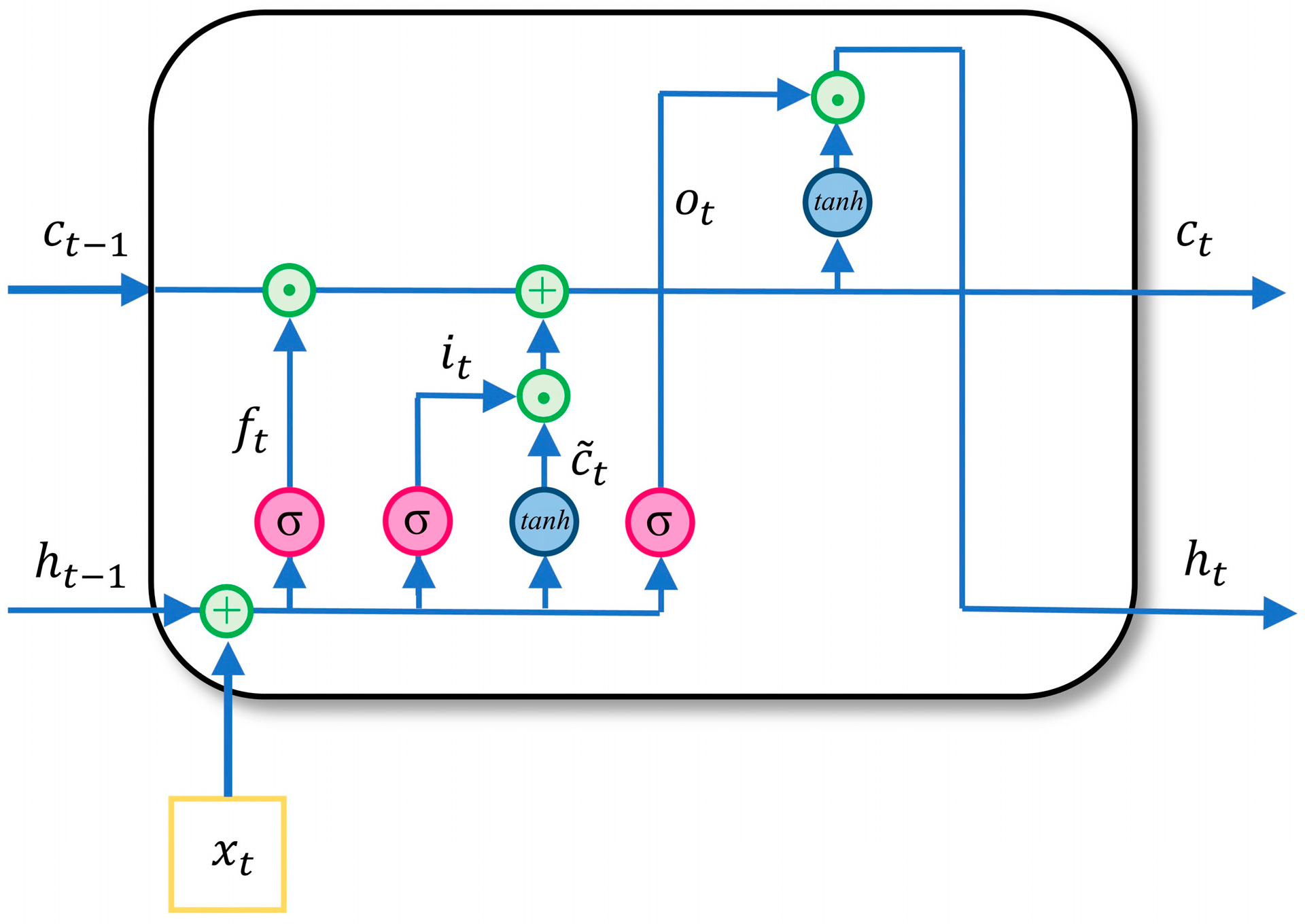
2.2. ConvLSTM Algorithm

ConvLSTM was first applied to the proximity forecasting of precipitation [34], which addresses the deficiency of LSTM in losing spatial correlation and spatial features of spatial data. ConvLSTM extracts feature from a series of images rather than from a single image. A model that processes sequential images needs to be able to extract spatial and temporal information from the images, as it should adapt to the changes in the sequential data over time. Thus, ConvLSTM uses convolution operations to generate a good spatial representation of each frame, using LSTM to encode the temporal variations in the sequence. The LSTM is a class of recurrent neural networks that can process sequential data and was introduced to solve the gradient disappearance problem encountered by recurrent neural networks when processing long sequences [31]. The LSTM incorporates memory units that contain information about the input seen by the LSTM units and is conditioned using several fully connected gates. Because the main purpose of processing image sequences is to discover changes in spatial and temporal dimensions, ConvLSTM uses convolutional gates in the LSTM to encode spatio-temporal information.

Equations (3)–(7) and Figure 1 describe the architecture of the ConvLSTM. The σ is the sigmoid function. The “∗” denotes the convolution operation and the “◦” denotes the Hadamard product. $i_t$ is the input gate, $f_t$ is the forgetting gate, $o_t$ is the output gate, $C_t$ is the current state, $H_t$ is the final output, and W, b represent the weight and bias coefficients, respectively, which are three-dimensional (3D) tensors. The ConvLSTM layer is a recursive layer, similar to the LSTM, except that the internal matrix multiplication is exchanged with the convolution operation. The data flow through the ConvLSTM unit keeps the input dimension as 3D and not just a one-dimensional vector. Thus, the ConvLSTM layer uses the same weight sharing as a CNN and treats the input data as serial data, which allows the model to process time-series data similar to an RNN.

$$i_t{=\mathsf{\sigma } (W}_{xi}{ \ast X}_t{+W}_{hi}{ \ast H}_{t-1}{+W}_{ci} ◦{ C}_{t-1}{+b}_i)$$

(3)

$$f_t{=\mathsf{\sigma } (W}_{xf}{ \ast X}_t{+W}_{hf}{ \ast H}_{t-1}{+W}_{cf} ◦{ C}_{t-1}{+b}_f)$$

(4)

$$C_t{=f}_t ◦{ C}_{t-1}{+i}_t ◦{\tanh (W}_{xc}{ \ast X}_t{+W}_{hc}{ \ast H}_{t-1}{+b}_c)$$

(5)

$$o_t{=\mathsf{\sigma } (W}_{xo}{ \ast X}_t{+W}_{ho}{ \ast H}_{t-1}{+W}_{co} ◦{ C}_t{+b}_o)$$

(6)

$$H_t{=o}_t ◦{ \tanh (C}_t)$$

(7)

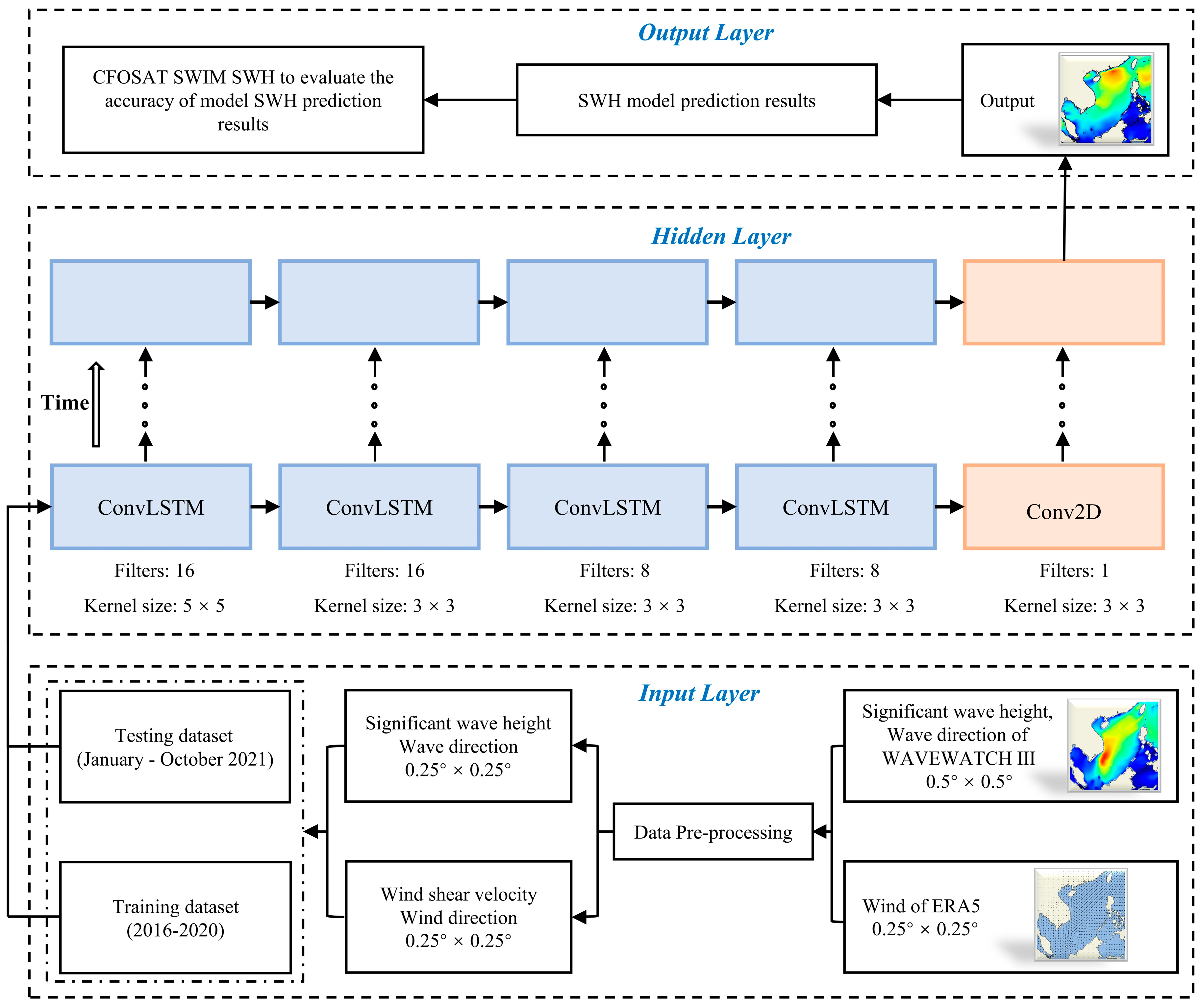
2.3. Constructing the SWH Prediction Model

Based on the ConvLSTM model for proximity precipitation forecasting by Shi et al. [34], a ConvLSTM model for SWH prediction in the SCS was developed in this study, and the overall structure of the model is shown in Figure 2. The model has five hidden layers for each step, including four ConvLSTM layers and one Conv2D layer as the final output layer. The process of the SWH forecast was to input several previous time data from each training set sample into the model of Figure 2 to obtain the SWH of the target time. The first SWH of WW3 and wind of ERA5 were initially 2D data; in the ConvLSTM algorithm, the traditional LSTM multiplication operation is transformed into convolution operation; it can directly operate on 2D data. In the final output, the SWH forecast can be directly output from the 2D map.

In this study, three different SWH prediction models for the SCS were established using SWH, U_*, Φ, and θ as the training and input data, respectively. Model A was built as a univariate SWH prediction model using only SWH as training and input data. The effect of two parameters, training dataset size and input data time span, on the forecasting effect of Model A was explored through 20 sets of sensitivity experiments. In these 20 experiments, the input data time span was chosen to be 2, 3, 4, and 5 h, and the training dataset size was opted to be 1, 2, 3, 4, and 5 years, respectively. The time span and training dataset size of the optimal input data were determined by analyzing and evaluating the error indices of twenty sets of experiments. In addition, wind speed and wind direction are also important physical factors affecting SWH. In order to further improve the accuracy of the prediction model, multi-variable input data were used to forecast SWH based on the Model A parameter settings. Model B was designed using SWH and U_* as input data, and Model C was constructed using SWH, U_*, Φ, and θ as input data. The three models developed in this study are as follows:

Model A:

$$H_p^{T+N}{=f (H}_w^T{, H}_w^{T-1}{, H}_w^{T-2})$$

(8)

Model B:

$$H_p^{T+N}{=f (H}_w^T{, H}_w^{T-1}{, H}_w^{T-2}{, U}_{\ast }^T{, U}_{\ast }^{T-1}{, U}_{\ast }^{T-2})$$

(9)

Model C:

$$H_p^{T+N}{=f (H}_w^T{, H}_w^{T-1}{, H}_w^{T-2}{, U}_{\ast }^T{\cos (\Phi }^T-{ \theta }^T{), U}_{\ast }^{T-1}{\cos (\Phi }^{T - 1}-{\theta }^T{), U}_{\ast }^{T-2}{\cos (\Phi }^{T - 2}-{\theta }^T\left)\right)$$

(10)

where T is a certain moment, T + N is the moment when the SWH needs to be predicted, $H_p$ denotes the SWH predicted by the model, $H_w$ denotes the SWH from WWIII.

2.4. Model Quality Assessment Methods

To quantify the accuracy of the SWH prediction model, model quality was assessed using root mean square error (RMSE), correlation coefficient (CC), and mean absolute percentage error (MAPE), with expressions as shown in Equations (11) to (13).

$$\mathit{RMSE}=\sqrt{ \frac{1}{M}{\sum }_{i=1 }^M{{(H}_p-H_w)}^2}$$

(11)

$$CC=\frac{\frac{1}{M}{\sum }_{i=1}^M\left(\left(H_p-{\overline{H}}_p\right)\left(H_w-{\overline{H}}_w\right)\right)}{\sqrt{\frac{1}{M}{\sum }_{i=1}^M{\left(H_p-{\overline{H}}_p\right)}^2}·\sqrt{\frac{1}{M}{\sum }_{i=1}^M{\left(H_w-{\overline{H}}_w\right)}^2}}$$

(12)

$$\mathit{MAPE}=\frac{1}{M}{{\displaystyle \sum }}_{i=1 }^M\frac{\left|H_p-H_w\right|}{H_w} \times 100\%$$

(13)

where M is the total number of cases, $H_p$ represents the predicted SWH, $H_w$ represents the SWH from WWIII, ${\overline{H}}_w$ represents the average of WWIII, and ${\overline{H}}_p$ represents the average of the predicted SWH. Since the CFOSAT data have spatial and temporal discontinuities, therefore, in the training and test sets of the SWH prediction model, the SWH of WWIII, which was validated by CFOSAT data, was used in this study to calculate the RMSE, MAPE, and CC of the predicted data.

To evaluate the discrepancy in the prediction performance of different models, in Equation (14), the assessment skill used by Ji et al. [49] with corresponding changes based on this study was used to assess the numerical differences in the error indices among the models.

$$\mathit{Skill}{ }_{\mathit{index}}^{a b}=\frac{\left|{ E}_{ \mathit{index}}^{ m a}-E_{ \mathit{index}}^{ m b} \right|}{E_{ \mathit{index}}^{ m a}}\times 100\%$$

(14)

where $E_{ \mathit{index}}^{ m a}$ and $E_{ \mathit{index}}^{ m b}$ denote the values of the error indices of model a and model b, respectively, and “index” denotes the different error indices of the models, including RMSE, CC, and MAPE.

3. Results and Discussion

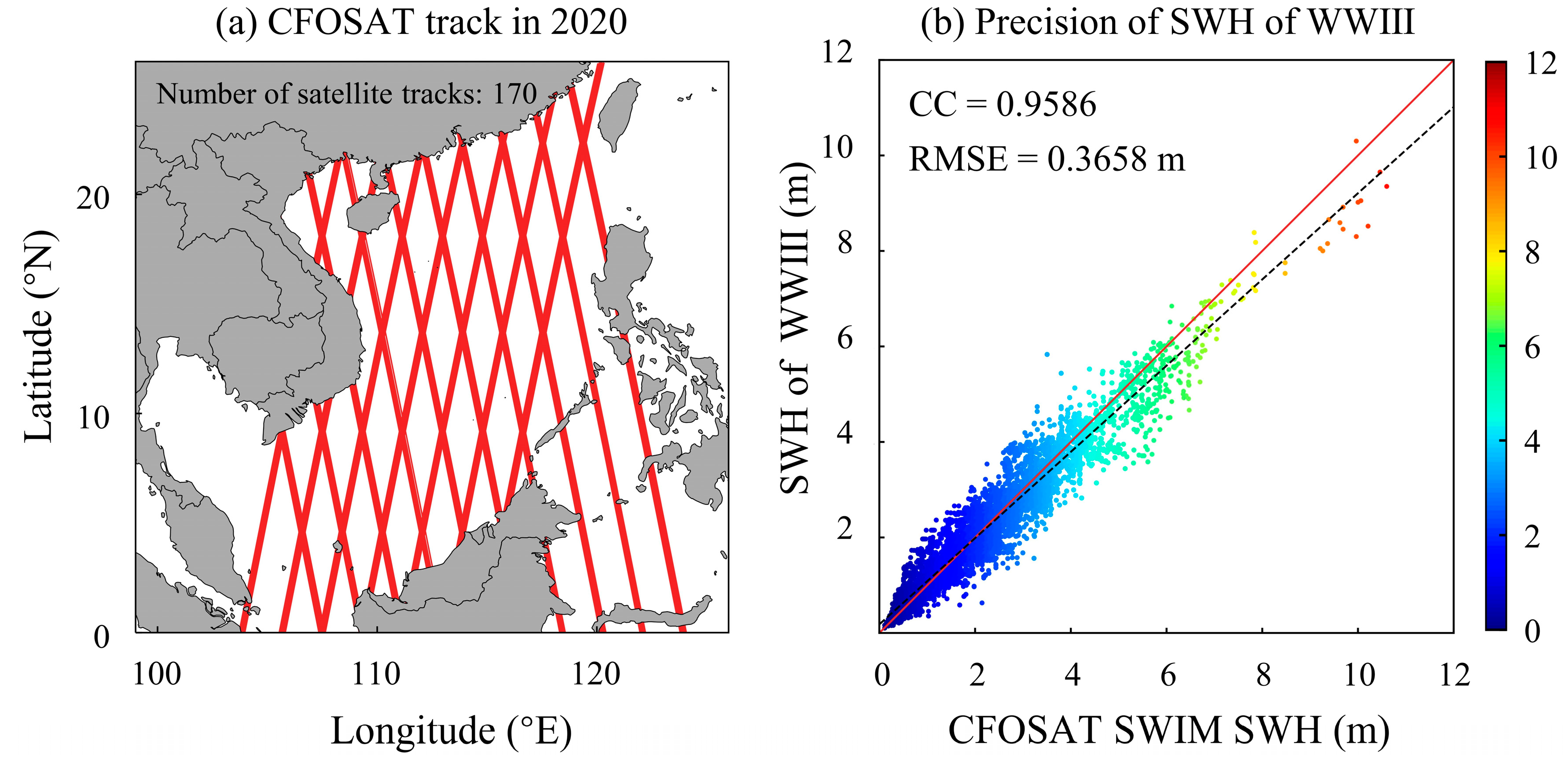
3.1. Validation of SWH from WWIII

The SWH from WWIII from PacIOOS was evaluated by the SWH from satellite. Li et al. [46] demonstrated that CFOSAT can provide high-precision SWH. Thus, the study used CFOSAT SWIM SWH to calculate the SWH from WWIII for CC and RMSE (Figure 3b). Altogether, 170 CFOSAT tracks of SWH data in 2020 (Figure 3a) were collected in the study to evaluate the SWH data of the training set in 2020. Compared with the CFOSAT SWIM SWH, the CC of SWH from WWIII is 0.9586 and the RMSE is 0.3658 m in 2020 (Figure 3b). Therefore, the precision of the SWH from WWIII is within a certain extent that is acceptable and can be used as the training data for the SWH prediction model.

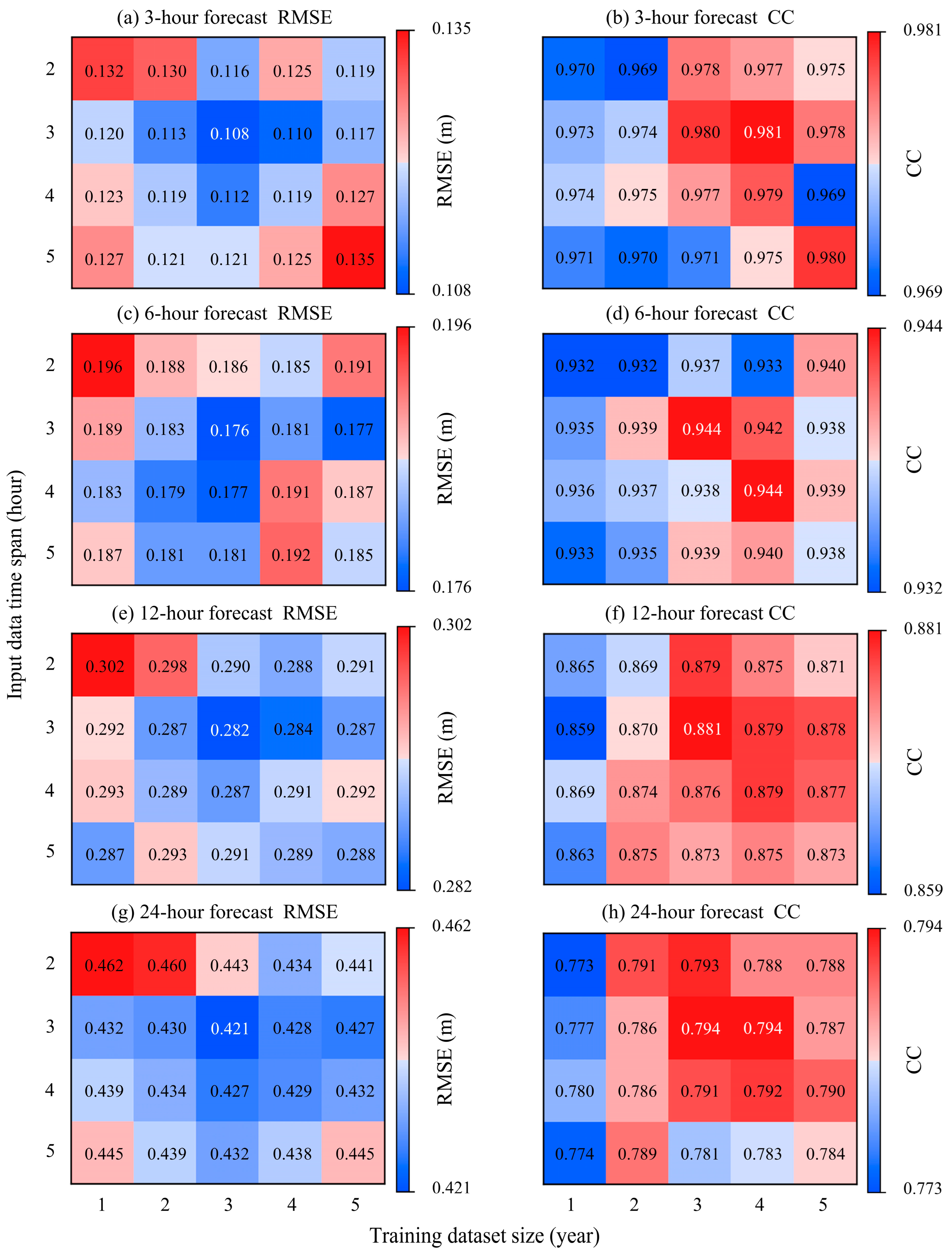
3.2. Model A Sensitivity Experiments

Model A was built using only SWH as training and input data for the SWH prediction model in the SCS. In the process of establishing Model A, because the training dataset size and the input data time span were critical parameters affecting the performance of the forecast model, the effects of these two parameters on the forecasting effectiveness of Model A were explored through 20 sensitivity experiments. The time range of the training set chosen for the experiments was from 2016 to 2020, and the time range of the validation set was from January to October 2021. The RMSE and CC were used in these experiments to assess the performance differences between different experimental models. Figure 4 shows the RMSE and CC results of SWH forecasting at 3-, 6-, 12-, and 24-h for the twenty sets of experiments, respectively.

For a fixed input data time span, each row in Figure 4 shows the relationship between the experimental model’s RMSE, CC, and the training dataset size. As the training dataset size increases, the experimental model has the characteristics that the RMSE decreases at first and increases after, and CC ascends and then diminishes. At a specific training dataset size, each column in Figure 4 shows the relationship between the RMSE, CC, and the experimental model’s input data time span. As the input data time span increases, the RMSE of the experimental model first decreases and then increases, and CC first ascends and then diminishes.

With a constant training dataset size, the model with a time span of 3 h had the smallest RMSE and the highest CC in the 3- (Figure 4a,b), 12- (Figure 4e,f), and 24-h (Figure 4g,h) SWH forecasting; the model with a time span of 3 or 4 h had the smallest RMSE and the largest CC in the 6-h (Figure 4c,d) SWH forecasting. When the input data time span was 2 h, the forecasting accuracy was low due to the small amount of wave data. As the time span rises, the CC of the model gradually increases, and RMSE decreases by degrees. However, when the input data time span was too large, the precision of model did not further improve due to the data’s redundancy. For the experiments with a determined time span of input data, the experimental model with a training dataset size of 3 years had the smallest RMSE and the highest CC for SWH forecasting of 3- (Figure 4a,b), 6- (Figure 4c,d), and 24-h (Figure 4g,h); for SWH forecasting of 12-h (Figure 4e,f), the experimental model with a training dataset size of 3 or 4 years had the lowest RMSE and the largest CC. As training dataset size increases, the CC of the model gradually advances, and the RMSE decreases by degrees. However, after the training dataset size was greater than 3 years, the increase in model accuracy was not apparent, but the model consumed significantly more computer resources.

We considered the model quality of the SCS SWH prediction model and the computational resources consumed when training the model. Concerning SCS SWH forecasting for 3-, 6-, 12- and 24-h, compared with other experimental models, the model at this moment predicted SWH with not only the smallest RMSE but also the largest CC when the input data time span was 3 h and the training dataset size was 3 years. The RMSE of the model were 0.108 m, 0.176 m, 0.282 m, and 0.421 m, and CC were 0.980, 0.944, 0.881, and 0.794, respectively. These parameters were the optimal prediction model parameters. Therefore, the same parameter settings were adopted in Model B and C.

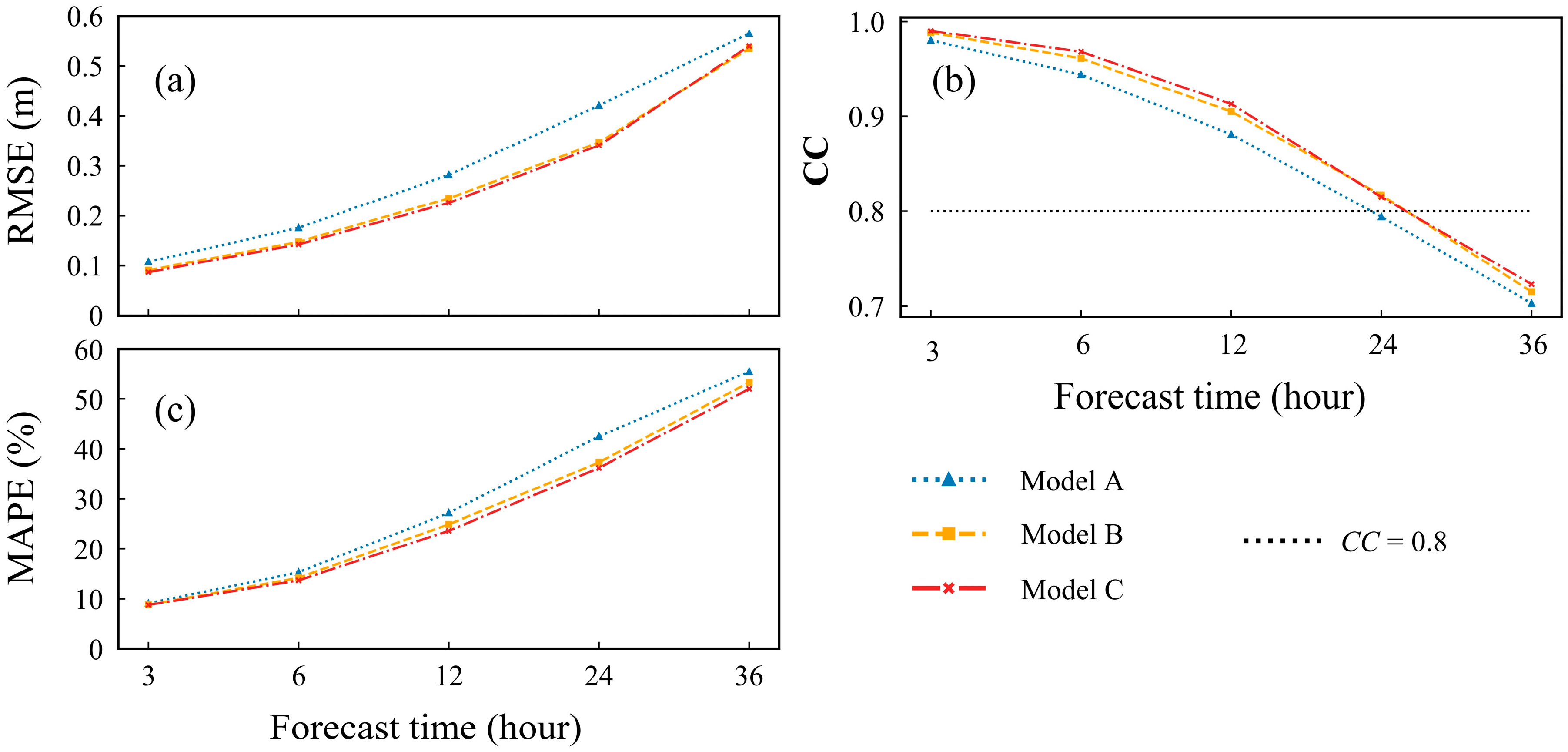
3.3. Model Comparison and Analysis

Model A, B, and C were used to predict SWH at 3-, 6-, 12-, 24-, and 36-h in the SCS. In order to compare the performance of the models, the error statistics of the three models were calculated, and the root mean square error (RMSE), correlation coefficient (CC), and mean absolute percentage error (MAPE) were calculated, respectively. Figure 5 shows the error indices variation curves for the three models for 3-, 6-, 12-, 24-, and 36-h SWH forecasting on the test set. The blue dashed line, orange dashed line, and red dashed line represent Model A, B, and C, respectively. As shown in the figure, the RMSE (Figure 5a) and MAPE (Figure 5c) of the prediction model gradually increase and CC (Figure 5b) gradually decreases as the forecasting time increases from 3-h to 36-h. This was consistent with the theory and the expected result. Meanwhile, as shown in Figure 5, for the 3-h SWH forecast, the RMSE and MAPE of Model A, B, and C were fewer and the CC between the predicted SWH and the SWH from WWIII was large. For a fixed forecast time, the RMSE and MAPE of Model B were less than those of Model A, and the CC of Model B was larger than that of Model A. This was because the accuracy of the models depends not only on the wave parameters but also on the previous wind speed. Model C outperforms Model B for the 3-, 6-, and 12-h SWH forecasts, but for the 24-h SWH forecast, the differences in RMSE, MAPE, and CC between Model C and Model B were very small. Particularly, the RMSE of Model C was rather slightly larger than Model B for the 36-h forecast. The result means that for lengthy forecasts (36 h or more), wind and wave directions had a very weak impact on forecast performance. It may even cause a reduction in forecast accuracy due to data redundancy. In addition, as shown in Figure 5b, the CC of Model B and Model C were greater than 0.8 for the 24-h SWH forecast (0.817 and 0.815, respectively), and the forecast results were considered to be significantly correlated with the true values at this time. Therefore, for our study, we focused on the SWH forecast results over a 24-h time period. The comprehensive assessment showed that for SWH prediction within 24 h, Model C outperforms other models in terms of integrated predictive capability.

In order to further quantify the impact of multi-element training and input data on model performance, evaluations of the changes in RMSE, CC, and MAPE from Model A to Model B to Model C were performed. The statistical analysis of the $\mathit{Skill}{ }_{\mathit{index}}^{A B}$ and $\mathit{Skill}{ }_{\mathit{index}}^{A C}$ was completed in

Table 2. Error indices improvement (Skill) of Model B and Model C relative to Model A.

Forecast Time	Skill	3-h	6-h	12-h	24-h
RMSE	$\mathit{Skill}{ }_{\mathit{RMSE}}^{A B}$ (%)	15.7	15.9	16.7	17.6
	$\mathit{Skill}{ }_{\mathit{RMSE}}^{A C}$ (%)	19.4	18.8	19.9	19.0
CC	$\mathit{Skill}{ }_{\mathit{CC}}^{A B}$ (%)	0.82	1.80	2.72	2.90
	$\mathit{Skill}{ }_{\mathit{CC}}^{A C}$ (%)	1.02	2.54	3.63	2.65
MAPE	$\mathit{Skill}{ }_{\mathit{MAPE}}^{A B}$ (%)	3.40	7.19	8.46	12.2
	$\mathit{Skill}{ }_{\mathit{MAPE}}^{A C}$ (%)	3.84	10.5	13.2	14.8

based on the error indices of each model in Figure 5 and Equation (14). According to the results in Table 2, for the 3-h SWH forecast, both $\mathit{Skill}{ }_{\mathit{index}}^{A B}$ and $\mathit{Skill}{ }_{\mathit{index}}^{A C}$ were relatively small and gradually increased with the increase in forecasting time. Both $\mathit{Skill}{ }_{\mathit{index}}^{A B}$ and $\mathit{Skill}{ }_{\mathit{index}}^{A C}$ were larger for the 6- and 12-h SWH forecast. However, the discrepancies between $\mathit{Skill}{ }_{\mathit{index}}^{A B}$ and $\mathit{Skill}{ }_{\mathit{index}}^{A C}$ were not significant for the 24-h SWH forecast. When the forecast time was relatively longer (6- and 12-h), the results of Model A were less accurate compared with the results of Model B and C. When the forecast time was too long (24-h) or too short (3-h), the input of multiple elements did not significantly improve the forecast performance. This was because the correlation between wave height and previous wave/wind characteristics became lower at longer forecast times [37]. The $\mathit{Skill}{ }_{\mathit{index}}^{A C}$ was greater than $\mathit{Skill}{ }_{\mathit{index}}^{A B}$ with respect to a fixed forecasting time.

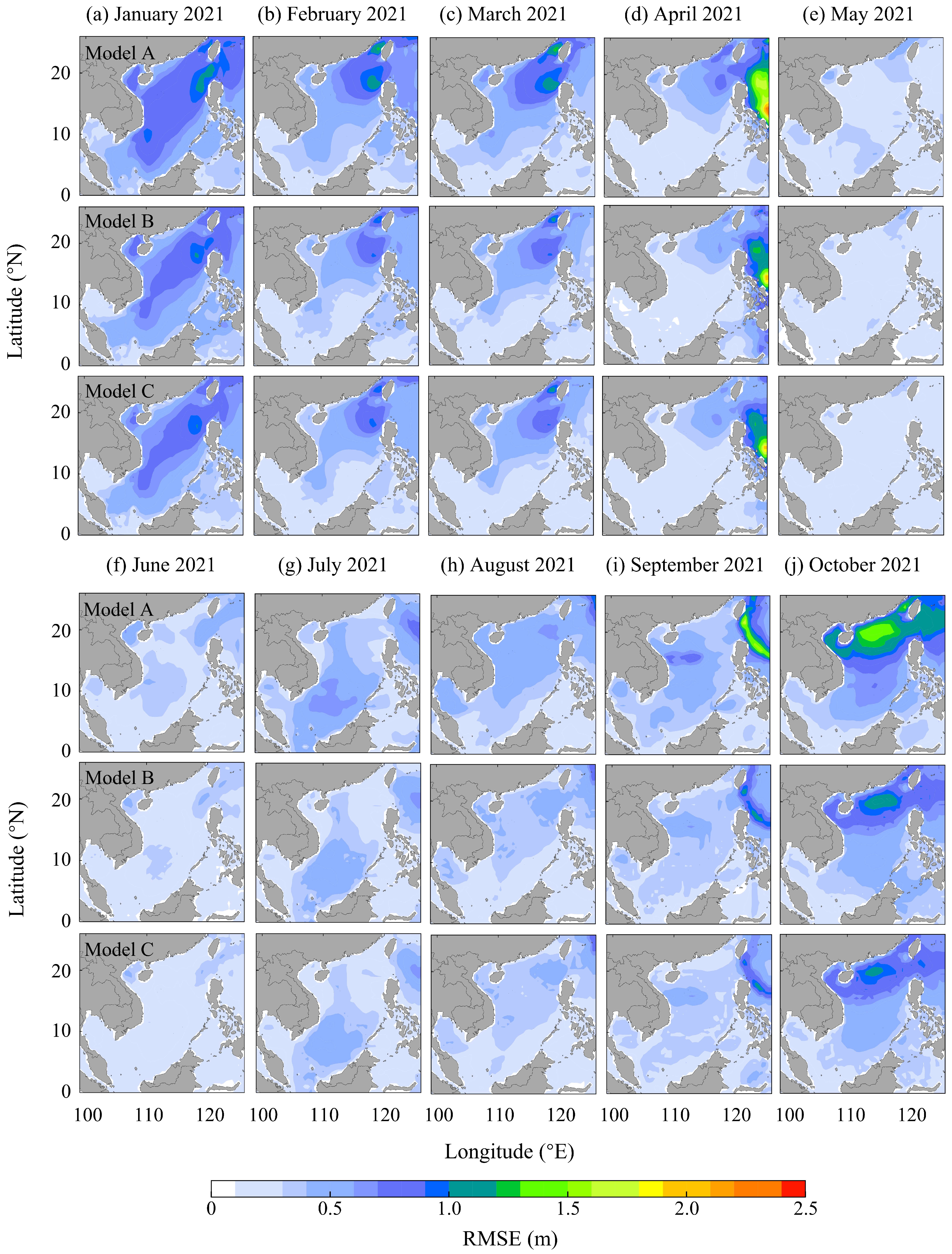
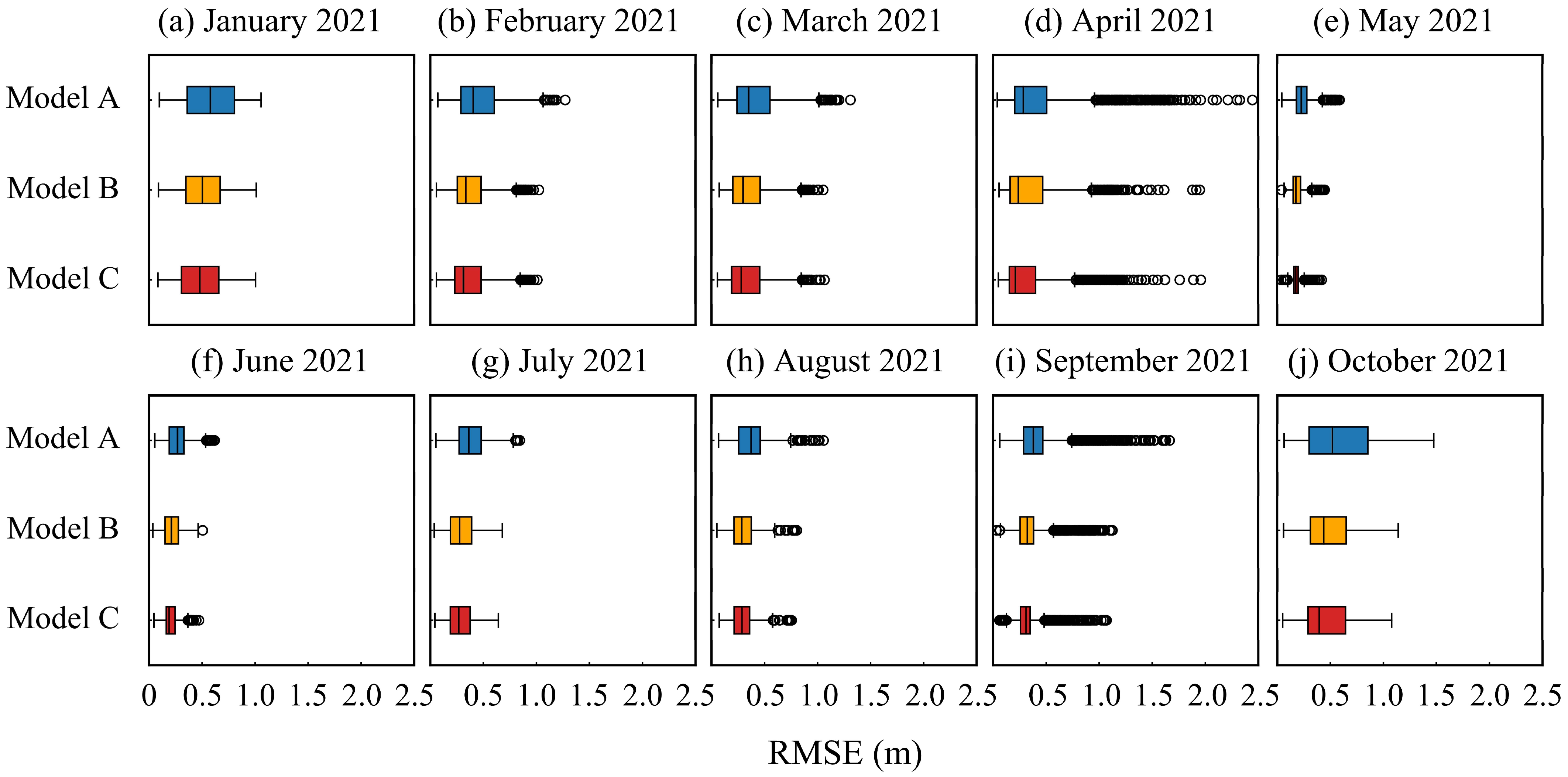
3.4. Spatial Distribution and Statistical Analysis of Model Errors

To evaluate the spatio-temporal distribution characteristics of the model errors of SWH forecasts in the SCS, Figure 6 shows the spatial distribution results of the monthly mean RMSE of Model A, B, and C in the 24-h SWH forecast from January to October 2021. The RMSE and spatial locations of all three SCS SWH forecast models were significantly correlated, with smaller RMSE in the deep-sea region away from the coast yet larger RMSE in the shallow-water region along the coast. This was because wind–wave relationships in the nearshore shallow water area are uncertain due to irregular shoreline shapes and seafloor conditions, while the interaction of ocean hydrodynamics and coastal morphology leads to complex relationships between wind and waves [47]. In addition, the RMSE of the prediction models was relatively larger in the eastern and southeastern parts of the SCS, which might be due to multiple reasons. SWH from WWIII was used as the training data, and the error of the prediction results was affected by the accuracy of the original data. Meanwhile, the frequent typhoon events in the sea near the Luzon Strait [5,6] cause irregular and drastic changes in SWH in the nearby ocean. It is difficult for the prediction model to obtain information on the spatial and temporal characteristics of SWH. In addition, many islands are in the eastern and southeastern parts of the SCS, resulting in spatial incoherence of wave data. The lack of data information may also be the reason for this phenomenon. Moreover, the monthly mean RMSE of the SWH prediction model had monthly variations. The prediction model had the smallest RMSE for May–August 2021, followed by the results for January–March 2021, and the worst forecasting for April, September, and October 2021 with the largest RMSE.

In order to quantitatively evaluate the magnitude of the monthly mean RMSE of Model A, B, and C in the 24-h SCS SWH forecast, the results of the spatial distribution of RMSE in Figure 6 were statistically analyzed, and boxplots of RMSE statistics were plotted (Figure 7). As shown in Figure 7, each subplot’s blue, red, and orange boxes indicate the RMSE statistics of Model A, B, and C. From Model A to Model B to Model C, the median and third quartile of the models were decreasing, and it can be observed that in most months, the median and third quartile of Model C were the minimum. Model C had the best forecasting ability. Meanwhile, the RMSE of the prediction model had the most outliers in April and September 2021 (Figure 7d,i), indicating that the RMSE of the model had more exception value in these two months.

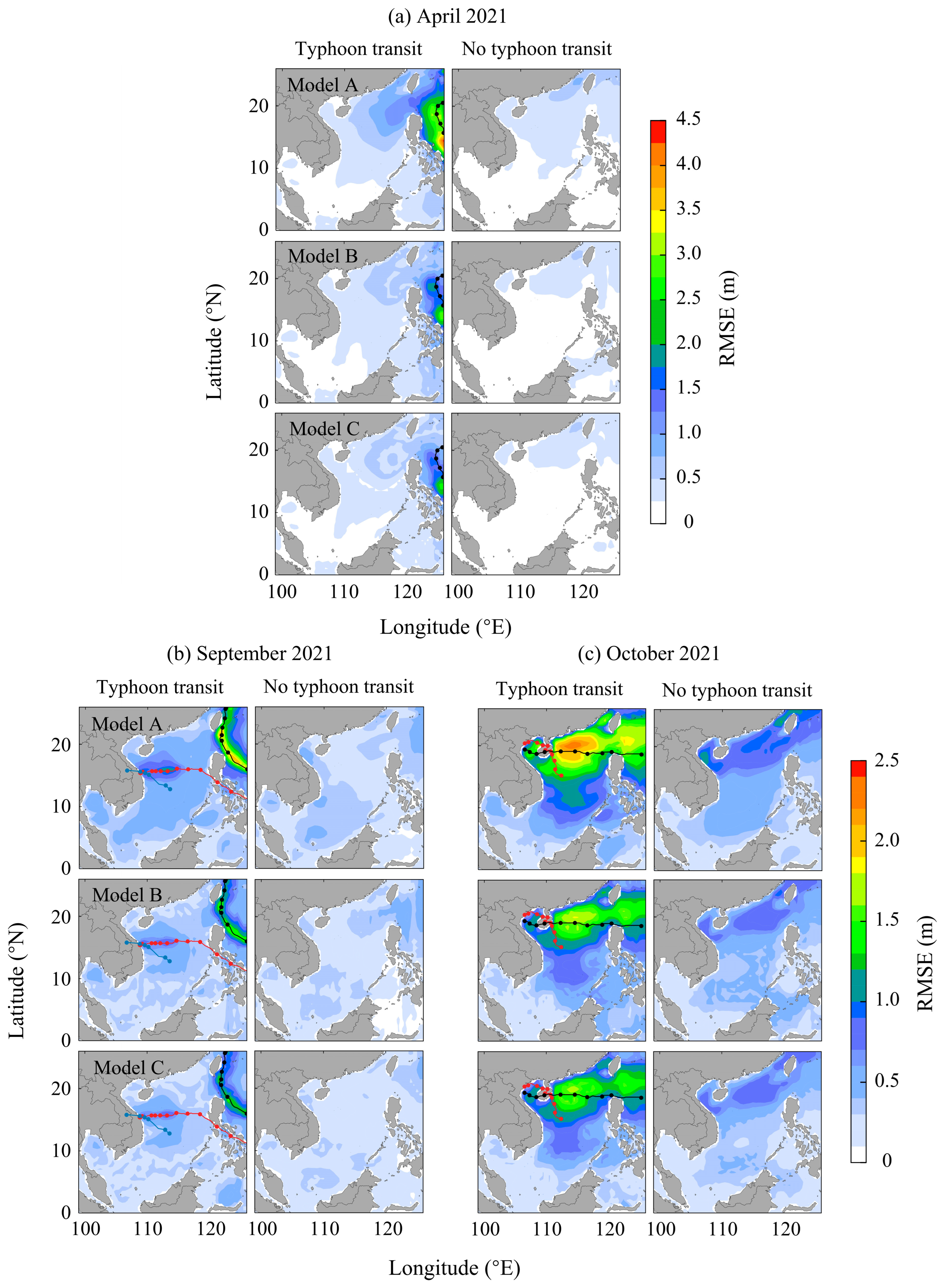
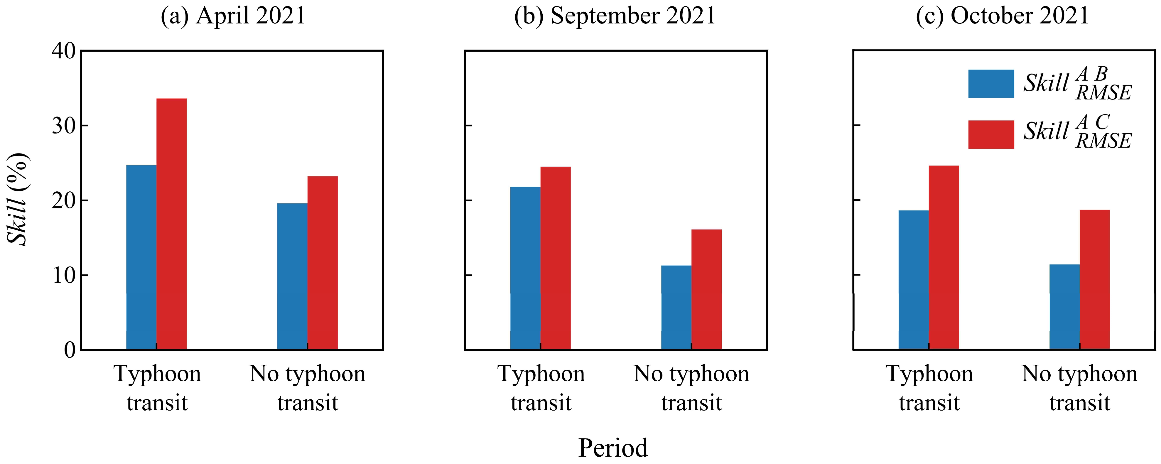
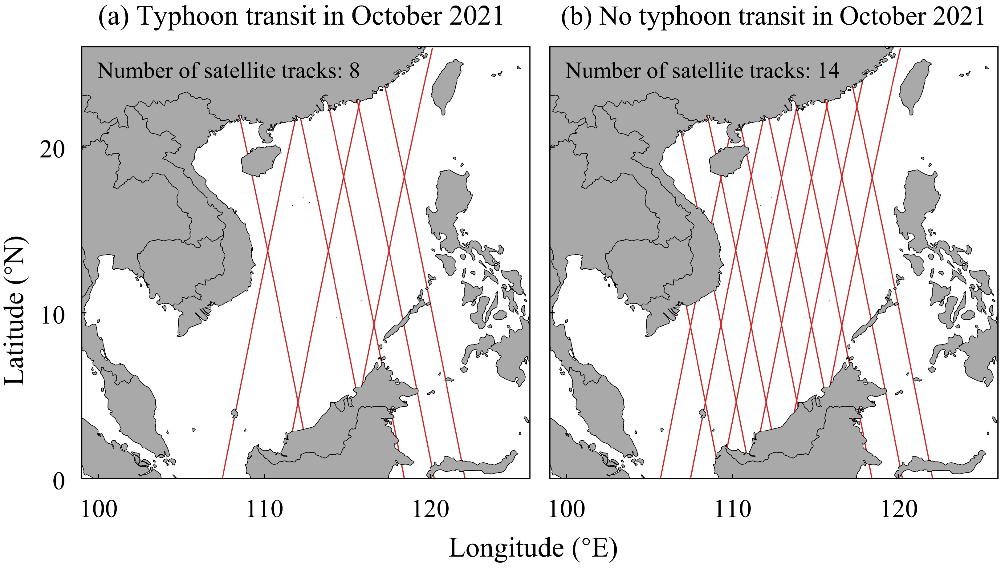
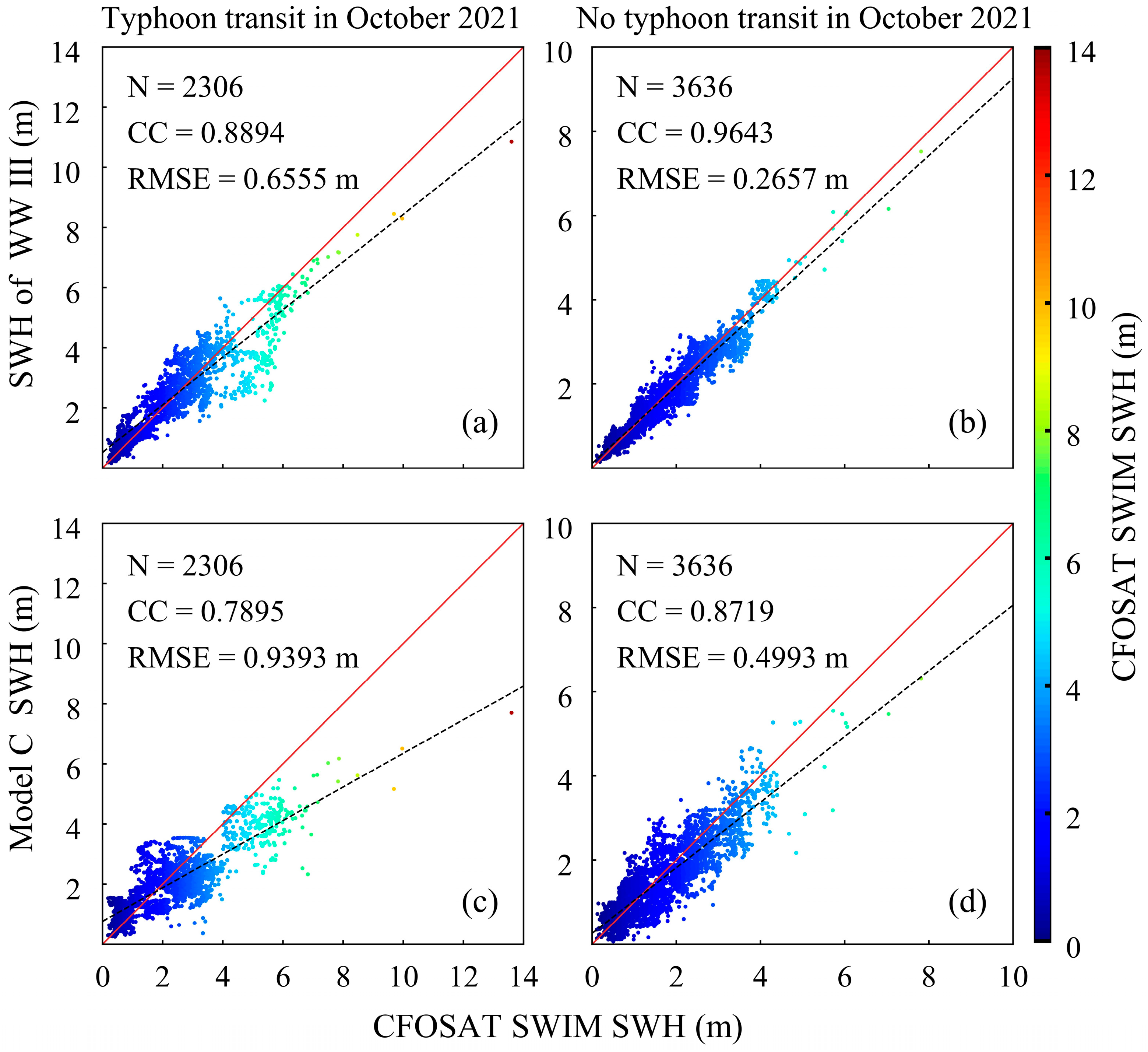
3.5. Model Performance in Extreme Weather

Figure 6 and Figure 7 show that the prediction model had maximum values and more outliers for the RMSE results in April, September, and October 2021. Based on the information on generated or transiting typhoons and tropical storms for April, September, and October 2021 in the SCS waters in Table 1, the spatial distribution characteristics of the RMSE of the prediction model under extreme weather conditions were analyzed. For April, September, and October 2021, the spatial distribution of the RMSE of the prediction model was calculated by dividing each month into two periods with typhoon transit and no typhoon transit, respectively. Figure 8 shows the spatial distribution of RMSE in the 24-h SWH forecast for the three months mentioned above. The left and right plots in each subplot indicate the presence and absence of typhoon transit, respectively, where the solid line in the left plot indicates the typhoon path in that month. The solid black line in Figure 8a is the path of Typhoon 2102 “Surigae”. The solid red, black and blue lines in Figure 8b are the paths of Typhoon 2113 “Conson”, Typhoon 2114 “Chanthu” and Typhoon 2115 “Dianmu”, respectively. The solid red and black lines in Figure 8c are the paths of Typhoon 2117 “Lionrock” and Typhoon 2118 “Kompasu”, respectively.

As shown in Figure 8, there is a close spatial correlation between the spatial distribution of RMSE during the occurrence of typhoons and the path of typhoons in each month, and the RMSE of the prediction models is small during the periods when there is no typhoon transit. This is consistent with the findings in Figure 8 that wind resistance coefficients in extreme conditions were very different from those in weak wind conditions, which may alter the relationship between wind and waves and, thus, reduce the accuracy of predicting extreme events [50]. Meanwhile, the RMSE changes between the three models with and without typhoon transit were compared separately. In the period with typhoon transit, the RMSE of Model B and C, constructed by adding wind field data to the input data, decreased significantly compared to Model A’s. The RMSE changes in Model B and C compared to those in Model A in the period without typhoon transit were insignificant.

In order to quantitatively analyze this feature, according to Equation (14), the ${\mathit{Skill} }_{\mathit{RMSE}}^{A B}$ and ${\mathit{Skill} }_{\mathit{RMSE}}^{A C}$ of typhoon transit or no typhoon transit were statistically analyzed in Figure 9. The left and right histograms in each subplot denote the presence and absence of typhoon transit, respectively, and the blue and red histograms indicate ${\mathit{Skill} }_{\mathit{RMSE}}^{A B}$, and ${\mathit{Skill} }_{\mathit{RMSE}}^{A C}$, respectively. As shown in Figure 9, the ${\mathit{Skill} }_{\mathit{RMSE}}^{A B}$ and ${\mathit{Skill} }_{\mathit{RMSE}}^{A C}$ for each month of the typhoon transit period in April, September, and October 2021, with extreme weather occurrences, were greater than that for the period without typhoon transit. It indicates that the quality of the prediction models and the wind field were more correlated in the period with extreme weather occurrences. At the same time, the ${\mathit{Skill} }_{\mathit{RMSE}}^{A C}$ was bigger than the ${\mathit{Skill} }_{\mathit{RMSE}}^{A B}$.

In order to quantify this feature more coherently, the ${\mathit{Skill} }_{\mathit{RMSE}}^{A B}$ and ${\mathit{Skill} }_{\mathit{RMSE}}^{A C}$ for typhoon transit or no typhoon transit in April, September, and October 2021 were calculated in

Table 3. Mean of $\mathit{Skill}{ }_{\mathit{RMSE}}^{A B}$ and ${\mathit{Skill} }_{\mathit{RMSE}}^{A C}$ for typhoon transit or no typhoon transit in April, September, and October 2021.

Periods	${\mathit{Skill} }_{\mathit{RMSE}}^{\mathit{A} \mathit{B}}$ (%)	${\mathit{Skill} }_{\mathit{RMSE}}^{\mathit{A} \mathit{C}}$ (%)
Typhoon transit	21.7	27.5
No typhoon transit	14.1	19.3

. As shown in Table 3, the best performance for Model C was constructed using SWH, wind shear velocity, wind direction, and wave direction data.

For validation of the accuracy of Model C in the 24-h SWH forecasting and further comparison of the accuracy characteristics of the model during typhoon transit and no typhoon transit, we obtained CFOSAT SWIM SWH data products provided by AVISO+. As shown in Figure 8, typhoons had the largest impact in the SCS in October 2021. Therefore, we selected 22 tracks of CFOSAT SWIM SWH data that passed through SCS in October 2021, including 8 tracks during the typhoon (Figure 10a) and 14 tracks during no typhoon transit period (Figure 10b).

The SWH from WWIII and Model C SWH were interpolated to the coordinates corresponding to the tracks data by the nearest neighbor method. The quality of the original SWH from WWIII data during typhoon and no typhoon were analyzed first (Figure 11a,b). Subsequently, we analyzed the accuracy characteristics of Model C in the 24-h SWH forecasting during typhoon transit and no typhoon transit period by correlation and error analysis (Figure 11c,d). During typhoon transit, the CC of SWH from WWIII relative to CFOSAT SWIM SWH was 0.8894 and the RMSE was 0.6555 m (Figure 11a); during no typhoon transit, the CC of SWH from WWIII relative to CFOSAT SWIM SWH was 0.9643 and the RMSE was 0.2657 m (Figure 11b). In the 24-h SWH forecasting, the CC of Model C SWH relative to CFOSAT SWIM SWH was 0.7895 and RMSE was 0.9393 m during typhoon transit (Figure 11c); during no typhoon transit, the CC of Model C SWH relative to CFOSAT SWIM SWH was 0.8719 and RMSE was 0.4993 m (Figure 11d).

In summary, the prediction precision of Model C during typhoon transit was not as accurate as that during no typhoon transit for the 24-h SWH forecasting. There were probably two reasons. One was that the accuracy of SWH from WWIII during typhoon transit is comparatively less, and the input data influenced the accuracy of Model C forecasting SWH. Another reason was that during the no typhoon transit period, it was more difficult for Model C to encompass the characteristic patterns of the wave and wind fields during the drastic changes, which then contributed to the decrease of the predicted SWH accuracy.

4. Conclusions

In this study, in order to explore the role of discrepancy input elements in the ConvLSTM algorithm-based SWH prediction in the South China Sea, three different prediction models were developed using SWH, wind shear velocity (U_*), wind direction (Φ), and wave direction (θ) as input data. Model A was constructed using single-element (SWH) training and input data. The two important parameters of input data time span and training dataset size were determined by sensitivity experiments. To further improve the performance of the SWH forecasting model, Model B and C were constructed using multi-element training and input data. Model B used SWH and U_* data to predict SWH, and Model C added wind and wave direction data to the input data of Model B. Subsequently, the spatial distribution characteristics and differences of the forecast results of the three models were analyzed, and the forecast characteristics and discrepancies of the three models under extreme climate were discussed.

The main innovation of this paper was to consider the influence of various physical factors on the prediction model in the prediction of 2-dimensional SWH field. The effect of wind forcing on SWH was quantified using wind shear velocity instead of wind speed, especially the use of cos (Φ − θ) to quantify the influence of the difference between wind and wave directions for the SWH. Moreover, the relationship between the prediction model performance and the typhoon tracks was explored.

The most significant findings of this study are as follows: It is feasible to apply the ConvLSTM algorithm to the forecast of SWH in the South China Sea, which can provide an efficient and high-precision forecast of SWH. When using only the SWH data as input data to predict the SWH in the South China Sea, the optimal training dataset size for the model was 3 years, and the optimal input data time step was 3 h. Model C, in which the SWH, U_*, and cos (Φ − θ) were conducted as input data, outperformed other models. For the 3-h SWH forecasting, the correlation between the forecasting results and the wind field was not significant. For the 6- and 12-h SWH forecast, the ${\mathit{Skill} }_{\mathit{RMSE}}^{A C}$ gradually increased when U_* and cos (Φ − θ) were added to the input data. However, the discrepancies between ${\mathit{Skill} }_{\mathit{index}}^{A B}$ and ${\mathit{Skill} }_{\mathit{index}}^{A C}$ were not significant for the 24-h SWH forecast.

The RMSE of the SWH prediction models had spatial distribution characteristics, and the RMSE of the models was smaller in the deep-water region far from the shore. However, the RMSE of the models was larger in the shallow water region along the coast. The RMSE of the SWH prediction models and the extreme climate were spatially and temporally correlated, and the RMSE of the models was larger in the vicinity of the typhoon path during the period of typhoon occurrence. In addition, ${\mathit{Skill} }_{\mathit{RMSE}}^{A C}$ was 27.5% for the period of typhoon transit and 19.3% for the period of no typhoon transit, which implies that the correlation between SWH and the previous U_*, Φ, and θ was greater during the period of typhoon transit. As the training data show larger error during the period of typhoon transit than that without typhoon, Model C also showed a similar performance in forecasting error as SWH from WWIII.

There were several potential points for improvement in this study. When using multi-element training and input data, the optimal input data time span and training dataset size for Model B and C probably differ from the parameter values that were identified in Model A. This would necessitate further discussion in subsequent work. In addition, the achievement of this study was limited to the SWH prediction, and more diverse physical elements can be added as training and input data in the subsequent work to achieve multi-element prediction, such as simultaneous prediction of wave direction and average wave period, etc.

References

1. Wu, L.; Li, X.; Wu, T. South China Sea wave height trends analysis using 20CR reanalysis. In Proceedings of the 2016 International Conference on Automatic Control and Information Engineering, Hong Kong, China, 22–23 October 2016; pp. 57–61. [Google Scholar]
2. Sun, Z.; Zhang, H.; Xu, D.; Liu, X.; Ding, J. Assessment of wave power in the South China Sea based on 26-year high-resolution hindcast data. Energy 2020, 197, 117218. [Google Scholar] [CrossRef]
3. Zhang, Y.; Zhou, W.; Leung, M.Y.T. Phase relationship between summer and winter monsoons over the South China Sea: Indian Ocean and ENSO forcing. Clim. Dyn. 2018, 52, 5229–5248. [Google Scholar] [CrossRef]
4. Chen, X.; Wang, Y.; Zhao, K.; Wu, D. A Numerical Study on Rapid Intensification of Typhoon Vicente (2012) in the South China Sea. Part I: Verification of Simulation, Storm-Scale Evolution, and Environmental Contribution. Mon. Weather Rev. 2017, 145, 877–898. [Google Scholar] [CrossRef]
5. Wang, J.; Liu, J.; Wang, Y.; Liao, Z.; Sun, P. Spatiotemporal variations and extreme value analysis of significant wave height in the South China Sea based on 71-year long ERA5 wave reanalysis. Appl. Ocean Res. 2021, 113, 102750. [Google Scholar] [CrossRef]
6. Wu, Z.; Chen, J.; Jiang, C.; Deng, B. Simulation of extreme waves using coupled atmosphere-wave modeling system over the South China Sea. Ocean Eng. 2021, 221, 108531. [Google Scholar] [CrossRef]
7. Sverdrup, H.U.; Munk, W.H. Wind, Sea and Swell: Theory of Relations for Forecasting; Hydrographic Office: Taunton, UK, 1947. [Google Scholar]
8. Neumann, G.; Pierson, W.J. A detailed comparison of theoretical wave spectra and wave forecasting methods. Dtsch. Hydrogr. Z. 1957, 10, 134–146. [Google Scholar] [CrossRef]
9. Kamranzad, B.; Etemad-Shahidi, A.; Kazeminezhad, M.H. Wave height forecasting in Dayyer, the Persian Gulf. Ocean Eng. 2011, 38, 248–255. [Google Scholar] [CrossRef] [Green Version]
10. Wamdi, G. The WAM model—A third generation ocean wave prediction model. J. Phys. Oceanogr. 1988, 18, 1775–1810. [Google Scholar] [CrossRef]
11. Booij, N.; Ris, R.C.; Holthuijsen, L.H. A third-generation wave model for coastal regions: 1. Model description and validation. J. Geophys. Res. Oceans 1999, 104, 7649–7666. [Google Scholar] [CrossRef] [Green Version]
12. Rogers, W.E.; Hwang, P.A.; Wang, D.W. Investigation of wave growth and decay in the SWAN model: Three Regional-Scale applications. J. Phys. Oceanogr. 2003, 33, 366–389. [Google Scholar] [CrossRef]
13. Tolman, H.L. User Manual and System Documentation of WAVEWATCH III Version 3.14. 2009. Available online: https://polar.ncep.noaa.gov/mmab/papers/tn276/MMAB_276.pdf (accessed on 8 December 2021).
14. Mentaschi, L.; Besio, G.; Cassola, F.; Mazzino, A. Performance evaluation of WAVEWATCH III in the Mediterranean Sea. Ocean Model. 2015, 90, 82–94. [Google Scholar] [CrossRef]
15. Etemad-Shahidi, A.; Mahjoobi, J. Comparison between M5′ model tree and neural networks for prediction of significant wave height in Lake Superior. Ocean Eng. 2009, 36, 1175–1181. [Google Scholar] [CrossRef]
16. Wang, W.; Tang, R.; Li, C.; Liu, P.; Luo, L. A BP neural network model optimized by mind evolutionary algorithm for predicting the ocean wave heights. Ocean Eng. 2018, 162, 98–107. [Google Scholar] [CrossRef]
17. Deshmukh, A.N.; Deo, M.C.; Bhaskaran, P.K.; Balakrishnan Nair, T.M.; Sandhya, K.G. Neural-Network-Based data assimilation to improve numerical ocean wave forecast. IEEE J. Ocean. Eng. 2016, 41, 944–953. [Google Scholar] [CrossRef]
18. Mafi, S.; Amirinia, G. Forecasting hurricane wave height in Gulf of Mexico using soft computing methods. Ocean Eng. 2017, 146, 352–362. [Google Scholar] [CrossRef]
19. Fan, S.; Xiao, N.; Dong, S. A novel model to predict significant wave height based on long short-term memory network. Ocean Eng. 2020, 205, 107298. [Google Scholar] [CrossRef]
20. Gao, S.; Huang, J.; Li, Y.; Liu, G.; Bi, F.; Bai, Z. A forecasting model for wave heights based on a long short-term memory neural network. Acta Oceanol. Sin. 2021, 40, 62–69. [Google Scholar] [CrossRef]
21. Huang, G.; Huang, G.B.; Song, S.; You, K. Trends in extreme learning machines: A review. Neural Netw. 2015, 61, 32–48. [Google Scholar] [CrossRef]
22. Cornejo-Bueno, L.; Nieto-Borge, J.C.; García-Díaz, P.; Rodríguez, G.; Salcedo-Sanz, S. Significant wave height and energy flux prediction for marine energy applications: A grouping genetic algorithm—Extreme learning machine approach. Renew. Energy 2016, 97, 380–389. [Google Scholar] [CrossRef]
23. Kumar, N.K.; Savitha, R.; Al-Mamun, A. Ocean wave height prediction using ensemble of extreme learning machine. Neurocomputing 2018, 277, 12–20. [Google Scholar] [CrossRef]
24. Kaloop, M.R.; Kumar, D.; Zarzoura, F.; Roy, B.; Hu, J.W. A wavelet—Particle swarm optimization—Extreme learning machine hybrid modeling for significant wave height prediction. Ocean Eng. 2020, 213, 107777. [Google Scholar] [CrossRef]
25. Mahjoobi, J.; Adeli, E. Prediction of significant wave height using regressive support vector machines. Ocean Eng. 2009, 36, 339–347. [Google Scholar] [CrossRef]
26. Elbisy, M.S. Sea wave parameters prediction by support vector machine using a genetic algorithm. J. Coast. Res. 2015, 314, 892–899. [Google Scholar] [CrossRef]
27. Mahjoobi, J.; Etemad-Shahidi, A.; Kazeminezhad, M.H. Hindcasting of wave parameters using different soft computing methods. Appl. Ocean Res. 2008, 30, 28–36. [Google Scholar] [CrossRef]
28. Scotto, M.G.; Guedes Soares, C. Bayesian inference for long-term prediction of significant wave height. Coast. Eng. 2007, 54, 393–400. [Google Scholar] [CrossRef]
29. Malekmohamadi, I.; Bazargan-Lari, M.R.; Kerachian, R.; Nikoo, M.R.; Fallahnia, M. Evaluating the efficacy of SVMs, BNs, ANNs and ANFIS in wave height prediction. Ocean Eng. 2011, 38, 487–497. [Google Scholar] [CrossRef]
30. Abed-Elmdoust, A.; Kerachian, R. Wave height prediction using the rough set theory. Ocean Eng. 2012, 54, 244–250. [Google Scholar] [CrossRef]
31. Sepp, H.; Jürgen, S. Long short-term memory. Neural Comput. 1997, 9, 1735–1780. [Google Scholar] [CrossRef]
32. Ni, C.; Ma, X. An integrated long-short term memory algorithm for predicting polar westerlies wave height. Ocean Eng. 2020, 215, 107715. [Google Scholar] [CrossRef]
33. Pirhooshyaran, M.; Snyder, L.V. Forecasting, hindcasting and feature selection of ocean waves via recurrent and sequence-to-sequence networks. Ocean Eng. 2020, 207, 107424. [Google Scholar] [CrossRef]
34. Shi, X.; Chen, Z.; Wang, H.; Yeung, D.Y.; Wong, W.K.; Woo, W.C. Convolutional LSTM network: A machine learning approach for precipitation nowcasting. In Proceedings of the 28th International Conference on Neural Information Processing Systems, Montreal, QC, Canada, 7–12 December 2015; pp. 802–810. [Google Scholar]
35. Choi, H.; Park, M.; Son, G.; Jeong, J.; Park, J.; Mo, K.; Kang, P. Real-time significant wave height estimation from raw ocean images based on 2D and 3D deep neural networks. Ocean Eng. 2020, 201, 107129. [Google Scholar] [CrossRef]
36. Zhou, S.; Xie, W.; Lu, Y.; Wang, Y.; Zhou, Y.; Hui, N.; Dong, C. ConvLSTM-Based wave forecasts in the South and East China Seas. Front. Mar. Sci. 2021, 8, 740. [Google Scholar] [CrossRef]
37. Nitsure, S.P.; Londhe, S.N.; Khare, K.C. Wave forecasts using wind information and genetic programming. Ocean Eng. 2012, 54, 61–69. [Google Scholar] [CrossRef]
38. Hsiao, S.-C.; Chen, H.; Wu, H.-L.; Chen, W.-B.; Chang, C.-H.; Guo, W.-D.; Chen, Y.-M.; Lin, L.-Y. Numerical Simulation of Large Wave Heights from Super Typhoon Nepartak (2016) in the Eastern Waters of Taiwan. J. Mar. Sci. Eng. 2020, 8, 217. [Google Scholar] [CrossRef] [Green Version]
39. Chen, W.-B.; Chen, H.; Hsiao, S.-C.; Chang, C.-H.; Lin, L.-Y. Wind forcing effect on hindcasting of typhoon-driven extreme waves. Ocean Eng. 2019, 188, 106260. [Google Scholar] [CrossRef]
40. Hsiao, S.-C.; Chen, H.; Chen, W.-B.; Chang, C.-H.; Lin, L.-Y. Quantifying the contribution of nonlinear interactions to storm tide simulations during a super typhoon event. Ocean Eng. 2019, 194, 106661. [Google Scholar] [CrossRef]
41. Hu, H.; van der Westhuysen, A.J.; Chu, P.; Fujisaki-Manome, A. Predicting Lake Erie wave heights and periods using XGBoost and LSTM. Ocean Model. 2021, 164, 101832. [Google Scholar] [CrossRef]
42. Thematic Realtime Environmental Distributed Data Services (THREDDS) Data Server (TDS). WaveWatch III Global Wave Model/Best Time Series. Available online: https://pae-paha.pacioos.hawaii.edu/thredds/ (accessed on 10 November 2021).
43. Hersbach, H.; Bell, B.; Berrisford, P.; Biavati, G.; Horányi, A.; Muñoz Sabater, J.; Nicolas, J.; Peubey, C.; Radu, R.; Rozum, I.; et al. ERA5 Hourly Data on Single Levels from 1959 to Present. Available online: https://doi.org/10.24381/cds.adbb2d47 (accessed on 10 November 2021).
44. China Central Weather Bureau Typhoon Network. Available online: http://typhoon.nmc.cn/web.html (accessed on 8 December 2021).
45. Aviso + Cnes Data Center. Available online: https://aviso-data-center.cnes.fr/ (accessed on 12 December 2021).
46. Li, X.; Xu, Y.; Liu, B.; Lin, W.; He, Y.; Liu, J. Validation and Calibration of Nadir SWH Products from CFOSAT and HY-2B with Satellites and in Situ Observations. J. Geophys. Res. Oceans 2021, 126, e2020JC016689M. [Google Scholar] [CrossRef]
47. Zamani, A.; Solomatine, D.; Azimian, A.; Heemink, A. Learning from data for wind—Wave forecasting. Ocean Eng. 2008, 35, 953–962. [Google Scholar] [CrossRef]
48. Wu, J. Wind-Stress coefficients: Over sea surface from breeze to hurricane. J. Geophys. Res. 1982, 87, 9704–9706. [Google Scholar] [CrossRef]
49. Ji, Q.; Zhu, X.; Wang, H.; Liu, G.; Gao, S.; Ji, X.; Xu, Q. Assimilating operational SST and sea ice analysis data into an operational circulation model for the coastal seas of China. Acta Oceanol. Sin. 2015, 34, 54–64. [Google Scholar] [CrossRef]
50. Powell, M.D.; Vickery, P.J.; Reinhold, T.A. Reduced drag coefficient for high wind speeds in tropical cyclones. Nature 2003, 422, 279–283. [Google Scholar] [CrossRef] [PubMed]
Figure 1. ConvLSTM cell architecture [35]. C t is the current state, C t 1 is the state of the previous moment, o t is the output gate, i t is the input gate, f t is the forgetting gate, h t 1 is the final output of the previous moment.
Jmse 10 01683 g001
Figure 2. The overall structure of the SWH prediction model in the SCS.
Jmse 10 01683 g002
Figure 3. CFOSAT SWIM SWH was for verification of the SWH precision for the WWIII in 2020.
Jmse 10 01683 g003
Figure 4. RMSE and CC of twenty sets of experiments at 3-, 6-, 12-, and 24-h for SWH forecasting on the test set.
Jmse 10 01683 g004
Figure 5. Variation of error indices for Model A, B, and C in the test set for 3-, 6-, 12-, 24-, and 36-h SWH forecasting.
Jmse 10 01683 g005
Figure 6. Spatial distribution of monthly mean RMSE of Model A, B, and C in the 24-h SWH forecasting results. (aj) January to October 2021, respectively.
Jmse 10 01683 g006
Figure 7. Statistical analysis of monthly mean RMSE of Model A, B, and C at 24-h SWH forecasting results. (aj) January to October 2021, respectively.
Jmse 10 01683 g007
Figure 8. Spatial distribution of RMSE in the 24-h SWH forecasting for months of extreme weather occurrence. (ac) April, September, and October 2021, respectively.
Jmse 10 01683 g008
Figure 9. Statistical analysis of Skill   RMSE A   B , and Skill   RMSE A   C for typhoon transit or no typhoon transit in April, September, and October 2021. (ac) April, September, and October 2021, respectively.
Jmse 10 01683 g009
Figure 10. CFOSAT tracks typhoon transit and no typhoon transit of SCS in October 2021.
Jmse 10 01683 g010
Figure 11. SWH accuracy of WWIII and Model C in comparison to CFOSAT SWIM SWH. (a) Correlation between SWH of WWIII and CFOSAT SWIM SWH during typhoon transit; (b) Correlation between SWH of WWIII and CFOSAT SWIM SWH during no typhoon transit; (c) Correlation between Model C SWH and CFOSAT SWIM SWH during typhoon transit; (d) Correlation between Model C SWH and CFOSAT SWIM SWH during no typhoon transit.
Jmse 10 01683 g011