Article

Probability Prediction Approach of Fatigue Failure for the Subsea Wellhead Using Bayesian Regularization Artificial Neural Network

1
Centre for Offshore Engineering and Safety Technology (COEST), China University of Petroleum (East China), Qingdao 266580, China
2
CNOOC Ener Tech-Drilling & Production Co., Deepwater Drilling & Production Technology Branch, Zhanjiang 524057, China
3
Jiangsu Shuguang Oil Tools Co., Ltd., Taizhou 225532, China
*
Author to whom correspondence should be addressed.
J. Mar. Sci. Eng. 2022, 10(11), 1627; https://doi.org/10.3390/jmse10111627
Submission received: 26 September 2022 / Revised: 12 October 2022 / Accepted: 14 October 2022 / Published: 2 November 2022

Abstract

:
The subsea wellhead (SW) system is a crucial connection between blowout preventors (BOPs) and subsea oil and gas wells. Excited by cyclical fatigue dynamic loadings, the SW is prone to fatigue failure, which would lead to the loss of well integrity and catastrophic accidents. Based on the Bayesian Regularization Artificial Neuron Network (BRANN), this paper proposes an efficient probability approach to predict the fatigue failure probability of SW during its entire life. In the proposed method, the BRANN fatigue damage (BRANN-FD) model reflecting the non-linear relationship between the input and output data was developed by the limited fatigue damage analysis data, which was utilized to generate thousands of non-numerical fatigue damage data of SW rapidly. Combining parametric and non-parametric estimation methods, the probability density function (PDF) of SW fatigue damage was determined to calculate the accumulation fatigue damage during service life. Using the logistic regression, the fatigue failure probability of SW was predicted. The application of the proposed approach was demonstrated by a case study. The results illustrated that the fatigue damage of SW would be viewed as obeying the Lognormal distribution, which could be used to obtain the accumulation fatigue damage in operation conveniently. Furthermore, the fatigue failure probability of SW nonlinearly increased with the increment in the accumulation fatigue damage of SW, which could be helpful to ensure the operation safety of SW in deepwater oil and gas development, especially for aged wellhead.

1. Introduction

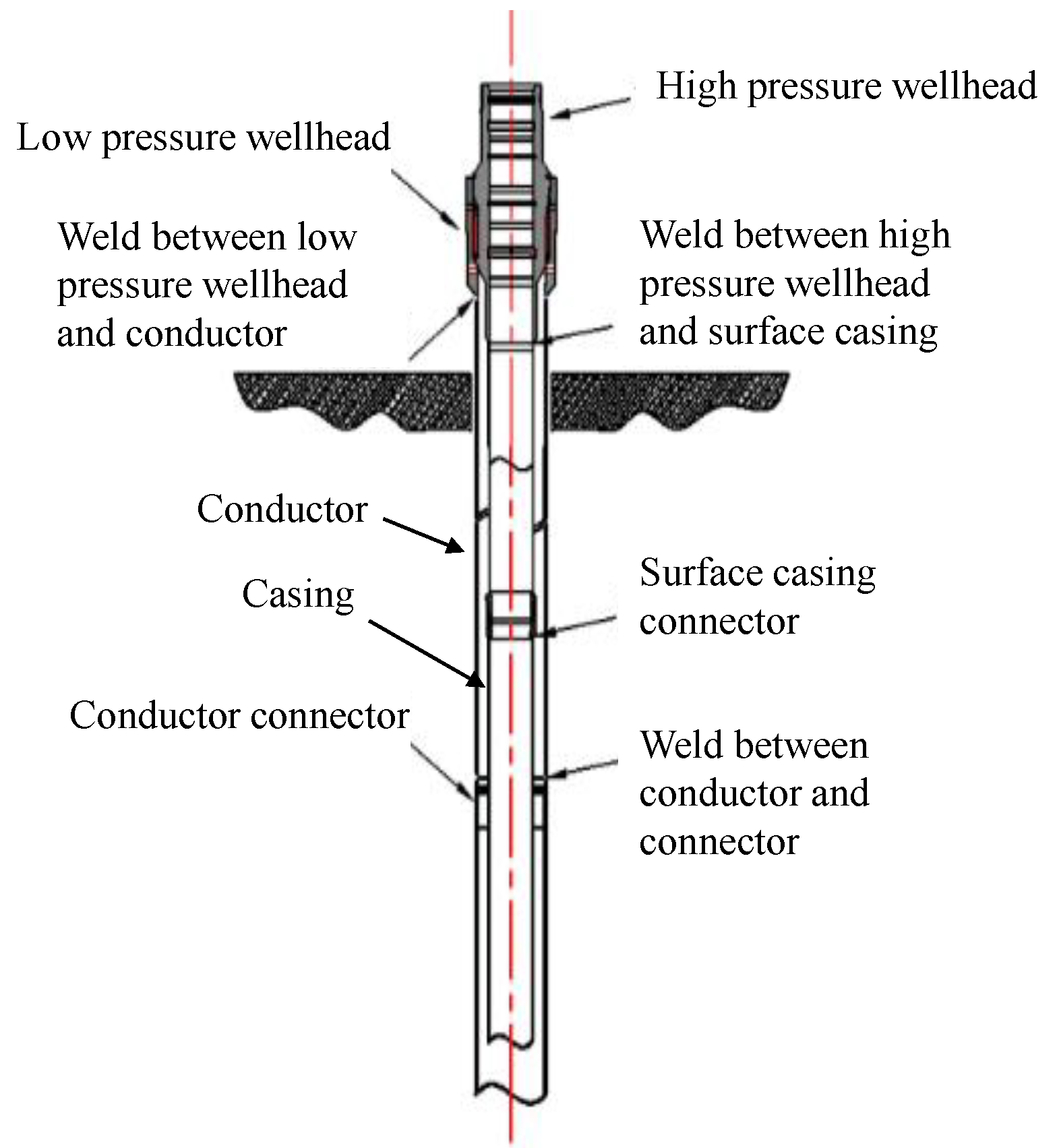
Subsea wellhead (SW) is the crucial drilling, production and well control equipment in deepwater oil and gas development. The SW system in a typical riser system (Figure 1) mainly consists of a high-pressure wellhead (HW), low-pressure wellhead (LW), conductors and casing, as shown in Figure 2. When the risers and BOPs are connected, the SW is subjected to the cyclic bending moment load caused by the movement of the drilling rig and the vibration of the risers, resulting in fatigue damage of the SW [1]. Once the fatigue resistance limit of SW is reached, the fatigue failure of SW would be induced [2]. An exploration well being drilled in the North Sea, west of Shetland, had to be abandoned 29 days after running the high-pressure housing due to the fatigue failure of the weld between the casing extension and the SW body [3]. Furthermore, many aged subsea wells in deepwater approaching the design life of 20 or more years have been reworked to enable production for many years before permanent abandonment [4]. Consequently, accumulated fatigue damage in the SW will lead to a significant increase in the fatigue failure probability.
In recent years, the growing number of researchers have shown an increased interest in the fatigue damage and the fatigue failure of SW. Greene and Grytøyr et al. [5,6] presented that the size and weight of BOP were the main factors for the fatigue damage of SW. Sunday et al. [7] revised the initial evaluation model of the SW by incorporating monitoring data. Ruschel et al. [8] proposed the univariate dimension reduction method to compute the fatigue damage of a wellhead structure considering the effect of wave type. Chang et al. [9] developed a semi-decoupled model of SW to analyze fatigue damage of SW. Li et al. [10] proposed a local stress–strain approach to assess fatigue damage of SW. Neill et al. [11] proposed an approach based on measured data to assess the SW fatigue, and the analysis results demonstrated that wave activity was one of the major factors causing the fatigue damage of SW. Chang et al. [4] presented an approach for the risk analysis of SW system fatigue failure based on Dynamic Bayesian Networks. Hørte et al. [12] estimated the fatigue reliability of SW by the Monte-Carlo and FORM/SORM method. Jaculli et al. [13] utilized stochastic analysis to estimate wellhead reliability. Whereas, the current research mainly focuses on the evaluation method of SW fatigue damage and fatigue failure analysis of SW during service life. Few researchers have studied the probability distribution characteristic of SW fatigue damage, which would be utilized to determine the relationship between the risk of fatigue failure and accumulation fatigue damage of SW conveniently and effectively.
Currently, as a reliability estimation method, the probability density function (PDF) has been widely used in many fields, such as steel bridge, nuclear power, and oil and gas equipment. Zhou et al. [14] proposed the probability the density evolution method to study stochastic seismic response and stability reliability of a vertical retaining wall in front of the pumping station pool of a nuclear power plant. Kwon et al. [15] focused on fatigue reliability assessment of steel bridges by using probability density functions of equivalent stress range based on field monitoring data. Chen [16] studied the probabilistic characteristics of the extreme loads to propose the global time-dependent reliability analysis model of ageing platforms. Miao and Liu et al. [17,18] presented the seismic functional reliability assessment approach and a lifecycle operational reliability assessment framework for water distribution networks based on the probability density evolution method. Xian et al. [19] proposed probability density evolution and the explicit time-domain combination method to analyze the system reliability of energy-dissipation structures. Feng et al. [20] presented the reliability approach based on probability density to quantify the structural robustness of reinforced concrete structures subjected to progressive collapse. Gao et al. [21] presented a novel nonlinear time-varying fatigue reliability analysis method to improve the accuracy and efficiency of time-varying reliability analysis. However, at present, research on the fatigue failure of SW by a probability method is found sporadically in related literature.
Generally, it is necessary to calculate a heap of data for acquiring the PDF. It is difficult to compute enough fatigue damage data of SW by the finite element analysis (FEA) method due to the complicated and time-consuming calculation process. Recently, artificial neural network (ANN) development has been widely used to generate a huge amount of data due to its robustness and adequate nonlinearity and excellent universal approximation capability for continuous bounded functions [22,23,24], whereas a conventional ANN algorithm may encounter the overfitting problem, i.e., lower bias but larger variance. As the Bayesian Regularization Artificial Neuron Network (BRANN) is a robust and accurate function approximation algorithm that adopts the Bayer’s theory causing its superior performance, the BRANN has better generalization capacity especially for a limited data set [25,26,27], which could be used to develop a robust data-driven model to generate huge amounts of data quickly [28,29].
The objective of the present work is to propose a BRANN-based probability methodology for predicting the fatigue failure probability of SW. The BRANN is applied to develop a BRANN fatigue damage (BRANN-FD) model using the limited fatigue damage data acquired by a traditional fatigue analysis method. Based on the developed BRANN-FD model, a large amount of fatigue damage data is generated with less time consuming. Subsequently, the PDF of SW fatigue damage is assessed by the parametric and non-parametric estimation methods to obtain the possible fatigue damage of SW in each operation and the accumulation fatigue damage of SW during service life. By logistic regression, the nonlinear relationship between the fatigue failure probability and accumulation fatigue damage could be determined.
The rest of this paper is organized as follows. Section 2 introduces the background of the BRANN, the parametric and non-parametric estimation methods, as well as the logistic regression. In Section 3, the BRANN-based probability methodology is proposed for predicting the fatigue failure probability of SW. Section 4 provides a case study regarding the application of a proposed BRANN-based probability prediction method of SW fatigue failure. Finally, the research conclusions are summarized in Section 5.

2. Background

2.1. BRANN

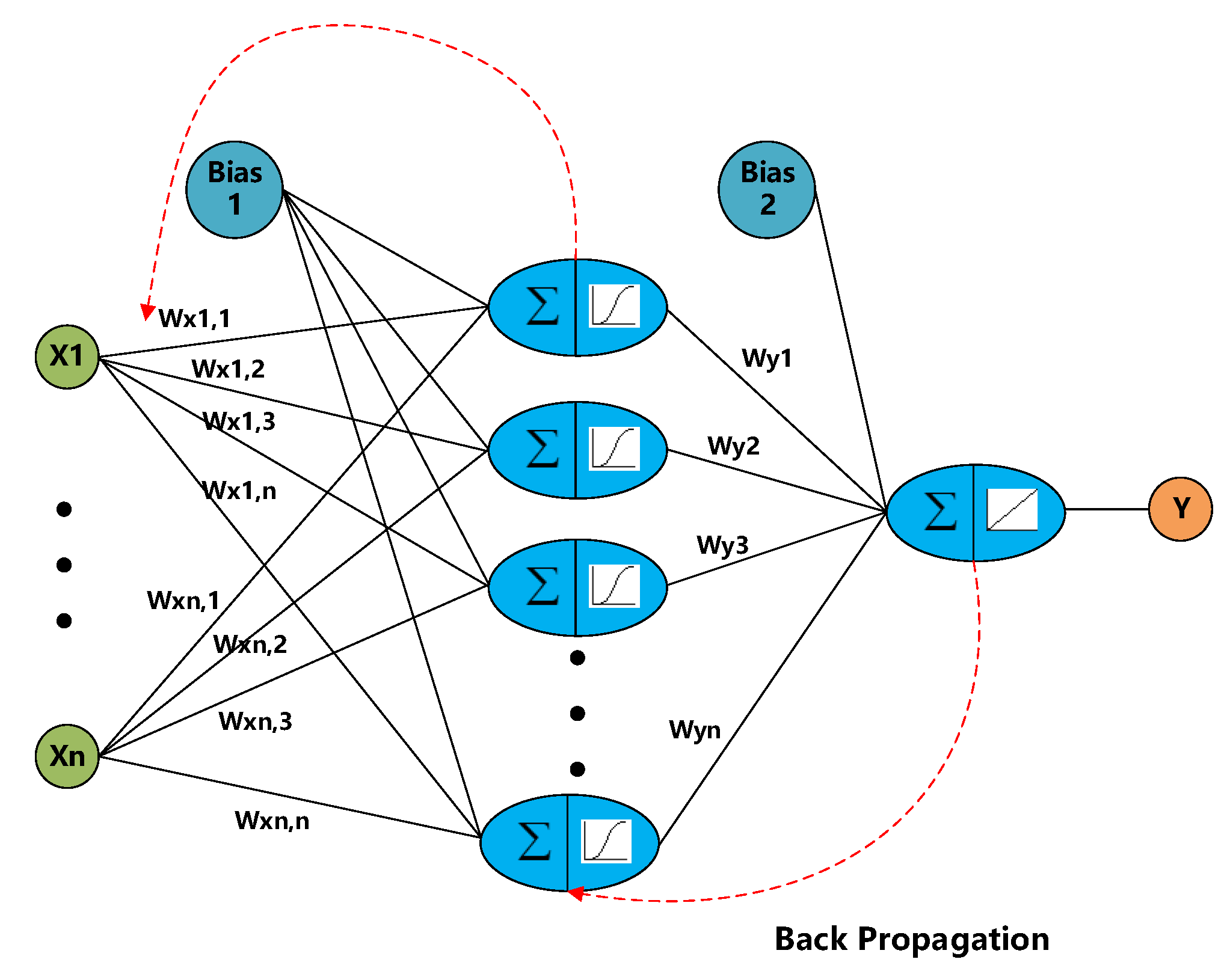
The BRANN-based model is developed according to the multi-layer perception (MLP) with the back-propagation (BP) algorithm (Figure 3), but it overcomes the overfitting problem of the conventional BP algorithm, i.e., lower bias but larger variance. As an alternative, BRANN has better generalization capacity and robustly determines the complex nonlinear relationship between the input and output data.
The BRANN minimizes the objective function F including a combination of mean squared error function E D and the weight attenuation function E W , and determines the optimal weights and objective function parameters α , β with a probability manner [24,30]. Consequently, BRANN can efficiently reduce those parameters that have less contributions to reduce the error function [31]. The objective function for the BRANN is shown as follows:
F = β E D + α E W
E D = 1 N i N ( y i t i ) 2 = 1 N i N e i 2
E W = 1 2 i m w i 2
where α and β present hyper-parameters, which are used to control the distribution of other parameters; w is the weights; m is the number of those weights; D = ( x i , t i ) means the data of training set with i = 1, 2, …, N, where N is the total number of the training sets (input–output pairs); y i means the i th output value corresponding to the i th training set (input–output pair).
In the BRANN, the initial weights are randomly set. With these initial weights, the density function for the weights can be updated according to Bayer’s rule:
P ( w | D , α , β , M ) = P ( D | w , β , M ) P ( w | α , M ) P ( D | α , β , M )
where M is the particular neural network architecture adopted; P ( w | α , M ) is the prior density, which represents our knowledge of the weights before any data are collected; P ( D | w , β , M ) is the likelihood function, which is the probability of the data occurring, given the weights w ; P ( D | α , β , M ) is a normalization factor, which is given in Equation (5).
P ( D | α , β , M ) = + P ( D | α , β , M ) P ( w | α , M ) d w
If Gaussian distribution is assumed to the noise of training set data and weights, the probability densities can be calculated by:
P ( D | w , β , M ) = 1 Z D ( β ) exp ( β E D ) = ( π / β ) N / 2 exp ( β E D )
P ( w | α , M ) = 1 Z W ( α ) exp ( β E W ) = ( π / α ) m / 2 exp ( β E W )
If these probability densities are substituted into Equation (4), the probability equation becomes:
P ( w | D , α , β , M ) = 1 Z W ( α ) 1 Z D ( β ) exp ( ( β E D + β E W ) ) P ( D | α , β , M ) = 1 Z F ( α , β ) e x p ( - F ( w ) )
In the BRANN, determining the optimal weights means maximizing the posterior probability P ( w | D , α , β , M ) , which is equivalent to minimizing the regularized objective function F [24]. The Levenberg–Marquardt (LM) algorithm is a simple and accurate alternative for function approximation, which iteratively updates the weights as follows [32]:
w k + 1 = w k [ H + μ I ] 1 J t r e
where e = ( e 1 , e 2 , ... , e N ) is the error vector containing the output errors for each input vector used on training the network. k is the iteration number and μ is the damping parameter, which is summed to every number of the approximate Hessian diagonal before the system is solved for the gradient. H is the Hessian matrix, which can be expressed by H = J t r J , where J is the Jacobian matrix, which can be calculated as follows:
J = [ e 1 ( x 1 , w ) w 1 e 1 ( x 1 , w ) w m e N ( x N , w ) w 1 e N ( x N , w ) m ]
After the optimal weights under the maximum posterior probability w M P are determined, the optimal values for α M P and β M P can be determined as follows:
η = w M P ( α M P × t r ( H M P 1 ) )
β M P = ( N η ) / ( 2 × E D ( w M P ) )
α M P = η / ( 2 × E W ( w M P ) )
where M P means the maximum posterior; η is a measure of how many parameters in the neural network are effectively used in reducing the error function.

2.2. Parametric and Non-Parametric Estimation

For the parametric estimation, the prior knowledge of data distribution needs to be known, and then, the Maximum Likelihood Estimation (MLE) can be employed to estimate those related unknown parameters of assumption distribution. As the SW is a structural component, the fatigue damage of SW is deemed to follow the Weibull distribution or the Lognormal distribution. In contrast, with respect to the non-parametric estimation, only the sample data are used to estimate the distribution characteristic of data.

2.2.1. Weibull Distribution

The Weibull distribution has been used to fit many stress spectra for marine structures subjected to wave load in the offshore oil and gas industry [33]. Additionally, the two-parameter Weibull distribution, whose PDF is given in Equation (14), has been extensively used over the past decades for fitting data [34,35].
f ( x ) = k λ ( x λ ) k 1 exp [ ( x λ ) k ] , x 0
where x is the variable; k and λ are the shape and scale parameters, respectively. Furthermore, the related mean μ and standard deviation σ are shown in Equations (15) and (16).
μ = λ Γ ( 1 + 1 k )
σ = λ [ Γ ( 1 + 2 k ) Γ 2 ( 1 + 1 k ) ]
where Γ is the Gamma function. When the variable is assumed as t, it can be expressed as follows:
Γ ( t ) = 0 + x t 1 exp ( x ) d x

2.2.2. Lognormal Distribution

The Lognormal distribution is established based on the normal distribution. For the random variable X′, if Y′ = ln X′ is normal distribution, and the mean and the standard deviation are the μ and σ, respectively. Then, the random variable X′ obeys the Lognormal distribution of μ and σ2. The PDF of Lognormal distribution is shown in Equation (18).
f ( x ) = { 1 σ x 2 π exp ( ( ln x μ ) 2 2 σ 2 ) , x > 0 0 , x 0

2.2.3. Kernel Density Estimation

Kernel density estimation (KDE) proposed by Rosenblatt and Parzen is used to estimate the PDF for the unknown density function in the probability theory, which is one of the non-parametric test methods. Since the KDE approach studies the distribution characteristics of data from the data sample itself without assuming data distribution, it is paid significant attention to statistical theory and application field. The fixed-width kernel sampling density is given, as follows:
k ( x ) = 1 N i = 1 N 1 h n K ( x x i h )
where xi, i = 1, 2, …, N are samples used for constructing the PDF k(x); n is the dimension of inputs, h is the bandwidth, and K is the kernel PDF.
A range of kernel functions is commonly used: uniform, triangular, biweight, triweight, Epanechnikov, normal, and others [36]. Due to its convenient mathematical properties, the normal kernel is a popular choice, and it is also used in this work, which means K(x) = φ(x), where φ is the standard normal PDF. Note that for the PDF of fatigue damage of SW, only a one-dimensional kernel sampling density is needed.

2.3. Logistic Regression

Considering a Bernoulli experiment with a binary output variable as Y(0,1), the binomial logistic regression can be used to predict the outcome of the experiment using a probability function P ( x ) = P ( Y = 1 | X = x ) where X can be a set of parameters (covariates). Having the logistic transformation (or logit) of P ( x ) as a linear function of x as ln P ( x ) 1 - P ( x ) = β 0 + β 1 x , the probability function can be presented in Equation (20):
P ( x ) = e ψ ( x ) 1 + e ψ ( x )
where ψ ( x ) = β 0 + β 1 x is the logit function, and β0 and β1 are the parameters of the logistic regression, which can be estimated by maximizing the likelihood function of P ( x ) given an observation of the experiment outcome, as shown by Hosmer and Van [37,38] using a Bayesian inference scheme. Assuming a Bernoulli experiment (Y = 1 if the fatigue failure of SW and Y = 0 if the SW survives) with a probability distribution of P ( x ) , the likelihood function for n observations can be developed as Equation (21):
L i k e l i h o o d = i = 1 n P ( Y = y i | X = x i ) = i = 1 n P ( x i ) y i ( 1 P ( x i ) ) 1 y i

3. Methodology of Establishing the Probability Density Function of Fatigue Damage of SW

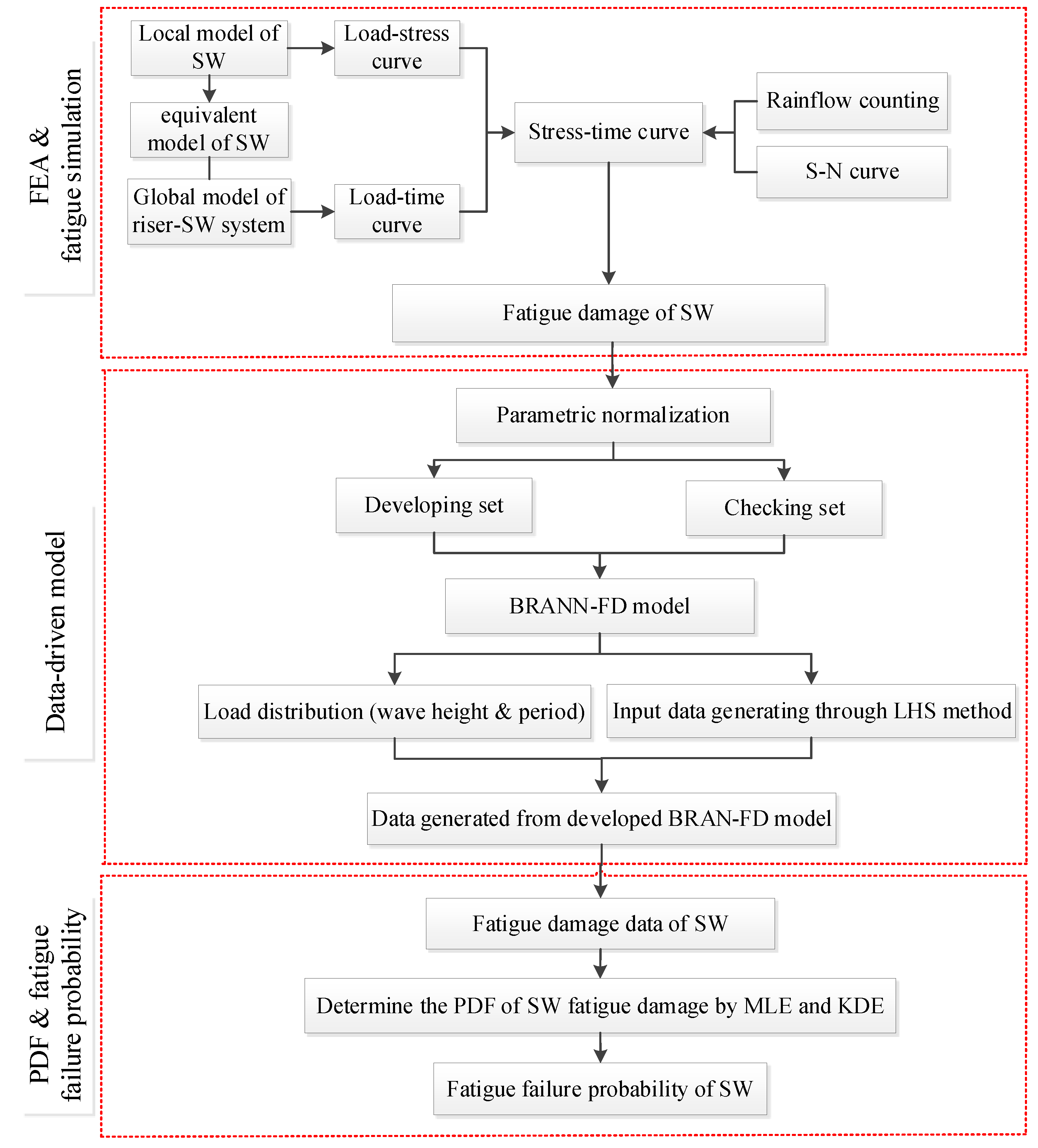
Figure 4 presents the schematic of proposed methodology, which includes three parts: FEA and fatigue damage simulation [39,40], data-driven model, as well as the establishing PDF of fatigue damage and predicting probability of fatigue failure for SW. Each part is addressed as follows:
Step 1: Local analysis. Local analysis of the SW system is applied to build the load–stress curve and the equivalent model of the SW. Then, the equivalent model is put into the global model forming the semi-decoupled model. The detailed modeling process of equivalent model is shown in references [9,41,42] for more detail.
Step 2: Fatigue damage analysis. Global analysis of the semi-decoupled model is employed to extract cyclic fatigue dynamic load of SW under the different wave loads, and then, the stress–time curve can be determined. After the stress range is obtained by the rainflow counting, the fatigue damage of SW is calculated by the S−N curve and Palmgren-Miner’s rule.
Step 3: Developing and checking the BRANN-FD model. After the simulation data are divided into developing set and checking set, the BRANN is used to train the BRANN-FD model under the different number of hidden neurons. Simultaneously, the coefficient determination R 2 between estimated results and simulation results of the developing set is calculated as well as R 2 between the estimated results and simulation results of the checking set. Both R 2 of the developing set and checking set are all viewed as the indicator to establish the appropriate BRANN-FD model. For the development process of the BRANN model, the interested readers may see references [25,28,43] for more detail.
Step 4: Input loads data. Generally, it is assumed that the significant wave height follows a Weibull distribution with two parameters, and the wave period follows Lognormal distribution. Based on the environment loads data in the South China Sea, the Maximum Likelihood Estimation (MLE) is applied to estimate those unknown parameters in the above distributions. A variety of input parameters are generated through the Latin Hypercube Sampling (LHS) method based on the distributions of the height and period of the wave.
Step 5: The thousands of numbers of fatigue damage data generated. Based on the developed BRANN-FD model and the obtained input loads data, a huge amount of fatigue damage data of SW are generated accurately and efficiently.
Step 6: PDF of fatigue damage assessed. The parametric and non-parametric estimation methods are applied to build the PDF of fatigue damage for SW based on the thousands of numbers of fatigue damage data. By comparison, the reasonable probability distribution characteristic of fatigue damage is determined.
Step 7: Fatigue failure probability predicted. The possible fatigue damage in each operation and the accumulation fatigue damage of SW during service could be easily calculated by PDF. Then, the fatigue failure probability of SW would be predicted by logistic regression.

4. Case Study

4.1. Fatigue Damage Analysis of SW

4.1.1. Basic Data

The SW of SS10 (Table 1) was taken as an example to calculate the fatigue damage in the drilling operation. The water depth of the target well was about 650 m in the South China Sea, and the drilling riser configuration is listed in Table 2. The one-year return period current profile and the wave load in the South China Sea were selected. Furthermore, the joint probability of occurrences of significant wave height H s and wave period T p described by a scatter diagram was adopted, as shown in Table 3. The wave load was the primary factor causing the fatigue damage of SW, while the current had little contribution [11]. Consequently, the wave load could be viewed as variable, and the current load could be considered constant. In this study, the fatigue damage of the WH weld and LH weld were selected to investigate the PDF of SW fatigue damage, as they have been regarded as the most critical fatigue position in the SW system.

4.1.2. Fatigue Damage Calculation Based on Semi-Decoupled Model

In the local model of the SW system, the HW, LW, conductor, surface casing and the cement between the conductor and surface casing were the significant structures to be subjected to the fatigue dynamic loads; thus, they were modeled by a solid element to ensure analysis accuracy [10,44,45]. The beam element was used to model the other region improving the calculation speed. Due to the complex structure of the SW system, including the contact, the hexahedral structured mesh was used, and the size of the mesh was determined by mesh sensitivity analysis. In addition, in order to improve the analysis accuracy, the mesh of the contact and stress concentration region was further subdivided. Furthermore, the soil resistance was represented by non-linear springs to ensure the accuracy of the interaction between the soil and conductor as well as calculation speed. The lower boundary of the local model was supposed to be extended to at least 50 m below the mud line to avoid the influence of the fixed restraint of the bottom, and the upper boundary of the local model should be at the lower flex joint [46]. Then, the local model of the SW system was established.
By local analysis, the load–stress curve and the parameters of the equivalent model were determined as shown in Figure 5 and Table 4, respectively. As the SW system is the complicated structure, the calculation of the local model for SW would be time consuming.
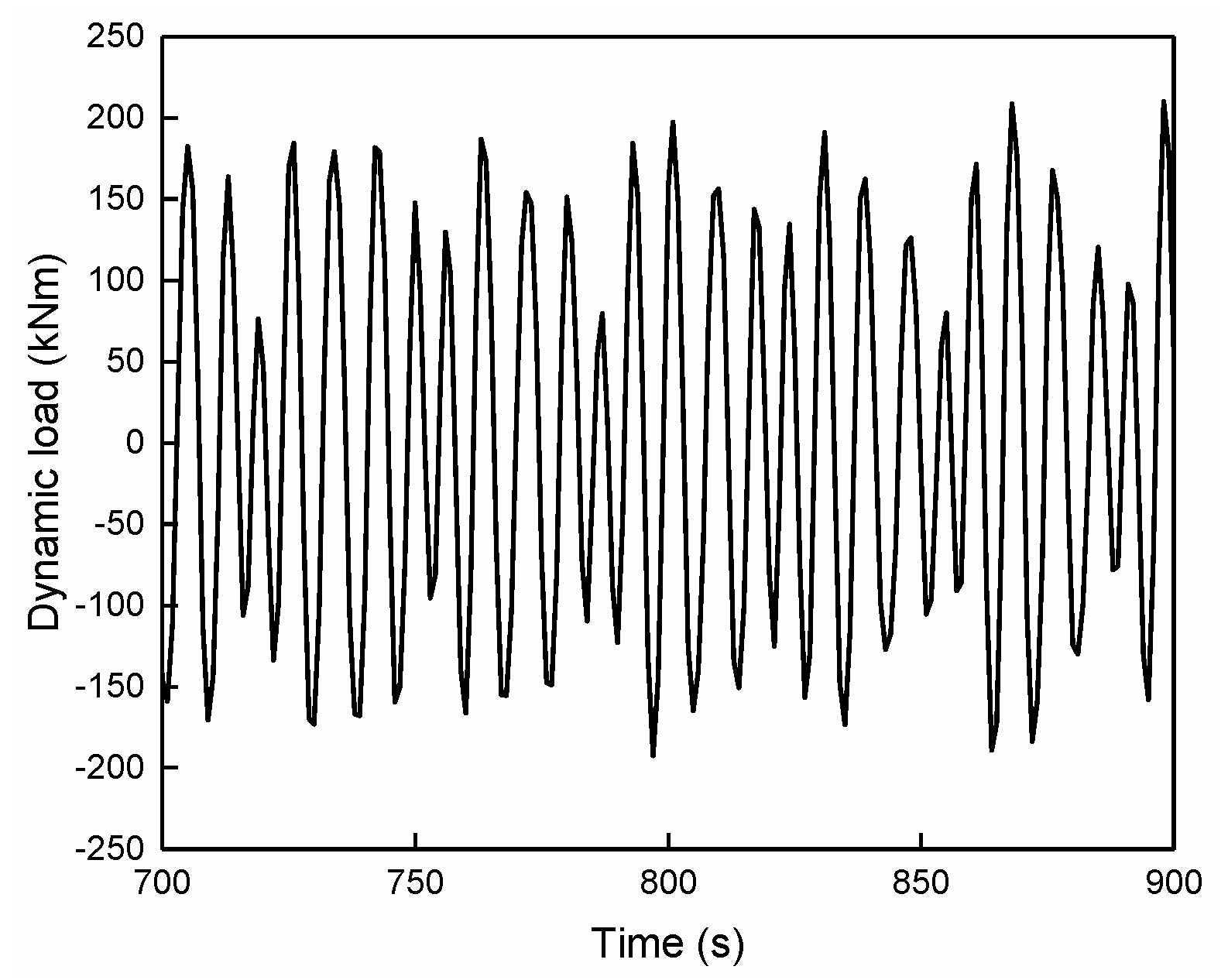
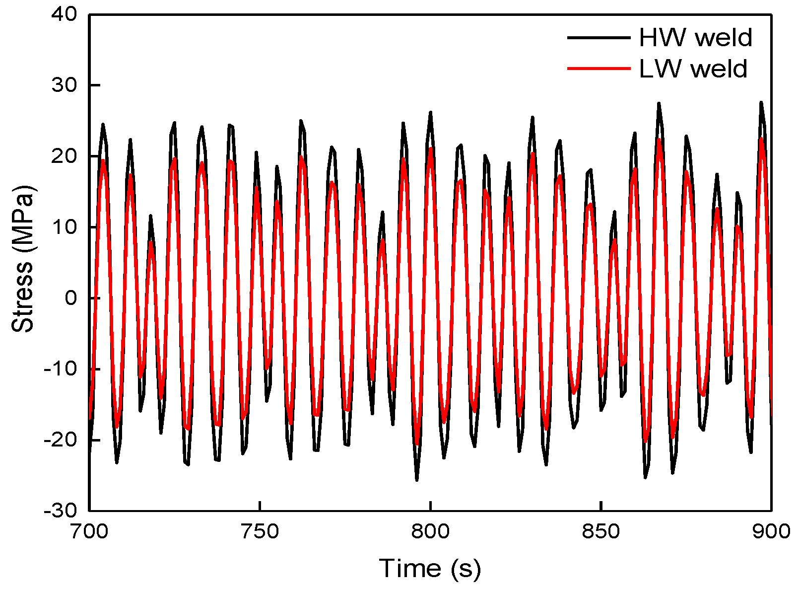
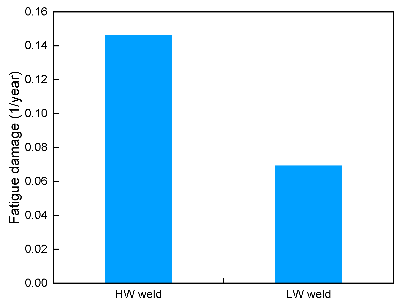
The equivalent beam model of the SW system was put into the riser−BOPs−wellhead model to build the semi-decoupled model. The semi-decoupled model was employed to obtain the load−time curve of SW in drilling operation by dynamic analysis. Figure 6 shows the load−time curve of SW under the wave load of HS = 3.25 m and TP = 9.5 s from 700 to 900 s. After the curves of stress response of the HW and LW welds were calculated, as shown in Figure 7, the stress ranges of the HW and LW welds were obtained by the rainflow counting. Subsequently, the fatigue damage of SW was calculated by the S−N curve and Palmgren−Miner’s rule as given in Figure 8. It was considerably time consuming to conduct fatigue damage analysis of SW for only one wave load condition, as the dynamic analysis time of 3000 s was adopted to obtain a realistic and stable dynamic response of the riser system.

4.2. BRANN Fatigue Damage Model

In terms of the wave scatter diagram, 127 wave loads were selected to compute fatigue damage of the HW and LH welds. Generally, the simulations number of the developing set employed could influence model generalization significantly, as the accuracy and robustness of the developed model could be improved with the increment number of simulations. Furthermore, the simulation number of checking sets should be larger than those of developing sets to ensure the effectiveness of checking. However, a large number of simulation inputs would bring great computational burden for engineering application. Accordingly, it was necessary to balance the trade-off between the robustness and the inputs. Eventually, according to the limited 127 simulation results, the developing set had 60 simulations and the checking set had 67 simulations for BRANN-FD model development. Additionally, the number of hidden neurons that was difficult to determine was analyzed from 1 to 20 to obtain the optimal value.
Figure 9 demonstrates the robustness analysis of the BRANN-FD models for HW and LW welds under varied hidden neuron numbers. The BRANN-FD models of the HW and LW welds could show the coefficient determination R 2 results of the developing set and checking set under different hidden neuron numbers. As can be seen in Figure 9a, the coefficient determination R 2 of the developing set becomes steady and approaches 1 with the increase in neural number. Meanwhile, the R 2 of the checking set also becomes stable and comes close to 0.978 with the increment in the neural number. When the neural number is 10, the R2 of the checking set reaches the maximum, 0.978. Thus, the determined optimal number of hidden neurons is 10. The analysis results illustrate that the developed BRANN-FD model of the HW weld had no overfitting problem, and the BRANN-based model was quite robust and accurate. Similarly, for the BRANN-FD model of the LW weld, the same results would also be obtained.

4.3. Probability Density Function of Fatigue Damage

4.3.1. PDF of Fatigue Damage Determined by Parametric Estimation

Generally, the significant wave height is assumed to follow the two-parameter Weibull distribution whose PDF is shown in Equation (14). Correspondingly, the wave period T P conditional on H s is practically modeled by a Lognormal distribution whose PDF is shown in Equation (18). The MLE was carried out to estimate those unknown parameters based on the wave scatter diagram listed in Table 3, and the evaluation results are given in Table 5. According to the distributions of wave height and period, the LHS method was performed to generate 10,000 sets of reasonable random input data. Then, applying the developed BRANN-FD models and input data, the 10,000 sets of fatigue damage data of the HW and LW welds were generated fast, respectively. The huge amounts of fatigue damage data were used to assess the PDF curves of fatigue damage of the HW and LW welds, respectively.
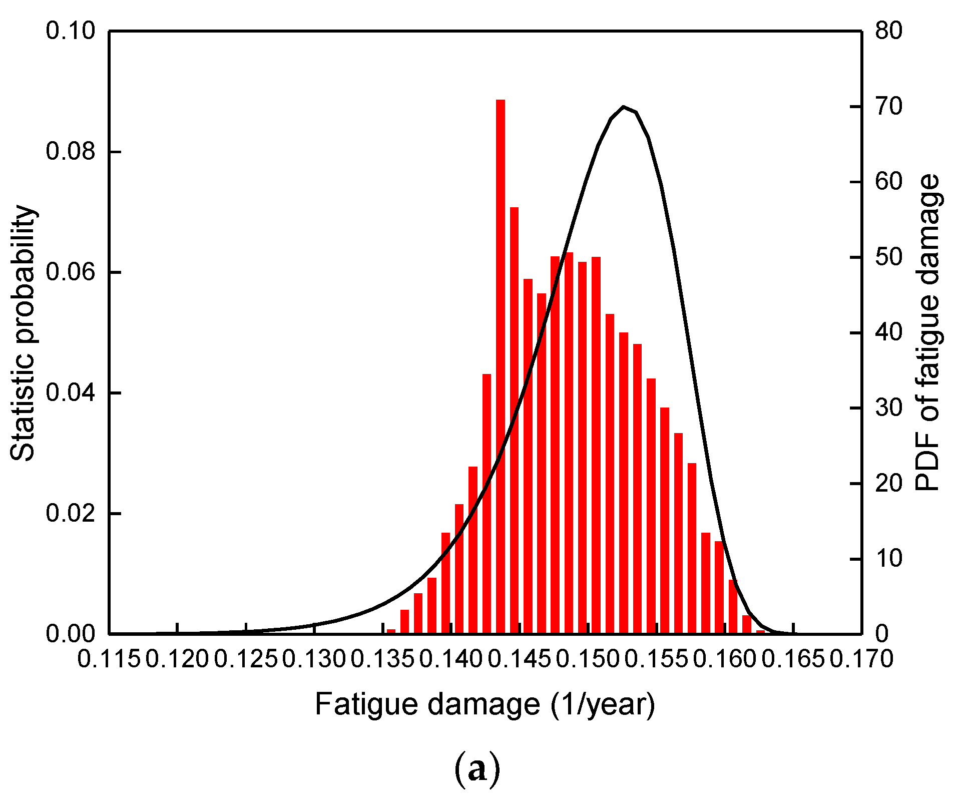
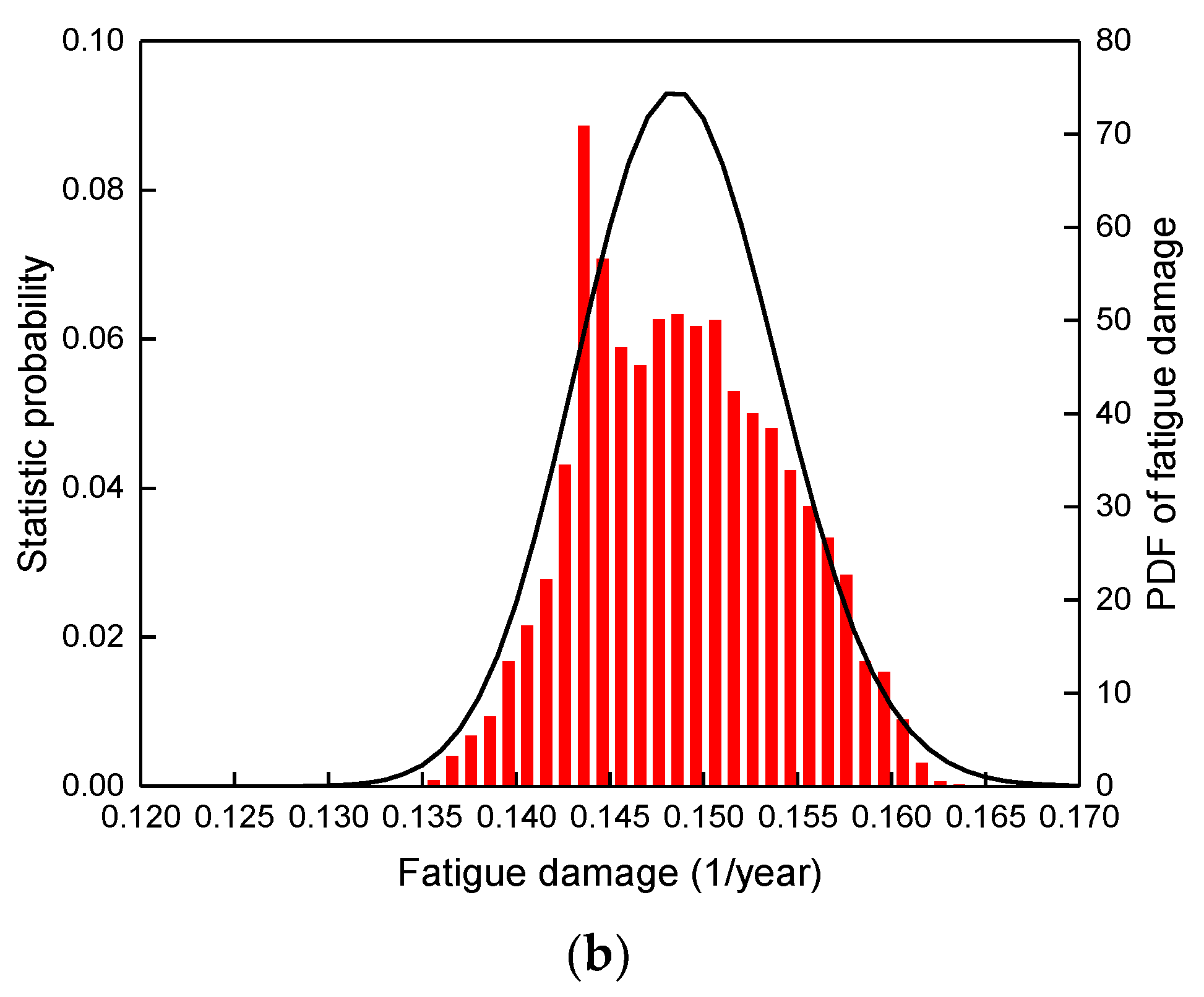
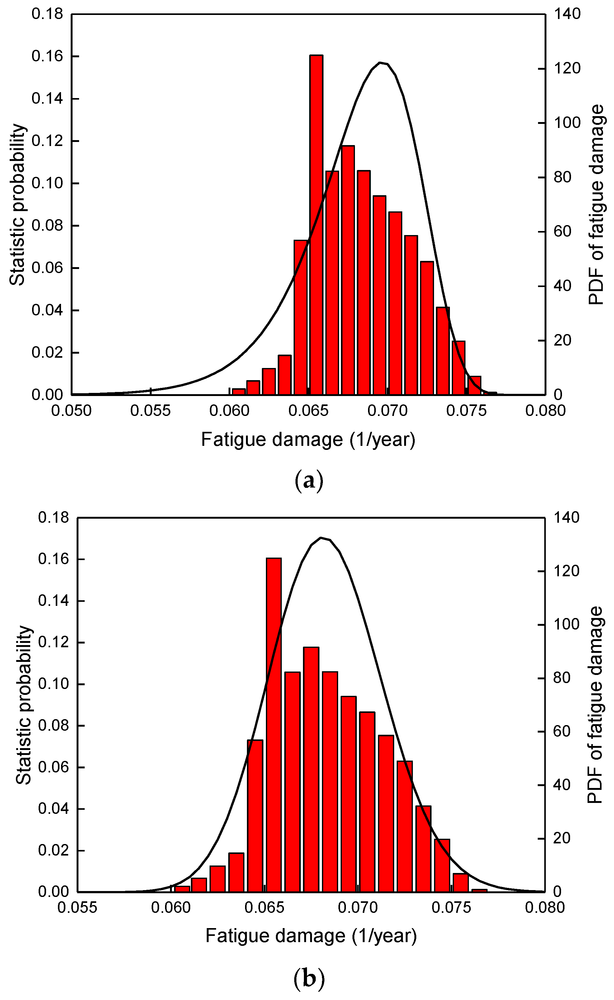
In parametric estimation, it was assumed that the fatigue damage of SW followed the Weibull distribution or the Lognormal distribution. Based on the fatigue damage data, the unknown parameters were estimated by the MLE method. For the HW weld, the estimated PDF curves of fatigue damage are shown in Figure 10. Simultaneously, the 10,000 sample data were divided into different stages in the same interval, 0.001, and the occurrence probability of fatigue damage (OPFD) for different stages was calculated as given in Figure 10. As the PDF of fatigue damage presents the occurrence possibility for a certain fatigue damage, the statistic OPFD of different stages would be regarded as a criterion to acquire the most possible probability distribution characteristic of fatigue damage of the HW weld. Similarly, the statistic OPFD of different stages and the PDF curves of fatigue damage for the LW weld were obtained as shown in Figure 11.
As can be seen from Figure 10, for the statistic OPFD, when the fatigue damage of the HW weld is less than 0.147 a−1, the statistic OPFD of different stages increases first and then decreases with the increment in fatigue damage, while the same regulation also occurs when fatigue damage of the WH weld is between 0.147 and 0.165 a−1. This means that the peak value of PDF should be in the range of 0.144 and 0.151 a−1, and the PDF curve of fatigue damage should have the same change tendency and speed with the statistic OPFD.
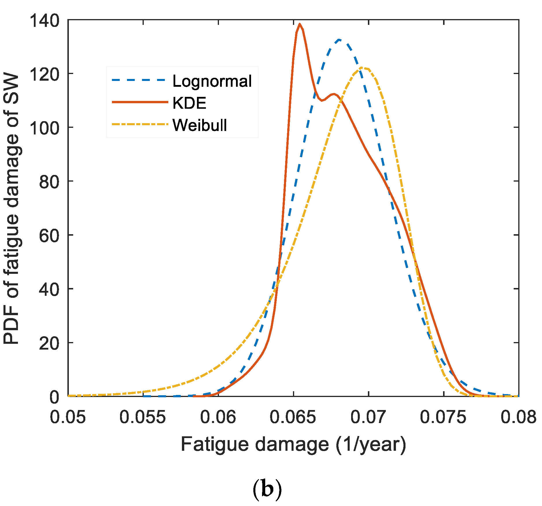
In Figure 10a, the peak value of the PDF curve is between 0.152 and 0.154 a−1, and the change speed and tendency of the PDF curve is different from that of the statistic OPFD. With respect to the Lognormal distribution (Figure 10b), the peak value of the PDF curve is between 0.148 and 0.150 a−1, and the change speed and tendency of the PDF curve is closer to that of the statistic OPFD. Similarly, Figure 11 also demonstrates that the change speed and tendency of the PDF curve estimated by Lognormal distribution is almost in agreement with that of the statistical OPFD. By comparison, the results illustrated that the Lognormal distribution was more appropriate to represent the probability distribution characteristic of SW fatigue damage rather than the Weibull distribution.

4.3.2. PDF of Fatigue Damage Determined by Non-Parametric Estimation

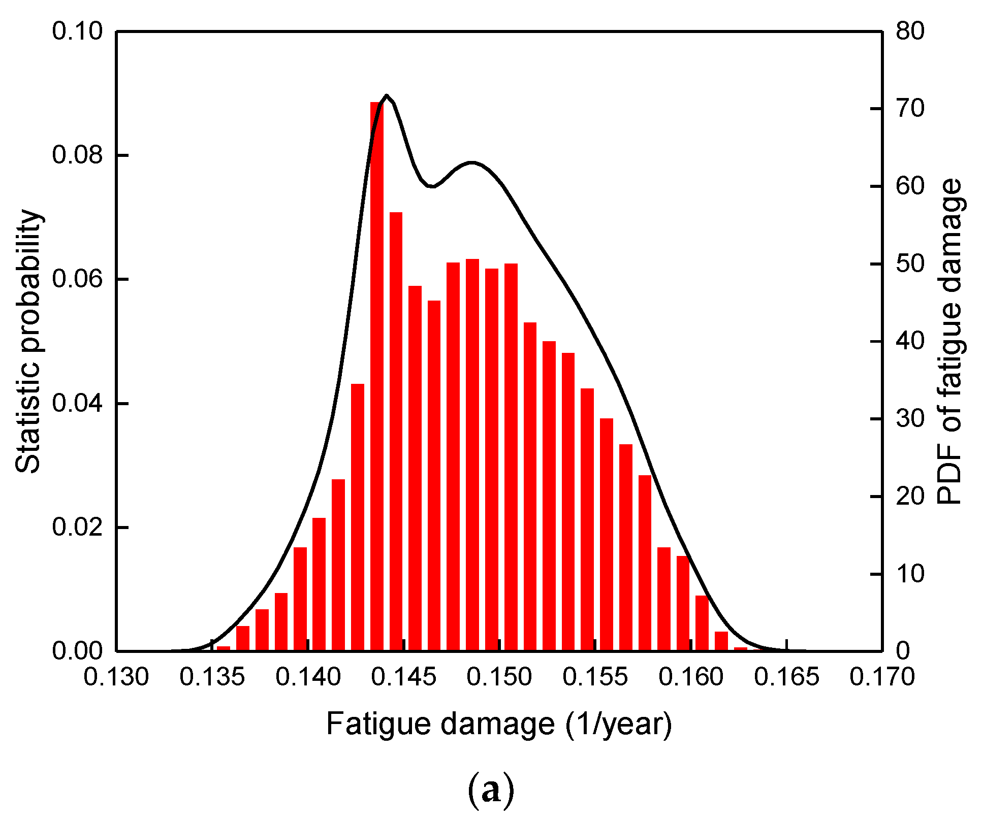
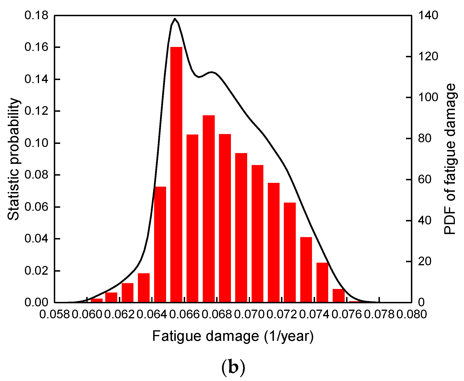
Different from parametric estimation, prior knowledge of data distribution is not needed for the non-parametric estimation. Thus, the KED with an appropriate kernel bandwidth is employed to obtain the distribution characteristic of fatigue damage for SW without prior knowledge of fatigue data distribution, as shown in Figure 12. As seen from Figure 12, for the HW weld, the peak range of the estimated PDF curve as well as the change speed and tendency of the PDF curve are in agreement with that of the statistical OPFD. Furthermore, the same results could be obtained by analysis of the LW weld. The results showed that the non-parametric estimation was more appropriate to be used to determine the PDF of fatigue damage of SW, as a distribution characteristic of SW fatigue damage data was not assumed.
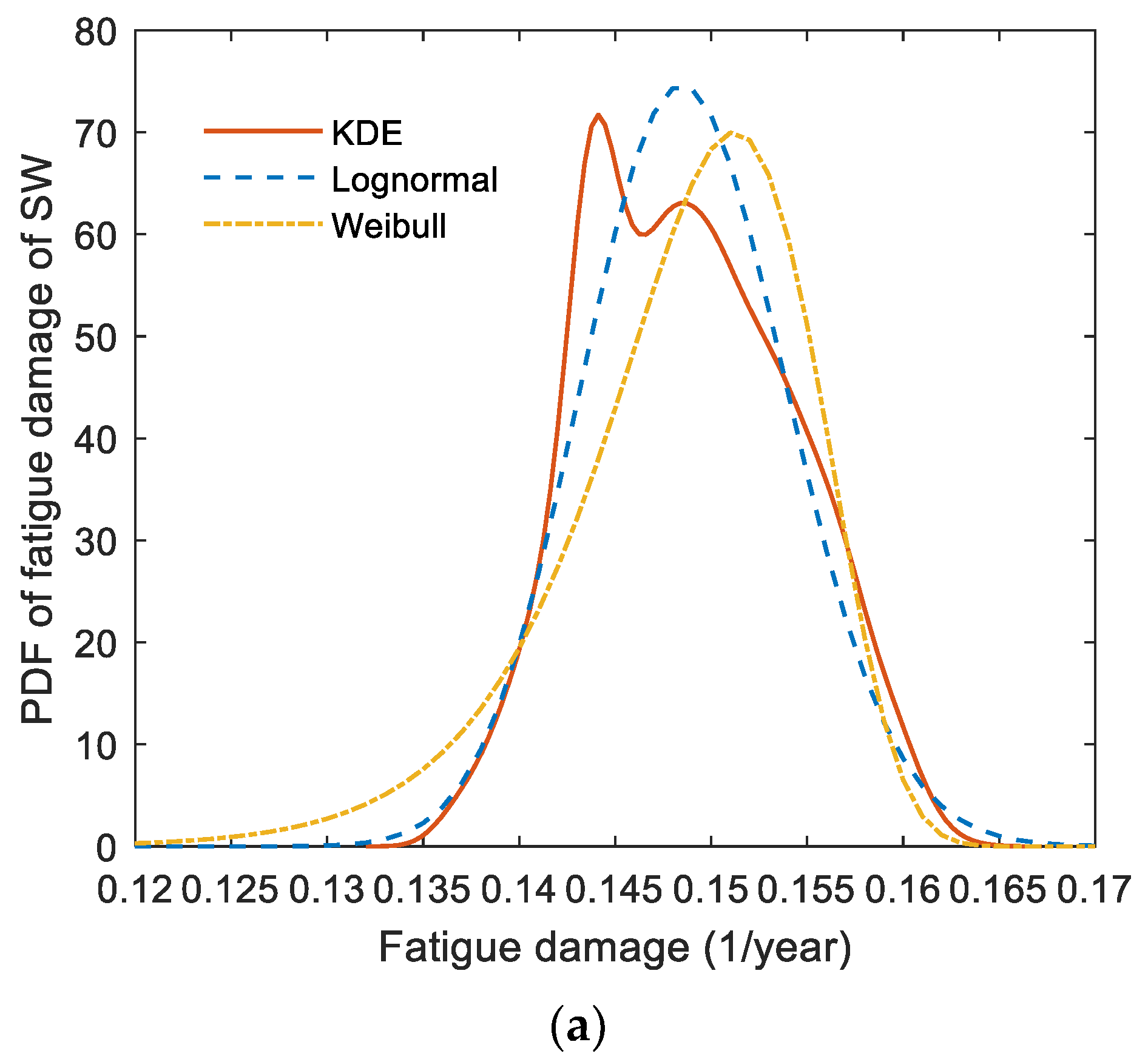
However, the PDF of fatigue damage obtained by non-parametric estimation was not the common distribution form; thus, it was difficult to be used to calculate the fatigue damage and accumulation of fatigue damage. Therefore, the most appropriate common distribution form of fatigue damage was supposed to be determined by the comparison of parametric and non-parametric estimation results. In Figure 13, the comparison results show that the PDF estimated by KDE is basically similar to the Lognormal distribution rather than to Weibull distribution. The results demonstrated that the PDF of SW fatigue damage would be considered as the approximate Lognormal distribution. Based on the distribution characteristics of SW fatigue damage, the possible fatigue damage of SW in each operation could be obtained by the LHS method quickly and conveniently, and the randomness of the fatigue damage could also be taken into consideration. Thus, the accumulation fatigue damage of SW could be calculated rapidly.

4.4. Fatigue Failure Probability of SW

The fatigue damage of the HW weld was larger than that of the LW weld, which could represent the fatigue damage of SW to predict the fatigue failure probability of SW. As the PDF of fatigue damage followed Lognormal distribution, the unknown parameters of PDF could be assessed for drilling and completion and workover operation, as listed in Table 6. Considering the operation sequence of SW during service life, the fatigue damage data of SW in each operation were generated by LHS and relevant PDF, and the accumulation fatigue damage of SW was calculated. Once the accumulation fatigue damage of SW was more than 1, the accumulation calculation was stopped.
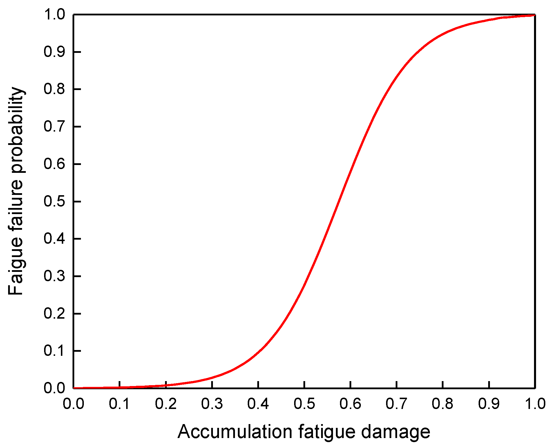
When the accumulation fatigue damage of SW during service life was more than 1, it was considered as failed. By the MLE, the optimal values of the logistic regression parameters were calculated, which were β 0 = −7.3868 and β 1 = 12.8476. Furthermore, the relationship between accumulation fatigue damage and the fatigue failure probability was determined as shown in Figure 14. It can be seen in Figure 14 that during the entire life of SW, the fatigue failure probability nonlinearly increases with the increment of the accumulation fatigue damage. When the fatigue damage is less than 0.3, the fatigue failure probability is very low, whereas when the fatigue damage is between 0.3 and 0.7, the possibility of fatigue failure increases quickly. Once the accumulation fatigue is more than 0.7, the fatigue failure probability is close to 0.9, which means that the corresponding risk analysis is supposed to be taken to propose some preventive control measures for mitigating fatigue failure risk, especially for the aged wellhead.

5. Conclusions

This study presents a probability methodology for predicting the fatigue failure probability of SW based on BRANN. A case study demonstrates how the BRANN could be effectively manipulated to build the PDF of SW fatigue damage and to predict the fatigue failure probability of SW. The main achievements are summarized as follows.
Fatigue damage analysis of SW provides the data of developing and checking sets to train the BRANN-based model. The BRANN-FD model with 10 hidden neurons is proven to be the most efficient and robust since the R 2 of the checking set would become stable and come close to 0.978, which would be used to generate a large number of fatigue damage data of SW with negligible computational cost.
The non-parametric estimation is more appropriate to be used to acquire the probability distribution characteristic of SW fatigue damage, as probability distribution characteristic of SW fatigue damage data is not assumed. By comparison of the parametric and non-parametric estimation results, the PDF of SW fatigue damage would be deemed as the approximate Lognormal distribution, which could be applied to obtain the possible fatigue damage in each operation and accumulation fatigue damage during service life conveniently.
Based on the probability distribution characteristic of SW fatigue damage, the predicted relationship between the fatigue failure probability and accumulation fatigue damage is that the fatigue failure probability of SW nonlinearly increases with the increment in the accumulation fatigue damage. When the accumulation fatigue damage is more than 0.7, the fatigue failure probability is close to 0.9. Thus, some preventive control measures should be taken to mitigate the fatigue failure risk of SW.

Author Contributions

Conceptualization, Y.C.; Data curation, J.S.; Formal analysis, J.L. and N.Z.; Funding acquisition, Y.C.; Investigation, Q.G. and Y.D.; Methodology, J.L.; Project administration, J.L.; Resources, G.C.; Supervision, G.C.; Validation, X.L.; Writing—original draft, J.L.; Writing—review and editing, X.L. and J.L. All authors have read and agreed to the published version of the manuscript.

Funding

The authors gratefully acknowledge the financial support provided by the National Natural Science Foundation of China (no. 52071337) and the Technological Projects of CNPC under Grant (no. ZD2019-184-004).

Institutional Review Board Statement

Not applicable.

Informed Consent Statement

Not applicable.

Data Availability Statement

Not applicable.

Acknowledgments

The authors would like to thank the editors and reviewers for their many constructive suggestions and comments that helped improve the quality of the paper.

Conflicts of Interest

The authors declare no conflict of interest.

References

  1. Chen, G.; Li, J.; Chang, Y.; Wang, K.; Xiu, Z.; Liu, H.; Xu, L.; Sheng, L. Influencing factors for fatigue damage of underwater wellhead system of deepwater oil and gas. Acta Pet. Sincia 2019, 40, 141–151. [Google Scholar]
  2. Rørgård, O.; Sønåsen, K.O.; Ellefsen, Ø. Introducing reactive flex-joint: 10–15 times prolonged wellhead life. In Proceedings of the Offshore Technology Conference, Houston, TX, USA, 1–4 May 2017. [Google Scholar]
  3. Milberger, L.J.; Yu, A.; Hosie, S.; Hines, F. Structural requirements for the effective transfer of environmental loadings in a subsea wellhead system. In Proceedings of the Offshore Technology Conference, Houston, TX, USA, 6–9 May 1991. [Google Scholar]
  4. Chang, Y.; Wu, X.; Zhang, C.; Chen, G.; Liu, X.; Li, J.; Cai, B.; Xu, L. Dynamic Bayesian Networks based approach for risk analysis of subsea wellhead fatigue failure during service life. Reliab. Eng. Syst. Eng. 2019, 188, 454–462. [Google Scholar] [CrossRef]
  5. Greene, J.F.; Williams, D. The influence of drilling rig and riser system selection on wellhead fatigue loading (OMAE2012-83754). In Proceedings of the 31st International Conference on Ocean, Offshore and Arctic Engineering ASME OMAE, Rio de Janeiro, Brazil, 1–6 July 2012. [Google Scholar]
  6. Grytøyr, G.; Reinås, L.; Eilertsen, L.E.; Russo, M. Full scale measurement of cyclic bending moments on subsea wellheads on the Norwegian Continental Shelf. In Proceedings of the Society of Petroleum Engineers, Stavanger, Norway, 11–13 April 2016. [Google Scholar]
  7. Sunday, K.; Ward, P.; Griffin, C.; Lorenson, P. Detailed approach for the assessment of accumulated wellhead fatigue. In Proceedings of the Society of Petroleum Engineers, Aberdeen, Scotland, 8–11 September 2015. [Google Scholar]
  8. Ruschel, A.; Dantas, C.M.S.; Sousa, F.J.M.; Simão, M.L.; Sagrilo, L.V.S.; Percy, J.G.; Oliveira, F.L. Wellhead fatigue analysis considering the effect of wind-sea and swell waves by using Univariate Dimension Reduction Method. J. Pet. Sci. Eng. 2021, 206, 108989. [Google Scholar] [CrossRef]
  9. Chang, Y.; Li, J.; Wang, J.; Nie, Z.; Cao, B.; Liu, X.; Chen, G.; Xue, A. Comparative investigation of dynamic analysis models for subsea wellhead in deepwater. In Proceedings of the International Ocean and Polar Engineering Conference, Honolulu, HI, USA, 16–21 June 2019. [Google Scholar]
  10. Li, J.; Chang, Y.; Xiu, Z.; Liu, H.; Xue, A.; Chen, G.; Xu, L.; Sheng, L. A local stress-strain approach for fatigue damage prediction of subsea wellhead system based on semi-decoupled model. Appl. Ocean. Res. 2020, 102, 102306. [Google Scholar] [CrossRef]
  11. Neill, M.S.; Agarwal, P.; Bhalla, K.; Ge, M.; Leonard, J. Wellhead fatigue monitoring during subsea well plug and abandonment activities. In Proceedings of the Offshore Technology Conference, Houston, TX, USA, 1–4 May 2017. [Google Scholar]
  12. Hørte, T.; Reinås, L.; Mathisen, J. Wellhead fatigue analysis method: Benefits of a structural reliability analysis approach (OMAE2012-83141). In Proceedings of the 31st International Conference on Ocean, Offshore and Arctic Engineering ASME OMAE, Rio de Janeiro, Brazil, 1–6 July 2012. [Google Scholar]
  13. Jaculli, M.A.; Mendes, J.R.P.; Colombo, D. Evaluation of excessive wellhead motions: Reliability assessment and wellhead integrity index (Part II). J. Pet. Sci. Eng. 2022, 208, 109570. [Google Scholar] [CrossRef]
  14. Zhou, Y.; Xu, B.; Pang, R.; Zou, D.; Kong, X. Stochastic seismic response and stability reliability analysis of a vertical retaining wall in front of the pumping station of a nuclear power plant using the probability density evolution method. Nucl. Eng. Des. 2018, 334, 110–120. [Google Scholar] [CrossRef]
  15. Kwon, K.; Frangopol, D.M. Bridge fatigue reliability assessment using probability density functions of equivalent stress range based on field monitoring data. Int. J. Fatigue 2010, 32, 1221–1232. [Google Scholar] [CrossRef]
  16. Chen, T. Structural Integrity Assessment and Risk Management for Ageing Offshore Platforms; China University of Petroleum (East China): Qingdao, China, 2011. [Google Scholar]
  17. Miao, H.; Liu, W.; Li, J. Seismic reliability analysis of water distribution networks on the basis of the probability density evolution method. Struct. Saf. 2020, 86, 101960. [Google Scholar] [CrossRef]
  18. Liu, W.; Song, Z.; Wan, Z.; Li, J. Lifecycle operational reliability assessment of water distribution networks based on the probability density evolution method. Probabilistic Eng. Mech. 2020, 59, 103037. [Google Scholar] [CrossRef]
  19. Xian, J.; Sua, C.; Guo, H. Seismic reliability analysis of energy-dissipation structures by combining probability density evolution method and explicit time-domain method. Struct. Saf. 2021, 88, 102010. [Google Scholar] [CrossRef]
  20. Feng, D.; Xie, S.; Xu, J.; Qian, K. Robustness quantification of reinforced concrete structures subjected to progressive collapse via the probability density evolution method. Eng. Struct. 2020, 202, 109877. [Google Scholar] [CrossRef]
  21. Gao, K.; Liu, G. Novel nonlinear time-varying fatigue reliability analysis based on the probability density evolution method. Int. J. Fatigue 2021, 149, 106257. [Google Scholar] [CrossRef]
  22. Bishop, C.M. Neural Networks for Pattern Recognition; Oxford University Press: Oxford, UK, 1995. [Google Scholar]
  23. Reed, R.D.; Marks, R.J. Neural Smithing; MIT Press: Cambridge, MA, USA, 1999. [Google Scholar]
  24. Lim, H.; Sohn, H.; Kim, Y. Data-driven fatigue crack quantification and prognosis using nonlinear ultrasonic modulation. Mech. Syst. Signal Process. 2018, 109, 185–195. [Google Scholar] [CrossRef]
  25. Shi, J.; Zhu, Y.; Kong, D.; Khan, F.; Li, J. Stochastic analysis of explosion risk for ultra-deep-water semi-submersible offshore platforms. Ocean. Eng. 2019, 172, 844–856. [Google Scholar] [CrossRef]
  26. Kaur, H.; Salaria, D.S. Bayesian regularization based neural network tool for software effort estimation. Glob. J. Comput. Sci. Technol. 2013, 13, 154–160. [Google Scholar]
  27. Gianola, D.; Okut, H.; Weigel, K.A.; Rosa, G.J. Predicting complex quantitative traits with Bayesian neural networks: A case study with Jersey cows and wheat. BMC Genet. 2011, 12, 87–93. [Google Scholar] [CrossRef] [Green Version]
  28. Shi, J.; Khan, F.; Zhu, Y.; Li, J.; Chen, G. Robust data-driven model to study dispersion of vapor cloud in offshore facility. Ocean. Eng. 2018, 161, 98–110. [Google Scholar] [CrossRef]
  29. Li, X.; Jia, R.; Zhang, R.; Yang, S.; Chen, G. A KPCA-BRANN based on data-driven approach to model corrosion degradation of subsea oil pipelines. Reliab. Eng. Syst. Saf. 2022, 219, 108231. [Google Scholar] [CrossRef]
  30. Kayri, M. Predictive abilities of Bayesian Regularization and Levenberg–Marquardt Algorithms in Artificial Neural Networks: A comparative empirical study on social data. Math. Comput. Appl. 2016, 21, 20. [Google Scholar] [CrossRef] [Green Version]
  31. Shi, J.; Xie, W.; Huang, X.; Xiao, F.; Usmani, A.S.; Khan, F.; Yin, X.; Chen, G. Real-time natural gas release forecasting by using physics-guided deep learning probability model. J. Clean. Prod. 2022, 368, 133201. [Google Scholar] [CrossRef]
  32. Shaneh, A.; Butler, G. Bayesian learning for feed-forward neural network with application to proteomic data: The glycosylation sites detection of the epidermal growth factor-like proteins associated with cancer as a case study. Lect. Notes Comput. Sci. 2006, 4013, 121–132. [Google Scholar]
  33. Dong, W.; Moan, T.; Gao, Z. Long-term fatigue analysis of multi-planar tubular joints for jacket-type offshore wind turbine in time domain. Eng. Struct. 2011, 33, 2002–2014. [Google Scholar] [CrossRef]
  34. Castellares, F.; Lemonte, A.J. A new generalized Weibull distribution generated by gamma random variables. J. Egypt. Math. Soc. 2014, 23, 382–390. [Google Scholar] [CrossRef]
  35. Li, H.; Du, J.; Wang, S.; Sun, M.; Chang, A. Investigation on the probabilistic distribution of mooring line tension for fatigue damage assessment. Ocean. Eng. 2016, 124, 204–214. [Google Scholar] [CrossRef]
  36. Li, L.; Papaioannou, I.; Straub, D. Global reliability sensitivity estimation based on failure samples. Struct. Saf. 2019, 81, 101871. [Google Scholar] [CrossRef]
  37. Van, E.N.; Van, P. Bayesian logistic regression analysis. In Proceedings of the International Workshop on Bayesian Inference and Maximum Entropy Methods in Science and Engineering, Garching, Germany, 15–20 July 2012. [Google Scholar]
  38. Hosmer, D.; Lemeshow, S.; Sturdivant, R. Applied Logistic Regression, 3rd ed.; Wiley & Sons: Hoboken, NJ, USA, 2013. [Google Scholar]
  39. Liu, X.; Chen, G.; Chang, Y.; Ju, S.; Xu, L. Time domain random wave-loading fatigue analysis on deepwater drilling risers. J. China Univ. Pet. 2012, 36, 146–151. [Google Scholar]
  40. Zhang, S.; Liu, X.; Chang, Y.; Chen, G. Wave-loading fatigue analysis on deep-water drilling platform/riser system. J. Ship Mech. 2019, 23, 843–850. [Google Scholar]
  41. Det Norkse Veritas. DNV-RP-C203: Fatigue Design of Offshore Steel Structures; Det Norske Veritas: Oslo, Norway, 2010. [Google Scholar]
  42. Det Norske Veritas. DNV RP 0142: Wellhead Fatigue Analysis; Det Norske Veritas: Oslo, Norway, 2015. [Google Scholar]
  43. Zhang, N.; Chang, Y.; Shi, J.; Chen, G.; Zhang, S.; Cai, B. Fragility assessment approach of deepwater drilling risers subject to harsh environments using Bayesian regularization artificial neural network. Ocean. Eng. 2021, 225, 108793. [Google Scholar] [CrossRef]
  44. Buchmiller, D.; Hørte, T.; Grytøyr, G. Establishing an industry best practice on subsea wellhead fatigue. In Proceedings of the Society of Petroleum Engineers, San Diego, CA, USA, 6–8 March 2012. [Google Scholar]
  45. Jaiswal, V.; Feng, L.; Saraswat, R.; Healy, B.; Hørte, T.; Sharma, P. Fatigue analysis of non-rigid locked wellhead. In Proceedings of the International Ocean and Polar Engineering Conference, Rhodes, Greece, 26 June–2 July 2016. [Google Scholar]
  46. International Organization for Standardization. ISO/TR 13624-2: Deepwater Drilling Riser Methodologies, Operation, and Integrity Technical Report; International Organization for Standardization: Geneva, Switzerland, 2009. [Google Scholar]
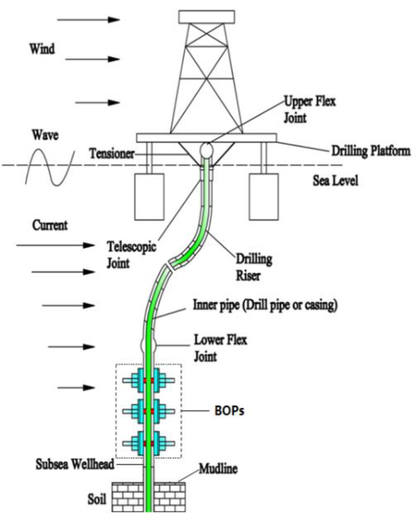
Figure 1. Schematic diagram for typical drilling riser system.
Jmse 10 01627 g001
Figure 2. Typical SW system.
Jmse 10 01627 g002
Figure 3. Architecture of MLP to develop BRANN-based models.
Jmse 10 01627 g003
Figure 4. Framework for predicting the fatigue failure probability of SW.
Jmse 10 01627 g004
Figure 5. Load–stress curve.
Jmse 10 01627 g005
Figure 6. Cyclic dynamic load of SW (HS = 3.25 m, TP = 9.5 s).
Jmse 10 01627 g006
Figure 7. Stress-time curve (HS = 3.25 m, TP = 9.5 s).
Jmse 10 01627 g007
Figure 8. Fatigue damage of SW (HS = 3.25 m, TP = 9.5 s).
Jmse 10 01627 g008
Figure 9. Robustness analysis of BRANN-FD models under varied hidden neuron numbers. (a) HW. (b) LW.
Jmse 10 01627 g009
Figure 10. PDF of fatigue damage of HW weld. (a) Weibull distribution. (b) Lognormal distribution.
Jmse 10 01627 g010aJmse 10 01627 g010b
Figure 11. PDF of fatigue damage of LW weld. (a) Weibull distribution. (b) Lognormal distribution.
Jmse 10 01627 g011
Figure 12. PDF of fatigue damage estimated by KDE. (a) HW. (b) LW.
Jmse 10 01627 g012aJmse 10 01627 g012b
Figure 13. Comparison of parametric and non-parametric estimation results. (a) HW. (b) LW.
Jmse 10 01627 g013aJmse 10 01627 g013b
Figure 14. Relationship between the fatigue failure probability and accumulation fatigue damage.
Jmse 10 01627 g014
Table 1. Parameters of SS10 SW.
ParametersType/mMax O.D/mMin I.D/mHeight/mWeight/kgBending Capacity/Nm
HW0.4760.8510.4461.4762653.567.797 × 106
LW0.7620.9460.6850.762850.54.204 × 106
Table 2. Drilling riser configuration.
Name Number/PieceName Number/Piece
Upper flex joint 1Slip joint1
Telescopic joint1Lower flex joint1
Pup joint1BOPs1
Buoyancy riser joints26SW1
Table 3. Wave scatter diagram of the South China Sea.
Hs/mTp/s
3.54.55.56.57.58.59.510.511.512.513.514.515.516.5
0.250.010.040.090.060.070.070.130.03
0.750.111.13.43.72.91.81.11.20.440.230.130.090.070.08
1.250.010.393.66.75.552.20.910.420.350.240.230.350.11
1.75 0.010.6256.631.60.610.240.210.210.160.260.13
2.25 0.010.011.35.7410.60.240.160.160.160.210.14
2.75 0.142.251.10.30.120.10.090.120.110.09
3.25 0.010.263.11.90.250.110.050.070.060.10.08
3.75 0.040.9220.440.070.030.020.040.050.07
4.25 0.010.151.20.720.060.020.010.030.040.04
4.75 0.040.460.70.070.010.010.010.020.02
5.25 0.010.110.470.080.010.010.010.010.01
5.75 0.010.040.150.120.020.010.010.010.01
6.25 0.020.030.090.010.010.010.010.01
6.75 0.010.020.030.020.010.010.010.01
7.25 0.010.020.020.010.010.010.010.01
7.75 0.010.010.010.010.01
Table 4. Calculation results of beam and spring properties.
Hst/mH/mEI/Nm2Spring Stiffness/N/m
0.510.67.6 × 1081.36 × 107
Table 5. Optimal evaluation results for different random variables distribution types.
Random VariablesDistributionParameters
Significant wave height Weibull k = 1.837 λ = 2.225
Wave periodLognormal μ = 1.94 + 0.0702 H s 1.135 σ = 0.308 exp ( 0.2087 H s ) + 0.000418 exp ( 0.9397 H s )
Table 6. Parameters of PDF for well completion and workover.
Working ConditionDrillingWell CompletionWorkover
Parameters μ −1.906−1.514−1.565
Parameters σ 0.0360.0360.036
Publisher’s Note: MDPI stays neutral with regard to jurisdictional claims in published maps and institutional affiliations.