
Land Subsidence Evolution and Simulation in the Western Coastal Area of Bohai Bay, China

 ,
, 

Abstract
:1. Introduction
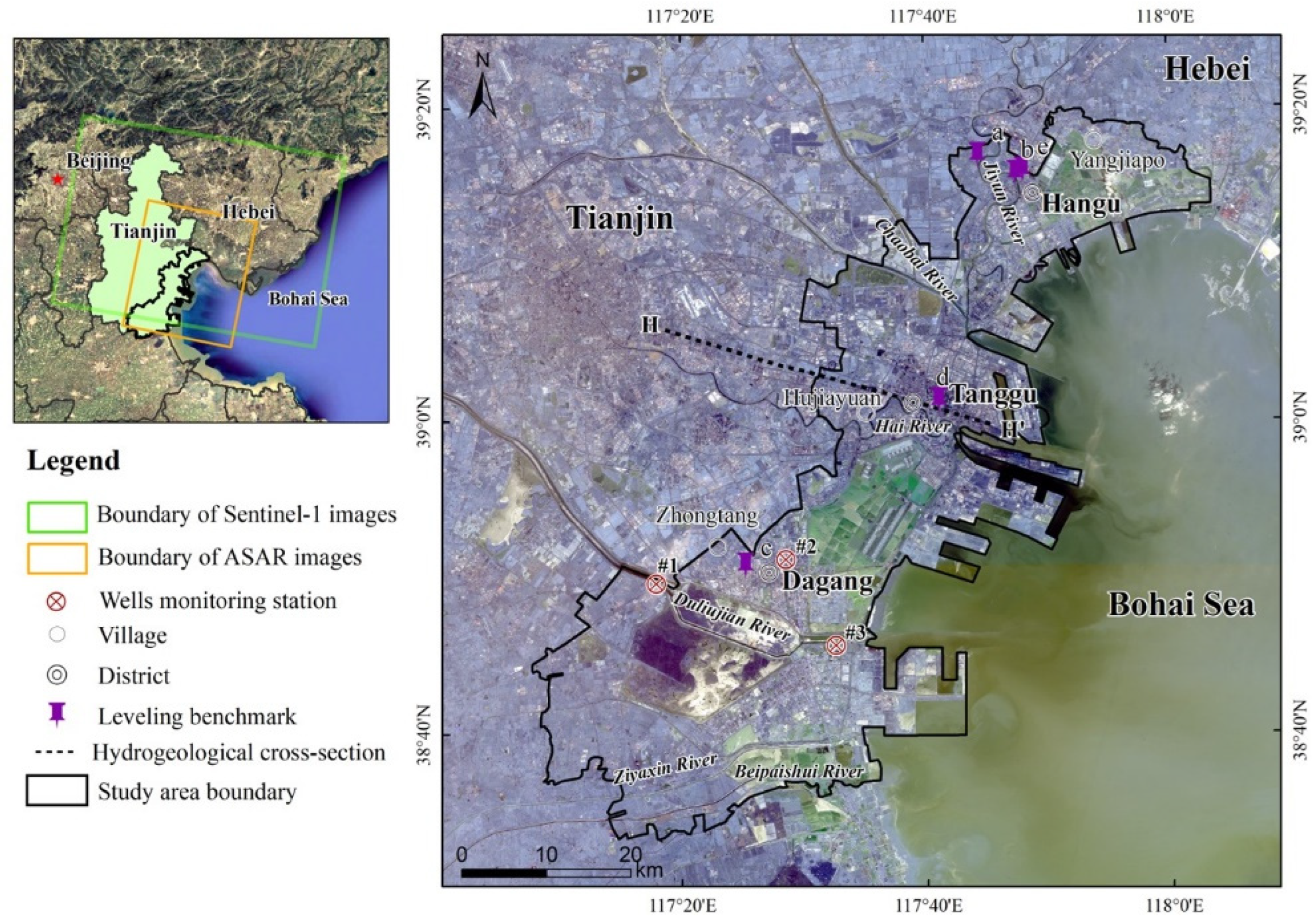
2. Study Area
3. Materials and Methods
3.1. Materials
3.2. Dataset
3.2.1. Remote Sensing Data
3.2.2. Thematic Data
3.3. Methodology
3.3.1. Land Subsidence from 2003 to 2010 with SBAS Technology
3.3.2. Land Subsidence from 2015 to 2020 with PSI Technology
3.3.3. Building Information Using the GEE
3.3.4. Modeling Land Subsidence Based on the GRU
4. Results
4.1. Land Subsidence Distribution and Validation
4.2. Area Occupied by Buildings and Validation
5. Discussion
5.1. Relationships between Factors and Land Subsidence
5.1.1. The Groundwater Level and Land Subsidence
5.1.2. Area Occupied by Buildings and Land Subsidence
5.1.3. Compressible Layer Thickness and Land Subsidence
5.2. Simulation of Land Subsidence
5.2.1. Construction of the GRU Model
5.2.2. Model Validation
6. Conclusions
Author Contributions
Funding
Institutional Review Board Statement
Informed Consent Statement
Data Availability Statement
Acknowledgments
Conflicts of Interest
References
- Herrera-García, G.; Ezquerro, P.; Tomás, R.; Béjar-Pizarro, M.; López-Vinielles, J.; Rossi, M.; Mateos Rosa, M.; Carreón-Freyre, D.; Lambert, J.; Teatini, P.; et al. Mapping the global threat of land subsidence. Science 2021, 371, 34–36. [Google Scholar] [CrossRef] [PubMed]
- Hu, B.; Zhou, J.; Xu, S.; Chen, Z.; Wang, J.; Wang, D.; Wang, L.; Guo, J.; Meng, W. Assessment of hazards and economic losses induced by land subsidence in Tianjin Binhai new area from 2011 to 2020 based on scenario analysis. Nat. Hazards 2013, 66, 873–886. [Google Scholar] [CrossRef]
- Felsenstein, D.; Lichter, M. Social and economic vulnerability of coastal communities to sea-level rise and extreme flooding. Nat. Hazards 2014, 71, 463–491. [Google Scholar] [CrossRef]
- Haley, M.; Ahmed, M.; Gebremichael, E.; Murgulet, D.; Starek, M. Land subsidence in the texas coastal bend: Locations, rates, triggers, and consequences. Remote Sens. 2022, 14, 192. [Google Scholar] [CrossRef]
- Ferretti, A.; Prati, C.; Rocca, F. Nonlinear Subsidence Rate Estimation Using Permanent Scatterers in Differential SAR Interferometry. IEEE Trans. Geosci. Remote Sens. 2000, 38, 2202–2212. [Google Scholar] [CrossRef] [Green Version]
- Berardino, P.; Fornaro, G.; Lanari, R.; Sansosti, E. A New Algorithm for Surface Deformation Monitoring Based on Small Baseline Differential SAR Interferograms. IEEE Trans. Geosci. Remote Sens. 2002, 40, 2375–2383. [Google Scholar] [CrossRef] [Green Version]
- Teatini, P.; Strozzi, T.; Tosi, L.; Wegmüller, U.; Werner, C.; Carbognin, L. Assessing short-and long-time displacements in the Venice coastland by synthetic aperture radar interferometric point target analysis. J. Geophys. Res. Earth Surf. 2007, 112, F01012. [Google Scholar] [CrossRef] [Green Version]
- Ng, A.H.-M.; Ge, L.; Li, X.; Abidin, H.Z.; Andreas, H.; Zhang, K. Mapping land subsidence in Jakarta, Indonesia using persistent scatterer interferometry (PSI) technique with ALOS PALSAR. Int. J. Appl. Earth Obs. Geoinf. 2012, 18, 232–242. [Google Scholar] [CrossRef]
- Lu, W.; Han, C.; Yue, X.; Zhao, Y.; Zhou, G. Land Subsidence Monitoring in Tianjin with PS-InSAR Technique based on Sentinel -1 Data. Remote Sens. Technol. Appl. 2020, 35, 8. [Google Scholar]
- Huang, X.M.; Guo, Q.Q.; Wen, F.T. Land Subsidence Monitoring in Tianjin Binhai New Area Based on Sentinel-1 Data. J. Beijing Polytech. Coll. 2019, 18, 5. [Google Scholar] [CrossRef]
- Törnqvist, T.E.; Wallace, D.J.; Storms, J.E.; Wallinga, J.; Van Dam, R.L.; Blaauw, M.; Derksen, M.S.; Klerks, C.J.; Meijneken, C.; Snijders, E. Mississippi Delta subsidence primarily caused by compaction of Holocene strata. Nat. Geosci. 2008, 1, 173–176. [Google Scholar] [CrossRef]
- Teatini, P.; Tosi, L.; Strozzi, T. Quantitative evidence that compaction of Holocene sediments drives the present land subsidence of the Po Delta, Italy. J. Geophys. Res. Solid Earth 2011, 116, B08407. [Google Scholar] [CrossRef]
- Qu, F.F.; Lu, Z.; Zhang, Q.; Bawden, G.W.; Kim, J.W.; Zhao, C.Y.; Qu, W. Mapping ground deformation over Houston–Galveston, Texas using multi-temporal InSAR. Remote Sens. Environ. 2015, 169, 290–306. [Google Scholar] [CrossRef]
- Van Asselen, S.; Erkens, G.; Stouthamer, E.; Woolderink, H.A.; Geeraert, R.E.; Hefting, M.M. The relative contribution of peat compaction and oxidation to subsidence in built-up areas in the Rhine-Meuse delta, The Netherlands. Sci. Total Environ. 2018, 636, 177–191. [Google Scholar] [CrossRef] [PubMed]
- Wu, T.J.; Cui, X.D. Study and comprehensive treatment of land subsidence in Tianjin. Hydrogeol. Eng. Geol. 1998, 25, 4. [Google Scholar]
- Zhang, T.X.; Shen, W.B.; Wu, W.H.; Zhang, B.; Pan, Y.J. Recent surface deformation in the Tianjin area revealed by Sentinel-1A data. Remote Sens. 2019, 11, 130. [Google Scholar] [CrossRef] [Green Version]
- Guo, J.M.; Hu, J.Y.; Li, B.; Zhou, L.; Wang, W. Land subsidence in Tianjin for 2015 to 2016 revealed by the analysis of Sentinel-1A with SBAS-InSAR. J. Appl. Remote Sens. 2017, 11, 026024. [Google Scholar] [CrossRef]
- Yang, J.; Cao, G.; Han, D.; Yuan, H.; Hu, Y.; Shi, P.; Chen, Y. Deformation of the aquifer system under groundwater level fluctuations and its implication for land subsidence control in the Tianjin coastal region. Environ. Monit. Assess. 2019, 191, 1–14. [Google Scholar] [CrossRef]
- Zhu, L.; Gong, H.L.; Li, X.J.; Li, Y.Y.; Su, X.S.; Guo, G.X. Comprehensive analysis and artificial intelligent simulation of land subsidence of Beijing, China. Chin. Geogr. Sci. 2013, 23, 237–248. [Google Scholar] [CrossRef]
- Shi, L.Y.; Gong, H.L.; Chen, B.B.; Zhou, C.F. Land Subsidence Prediction Induced by Multiple Factors Using Machine Learning Method. Remote Sens. 2020, 12, 4044. [Google Scholar] [CrossRef]
- Hochreiter, S.; Schmidhuber, J. Long short-term memory. Neural Comput. 1997, 9, 1735–1780. [Google Scholar] [CrossRef] [PubMed]
- Cho, K.; Van Merriënboer, B.; Gulcehre, C.; Bahdanau, D.; Bougares, F.; Schwenk, H.; Bengio, Y. Learning phrase representations using RNN encoder-decoder for statistical machine translation. arXiv 2014, arXiv:1406.1078. [Google Scholar] [CrossRef]
- Li, H.J.; Zhu, L.; Dai, Z.X.; Gong, H.L.; Guo, T.; Guo, G.X.; Wang, J.B.; Teatini, P. Spatiotemporal modeling of land subsidence using a geographically weighted deep learning method based on PS-InSAR. Sci. Total Environ. 2021, 799, 149244. [Google Scholar] [CrossRef]
- LeCun, Y.; Bengio, Y.; Hinton, G. Deep learning. Nature 2015, 521, 436–444. [Google Scholar] [CrossRef] [PubMed]
- Li, L.B.; GONG, X.N.; Gan, X.L.; Cheng, K.; Hou, Y.M. Prediction of maximum ground settlement induced by shield tunneling based on recurrent neural network. China Civ. Eng. J. 2020, S01, 7. [Google Scholar]
- Hu, R.L.; Yue, Z.Q.; Wang, L.C.; Wang, S.J. Review on current status and challenging issues of land subsidence in China. Eng. Geol. 2004, 76, 65–77. [Google Scholar] [CrossRef]
- Xiao, G.Q. Study on Mechanism of Clayey Soil by High Pressure Consolidation and Process of Land Subsidence: A Case Study of the G2 Geologic Drill-Hole in Tianjin Binhai New Area. Ph.D. Thesis, China University of Geosciences, Wuhan, China, 2014. [Google Scholar]
- Ha, D.; Zheng, G.; Loáiciga, H.A.; Guo, W.; Zhou, H.Z.; Chai, J.C. Long-term groundwater level changes and land subsidence in Tianjin, China. Acta Geotech. 2021, 16, 1303–1314. [Google Scholar] [CrossRef]
- Zhang, Z.J. Atlas of Groundwater Sustainable Utilization in North China Plain, 1st ed.; China Cartographic Publishing House: Beijing, China, 2009. [Google Scholar]
- Dong, K.G.; Wang, W.; Yu, Q.; Lu, Y. History and enlightenment of land subsidence controlling in Tianjin City. Chin. J. Geol. Hazard Control 2008, 19, 6. [Google Scholar] [CrossRef]
- Yi, L.X.; Zhang, F.; Xu, H.; Chen, S.J.; Wang, W.; Yu, Q. Land subsidence in Tianjin, China. Environ. Earth Sci. 2011, 62, 1151–1161. [Google Scholar] [CrossRef]
- Liu, H.P. The study on the land subsidence with the affect of high-rise buildings in Tianjin Binhai New Area. Ph.D. Thesis, Chang’an University, Xi’an, China, 2010. [Google Scholar]
- Ferretti, A.; Prati, C.; Rocca, F. Permanent scatterers in SAR interferometry. IEEE Trans. Geosci. Remote Sens. 2001, 39, 8–20. [Google Scholar] [CrossRef]
- Werner, C.; Wegmuller, U.; Strozzi, T.; Wiesmann, A. Interferometric point target analysis for deformation mapping. In Proceedings of the IGARSS 2003. 2003 IEEE International Geoscience and Remote Sensing Symposium. Proceedings (IEEE Cat. No. 03CH37477), Toulouse, France, 21–25 July 2003; pp. 4362–4364. [Google Scholar]
- Strozzi, T.; Wegmuller, U.; Tosi, L.; Bitelli, G.; Spreckels, V. Land subsidence monitoring with differential SAR interferometry. Photogramm. Eng. Remote Sens. 2001, 67, 1261–1270. [Google Scholar]
- Phan, T.N.; Kuch, V.; Lehnert, L.W. Land Cover Classification using Google Earth Engine and Random Forest Classifier—The Role of Image Composition. Remote Sens. 2020, 12, 2411. [Google Scholar] [CrossRef]
- Beckschäfer, P. Obtaining rubber plantation age information from very dense Landsat TM & ETM+ time series data and pixel-based image compositing. Remote Sens. Environ. 2017, 196, 89–100. [Google Scholar] [CrossRef]
- Richards, D.R.; Belcher, R.N. Global changes in urban vegetation cover. Remote Sens. 2019, 12, 23. [Google Scholar] [CrossRef]
- Terzaghi, K. Principles of soil mechanics, IV—Settlement and consolidation of clay. Eng. News-Rec. 1925, 95, 874–878. [Google Scholar]
- Zhang, Y.Q.; Yang, X.A.; Zhang, H.T. Analysis of factors influencing land subsidence in tianjin coastal zone. Ground Water 2013, 35, 2. [Google Scholar]
- Khakim, M.Y.; Tsuji, T.; Matsuoka, T. Lithology-controlled subsidence and seasonal aquifer response in the Bandung basin, Indonesia, observed by synthetic aperture radar interferometry. Int. J. Appl. Earth Obs. Geoinf. 2014, 32, 199–207. [Google Scholar] [CrossRef]
- Zill, D.G. Advanced Engineering Mathematics; Jones & Bartlett Publishers: Boston, MA, USA, 2020. [Google Scholar]


| Parameter | Initial Learning Rate | Batch Size | Dropout Rate | Optimizer | RNN Units |
|---|---|---|---|---|---|
| Value | 0.001 | 20 | 0.1 | Adam | 16 |
| Monitoring Well | Displacement (mm) | 2019/09 | 2019/10 | 2019/11 | 2019/12 | MAE | RSME |
|---|---|---|---|---|---|---|---|
| #1 | InSAR derived | −61.94 | −53.83 | −58.80 | −65.34 | 4.13 | 5.00 |
| Modeled | −52.97 | −51.68 | −56.43 | −62.30 | |||
| Absolute error | 8.97 | 2.15 | 2.37 | 3.04 | |||
| #2 | InSAR derived | −24.66 | −18.39 | −22.88 | −27.83 | 0.78 | 0.80 |
| Modeled | −23.82 | −19.3 | −22.37 | −28.70 | |||
| Absolute error | 0.84 | 0.91 | 0.51 | 0.87 | |||
| #3 | InSAR derived | −18.42 | −15.70 | −18.95 | −23.81 | 1.65 | 2.07 |
| Modeled | −16.12 | −15.99 | −18.32 | −20.44 | |||
| Absolute error | 2.3 | 0.29 | 0.63 | 3.37 |
Publisher’s Note: MDPI stays neutral with regard to jurisdictional claims in published maps and institutional affiliations. |
© 2022 by the authors. Licensee MDPI, Basel, Switzerland. This article is an open access article distributed under the terms and conditions of the Creative Commons Attribution (CC BY) license (https://creativecommons.org/licenses/by/4.0/).
Share and Cite
Lu, C.; Zhu, L.; Li, X.; Gong, H.; Du, D.; Wang, H.; Teatini, P. Land Subsidence Evolution and Simulation in the Western Coastal Area of Bohai Bay, China. J. Mar. Sci. Eng. 2022, 10, 1549. https://doi.org/10.3390/jmse10101549
Lu C, Zhu L, Li X, Gong H, Du D, Wang H, Teatini P. Land Subsidence Evolution and Simulation in the Western Coastal Area of Bohai Bay, China. Journal of Marine Science and Engineering. 2022; 10(10):1549. https://doi.org/10.3390/jmse10101549
Chicago/Turabian StyleLu, Can, Lin Zhu, Xiaojuan Li, Huili Gong, Dong Du, Haigang Wang, and Pietro Teatini. 2022. "Land Subsidence Evolution and Simulation in the Western Coastal Area of Bohai Bay, China" Journal of Marine Science and Engineering 10, no. 10: 1549. https://doi.org/10.3390/jmse10101549
APA StyleLu, C., Zhu, L., Li, X., Gong, H., Du, D., Wang, H., & Teatini, P. (2022). Land Subsidence Evolution and Simulation in the Western Coastal Area of Bohai Bay, China. Journal of Marine Science and Engineering, 10(10), 1549. https://doi.org/10.3390/jmse10101549