Article

A Method for Vessel’s Trajectory Prediction Based on Encoder Decoder Architecture

1
Provincial Key Laboratory of Network-Based Intelligent Computing, School of Information Science and Engineering, University of Jinan, Jinan 250022, China
2
School of Information Science and Engineering, Chongqing JiaoTong University, Chongqing 400074, China
*
Authors to whom correspondence should be addressed.
J. Mar. Sci. Eng. 2022, 10(10), 1529; https://doi.org/10.3390/jmse10101529
Submission received: 6 October 2022 / Revised: 15 October 2022 / Accepted: 16 October 2022 / Published: 18 October 2022
(This article belongs to the Section Ocean Engineering)

Abstract

:
Data-driven technologies and automated identification systems (AISs) provide unprecedented opportunities for maritime surveillance. As part of enhancing maritime situational awareness and safety, in this paper, we address the issue of predicting a ship’s future trajectory using historical AIS observations. The objective is to use past data in the training phase to learn the predictive distribution of marine traffic patterns and then use that information to forecast future trajectories. To achieve this, we investigate an encoder–decoder architecture-based sequence-to-sequence prediction model and CNN model. This architecture includes a long short-term memory (LSTM) RNN that encodes sequential AIS data from the past and generates future trajectory samples. The effectiveness of sequence-to-sequence neural networks (RNNs) for forecasting future vessel trajectories is demonstrated through an experimental assessment using an AIS dataset.

1. Introduction

Maritime shipping acts as the backbone for thriving economies and international trade. In 2021, global trade reached a value of more than USD 28 trillion, 80% of which was transported by sea. These flourishing trades have a significant influence on the shipping industry. On the positive side, it increases the number of ships contributing to economic growth. At the same time, it also increases the possibility of maritime incidents that lead to casualties, and huge economic and environmental damages. Although there have been advancements in maritime technology and international safety regulations, accidents in the marine industry still occur. About 3000 shipping incidents happened in 2021 alone [1]. In total, 54 vessels were lost and 50% of them were cargo ships, causing millions of dollars of economic damage. South China, Indochina, Indonesia, and the Philippines ranked among the highest for global loss; about one-third of the total losses occurred in this region. Even though machinery damage accounts for the majority of maritime incidents, collision remains one of the top causes of fatal incidents and the ultimate loss of vessels. Ö. Uğurlu [2], in his study, showed that collision and grounding pose the highest risk of economic loss. Multiple studies and surveys from the Japanese government show that human navigational error is the primary (70%) cause of maritime accidents. Automated navigation can contribute to reducing human error and preventing economic loss. Additionally, as the business for autonomous vessels develops, trajectory prediction has become more crucial than ever before.
As Big Data and the Internet of Things (IoTs) technology progress, more and more sensors are being deployed in marine transportation systems. This integration of technologies is expected to reduce maritime accidents and improve safety in maritime environments. A key capability needed to meet those expectations is to predict the future position of vessels. The enormous amount of automatic identification system (AIS) data now makes it possible to analyze and create marine traffic monitoring systems, such as vessel trajectory prediction, threat assessment, anomaly detection, etc. This prediction capability increases maritime situational awareness and reduces the collision possibility for autonomous and non-autonomous vessels, as well as large- and small-sized vessels. It is also crucial for maritime search and rescue (SAR) operations. A recent loss, that could be avoided with an advanced trajectory prediction system, happened in June 2022, wherein an autonomous underwater vehicle (AUV) was lost in Taiwanese waters while it was operating a rescue mission for the crashed fighter jet “Mirage 2000”, causing a loss of 40 million yuan in total. To avoid such economic damage and to facilitate emergency rescue missions, it is paramount to know the probable future trajectory of the vessel.
The automatic identification system (AIS) is a self-reporting system for vessels that was originally created to avoid possible incidents and is now a required feature for international passenger and cargo ships (i.e., ships with a gross tonnage of 300 or larger) [3,4,5]. The AIS system broadcasts information about the vessel at a certain interval (ranging from 2 s to 180 s). In addition, it broadcasts voyage-related information every 6 min [6]. AIS data mainly contain the vessel’s dynamic (the current position according to the latitude and longitude coordinates, the current speed over ground—SOG, the current course over ground–COG, etc.), and static information (identification number in the format maritime mobile service identity—MMSI number, the name of the vessel, etc.) [6].
When it comes to improving safety and reducing accidents, accurate trajectory (path) prediction is a primary concern, both for autonomous vehicles (on-road) and vessels (in oceans). That is why researchers have been recently trying to understand the behavior of autonomous applications. A recent study mentions state-of-the-art methods for that [7]. However, some differences should be considered. On the one hand, vehicles have certain speed limits for different roads, specific driving lanes to follow, and traffic signals, etc. [7] On the other hand, vessels (ships) have no specific speed limits (speed depends on the weather, wind, and water current speed), no lane to follow (for maritime navigation), and maritime waypoints (turning points where car take left or right turn on the road) are less strict [8].
Even though the availability of AIS data presents an opportunity to systematically extract crucial data to improve the safety of marine navigation and situational awareness for rescue operations, accurate vessel trajectory prediction using AIS data remains a challenge due to the variety of behavior exhibited by the ships and the quality of AIS data [9,10]. A typical maritime traffic pattern is shown in Figure 1.
In this study, in contrast to a model-based method, we adopt a data-driven approach to address the vessel trajectory prediction problem. The LSTM encoder–decoder architecture serves as the foundation for our suggested approach, and has emerged as an effective model for sequence-to-sequence learning. The rest of this paper is structured as follows. Section 2 discusses earlier vessel trajectory prediction studies, as well as its benefits and drawbacks. The strategy described in this research is discussed in depth in Section 3. Section 4 explains the experiment’s data preparation technique. Section 5 displays the results of the experiment, as well as a comparison to other models. Finally, Section 6 concludes the paper.

2. Related Work

Predicting a ship’s trajectory using AIS data is commonly referred to as a regression problem and uses a series of past AIS observations of the ship to predict its future position. Several approaches have been proposed [11,12]. In the simplest models, conventional interpolation methods such as linear interpolation and curved interpolation are used. More sophisticated models construct the ship’s kinematic equations and assimilate AIS observations using extended Kalman filters [13] and particle filters. Among the model-based predictors, the simplest and probably the most popular is the near-constant velocity (NCV) linear model [14]. The NCV model has an underlying robustness to the quality of the input data and the capacity to forecast short-term linear trajectories. The NCV model tends to exaggerate the level of forecast uncertainty as the time horizon increases, making it unsuitable for medium- and long-term forecasting. Recent research has suggested a slightly more sophisticated ship prediction model based on the Ornstein–Uhlenbeck (OU) stochastic process. This model has been demonstrated to be especially effective for non-maneuvering motion and large forecast time frames [15]. The OU model was integrated with data-driven techniques to create unsupervised processes that automatically extract knowledge about marine traffic patterns [16,17]. The OU model has also been applied to detect anomalies at sea [18]. Nonlinear filtering was investigated in further research on AIS-based vessel trajectory predictions [19], nearest-neighbor search methods [20], and machine learning techniques [21].
Deep neural network (NN)-based models have been proven to perform very well on complex tasks such as image processing [22] and speech recognition [23]. However, NNs do not perform well in mapping sequence tasks. This drawback highlights the need to explore a recurrent neural network (RNN) [24], which can remember important things from past inputs, making it very useful for sequential data processing tasks, such as processing time series, text, machine translation tasks, etc. [25]. This allows it to utilize the observed time series to predict the time series of a future horizon. In this case, the larger the future time horizon, the more difficult the problem becomes. RNN-based models use internal memory representation to learn temporal patterns. Modern encoder–decoder architecture-based models (the first RNN encodes an input sequence as a collection of vector representations and the second RNN creates the output sequence) have become the standard approach to sequence-to-sequence processing tasks such as machine translation and audio recognition [26]. Early works in this direction include the use of naïve RNN models and hybrid models using ARIMA and multilayer perceptron, as well as a combination of vanilla RNN and dynamic Boltzmann machines.
Since AIS data are time-series data, in this paper we investigate whether an improved RNN model can be applied to a vessel’s trajectory prediction task. Our proposed method for this paper is built upon LSTM encoder–decoder architecture. Its scalability and capability of handling long-term dependencies [27] make LSTM an ideal choice for our experiment.

3. Our Approach and Other Models

In this section, first we formulate our problem, and then introduce our approached model. Finally, we briefly describe several other neural network models that we compare our results with in the experiment section.

3.1. Problem Formulation

In our setup, we considered the environment as four-dimensional. In addition, ships following nearly the same path will share the same kinematic information, i.e., longitude and latitude. We will also consider other kinematic information, namely COG (course over ground) and SOG (speed over ground). Let us consider P as a time-ordered sequence of observations.
P = S i , T i
where Si is a 4D real-valued feature vector corresponding to latitude and longitude at time T. i = 1, 2, 3, …... N, i, and N represent the index of trajectory and the total number of trajectories, respectively. Ti is the number of AIS messages collected for the i-th trajectory. So, a dataset consisting of total N trajectories can be written as an ordered sequence of tuples P = {(Si, Ti)}Ni=1 where each data case consists of vessel states defined in (1) and Ti = (t0, t1, ……ti) are the time stamps when AIS messages were recorded. Our goal is centered around future trajectory prediction for a vessel and we will use sequence-to-sequence learning to solve the problem. Let us assume that our dataset is regularly sampled by interpolating the original trajectory with a fixed-length sampling time ∆. Now, our target is to learn the function
y k , h = σ l , h x k , l
Mapping an arbitrary input sequence of x k , l containing l states observed up to time step k, to output the sequence of y k , h h steps in the future from step k. The sequence-to-sequence trajectory prediction at time step k can be written mathematically as
y k , h = σ l , h x k , x k 1 , x k 2 , , x k l + 1
where l represents how many lag states were used to predict the target sequence. σ l , h is the unknown function that maps between input and output. Simply put, it is a probabilistic distribution of p ( y | x ) , indicating the predicted future state of y based on known state x .

3.2. Encoder–Decoder Architecture

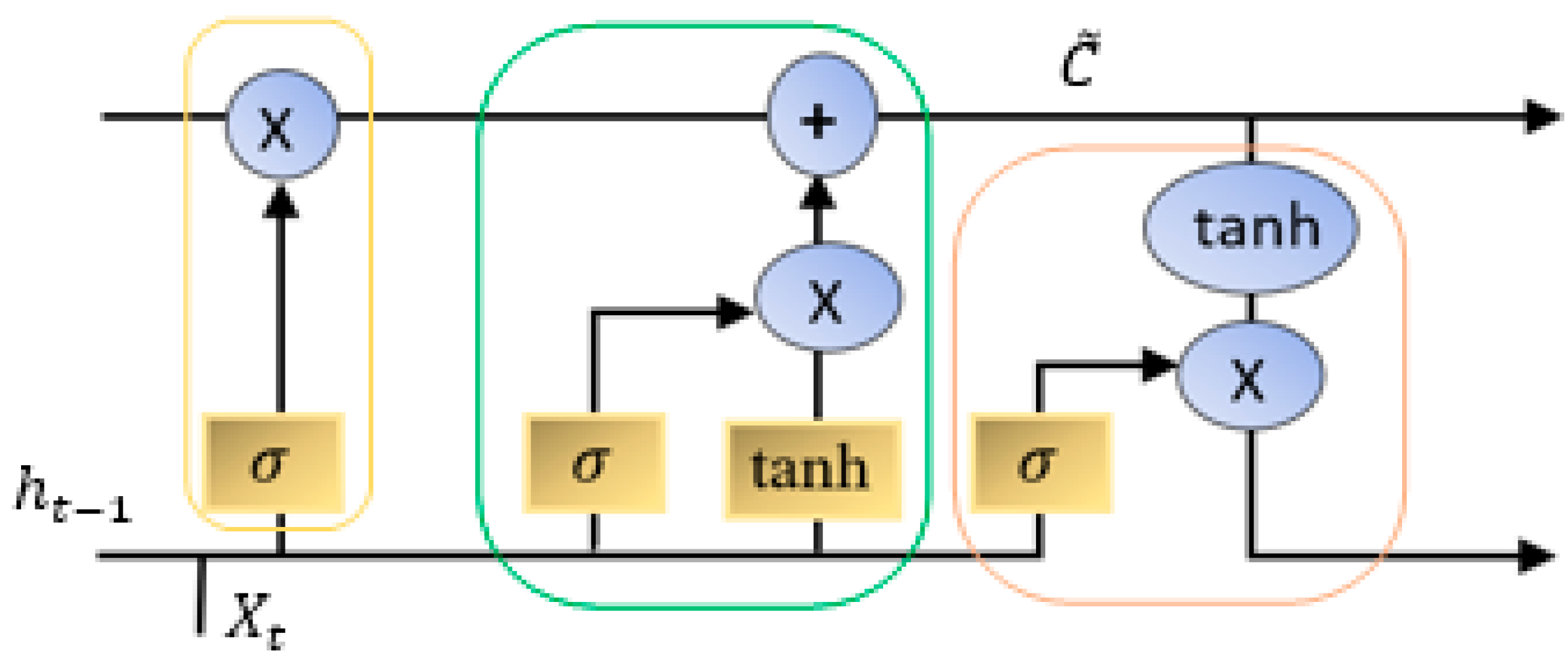
A special type of artificial recurrent neural network (RNN) called long short-term memory (LSTM) is used in deep learning to learn long-term sequence dependency among a dataset sequence. A large enough RNN can theoretically store long-term dependencies; however, standard RNN cannot encode past data for very long. Another limitation of standard RNN is it cannot map different lengths of sequence for input and output. LSTM is, in fact, a complex activation unit that solves the standard RNN’s limitations. The repeating module and chain-like structure of LSTMs enable them to retain information for extended periods of time. Indeed, they eliminate long-term dependencies by allowing users to choose which information to remember or to forget. The following equations represent the LSTM module:
f t = σ W f × C t 1 , h t 1 , x t + b f
i t = σ W i × C t 1 , h t 1 , x t + b f
C ˜ = t a n h W c × h t 1 , x t + b c
o t = σ ( W 0 × C t , h t 1 , x t + b 0
At time step t, x t represents the input, h t 1 represents the hidden state at time step t − 1, and y t is the output. The cell state at time t 1 is C t 1 . The “forget Gate layer,” represented by the yellow unit, selects what needs to be remembered and what can be forgotten. A sigmoid layer and a tanh layer make up the “update layer” in the middle. The sigmoid layer selects the value that will change, and the tanh layer builds a vector of candidate value C ~ t to be added to the state. Now, we can update the cell state C t at time step t . A diagram of LSTM is shown in Figure 2.
C t = f t × C t 1 + i t × C ~ t
Now, we can calculate our output, which will be determined by cell state C t 1 , hidden state h t 1 , and input X t .
o t = σ W 0 × h t 1 , x t + b 0
h t = o t × t a n h C t
o t   represents the part of the cell state that we will output. y t is the output at time step t , as well as the hidden state of that time step.

3.3. Transformer

The Transformer uses the attention mechanism similar to LSTM. It transforms one sequence to another sequence by utilizing the encoder and decoder, but it differs from other sequence-to-sequence models since it does not use any recurrent neural networks. Instead, its architecture makes use of an attention mechanism in a certain way to achieve the result. In Transformer models, both encoder and decoder parts consist of multiple layers of multi-head attention and feed-forward layers [28]. Since it does not use any RNNs, to remember the key part from the input sequence, it uses positional encoding to help produce a better result in the decoding step.
Its encoder and decoder are composed of (Nx) multiple similar stacked layers. As shown in Figure 3, a fully connected feed-forward network and a multi-head self-attention mechanism are included in each layer of the encoder. Every stack of decoders also has a third layer that conducts multi-head attention over the output of the encoder stack, in addition to these two levels.
The attention mechanism can be described by the following equation:
A t t e n t i o n Q , K , V = s o f t m a x ( Q K T D K ) V
where Q is a matrix that contains the query, K are all the keys, and V are the vector representation of the values. 1 D K is the scaling factor.
FFN(x) = max (0; xW1 + b1) W2 + b2
The equation above represents the other part of the stacked layer, a fully connected feed-forward network, which consists of two linear transformations with a ReLU activation between them.

3.4. LSTNet (Long- and Short-Term Time-Series Network)

The long- and short-term time-series network (LSTNet) combines the strengths of the convolutional layer to uncover local dependence patterns among multidimensional input variables and the recurrent layer to capture complicated long-term relationships. Taking advantage of the periodic features of the input time series signals, a recurrent structure helps to capture long-term dependency patterns and simplifies optimization. In addition, the LSTNet also includes a conventional autoregressive linear model in addition to the non-linear neural network component, as shown in Figure 4, making the non-linear deep learning model more robust for time series with large scale shifting [29]. Overall, convolution neural networks (CNNs) and recurrent neural networks (RNNs) are used by the LSTNet to extract short-term local dependency patterns between variables and to find long-term patterns for time series.

4. AIS Data Preparation

Different studies, including one by Karahalios, show that about 49% of incidents happen in coastal areas [30] (27% near the coast and 22% in narrow channels), while another study by Japan [31] shows that about 90% of maritime accidents happen within 37 km (20 NM) of the shore. Since our study contributes to improve maritime safety, we initially focused our experiment on coastal areas. We conducted experiments on a real-world AIS dataset from the East China Sea which contains about 125 K irregularly sampled AIS data recorded during July–August 2021 from 200 different vessel journeys. The observed trajectories reflect several marine route patterns with many waypoints. We retrieved four typical ship trajectories (i.e., four groups of AIS data samples) from the observed navigation zone for our experimental evaluation. Case 1, Case 2, Case 3, and Case 4 were picked from the above-mentioned dataset based on the ship’s MMSI number. These four retrieved trajectories represent the water of the Yangtze River estuary. Vessel traffic regulation and safety management for this area of water are governed by the Shanghai Maritime Safety Administration. For all vessels, it is mandatory to follow ‘The Ships’ Routeing System in Yangtze Estuary—2008′ which is formulated in accordance with Traffic Separation Scheme (TSS). In the first phase of the experiment, we used the Case 1 and 2 trajectories, and Cases 3 and 4 were used for the second phase of the experiment. Since both ship longitudes and latitudes shifted in a limited range, the spatial–temporal ship trajectory distribution represented in Figure 5 indicates that the ship traveled back and forth in a narrow region. However, the raw ship trajectory data revealed a significant number of outliers. Various abnormal ship positions from the data samples stood out in particular because they were a great distance from their nearby neighbors and suggested an unjustified ship displacement.
We removed the inappropriate speed and position data, and removed abnormal messages (we considered an AIS message as abnormal if the empirical speed is unrealistic). We then made calculations by dividing the distance traveled by the corresponding interval between two consecutive messages, which we considered to be 20 knots. With a fixed-length sampling time of = 2 min, we resampled the original AIS trajectories and retrieved around 1.5 k four-dimensional time-ordered features (latitude–longitude–SOG–COG). Then, using a five-fold cross-validation technique, we created the training/validation trajectory dataset. Finally, we rescaled the features in the training set using standardization (z-score normalization) before feeding them into the model. The model has to learn to predict a target sequence of length h based on an input sequence of length l; thus, we extracted all the time windows of size l + h that were available.

5. Experimental Setup and Result

In this experiment, the multi-variate input sequences were initially transferred into 64 cells for encoding using an LSTM encoder–decoder architecture. Following that, the output sequence was gradually decoded. The learning rate for the prediction network’s Adam optimizer training was set to 0.001, the batch size was 32, and the maximum number of epochs was 160. According to the experimental findings, the sequence-to-sequence model can be a useful tool for predicting vessel trajectories. For a fixed-length output sequence with l = 20 (previous steps) and h = 2 (future steps), the effectiveness of an LSTM-based technique was assessed. LSTM configuration of our experiment is shown in Table 1.
For an in-depth comparison, we compared our experiment with several other good performing time-series prediction models in the deep learning field. We used the transformer, LSTNet, CNN, and GRU model-based prediction strategy. With the same configuration as the LSTM model, we trained these models with an Adam optimizer with learning rate r = 0.001, as illustrated in Table 2. It is important to note that, based on the early findings, this should be viewed as a qualitative comparison.
Additionally, the dataset was divided into training, validation, and test sets before the network was trained. The training outcome of the LSTM model is represented in Figure 6 for clarity. It seems that both the training and validation losses are less until about 80 iterations. It was determined that the model had converged at this moment as a result.
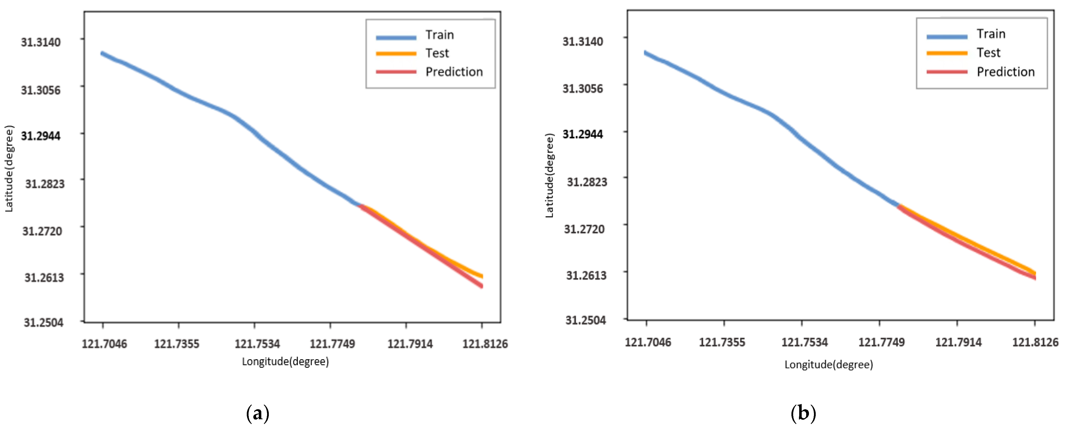
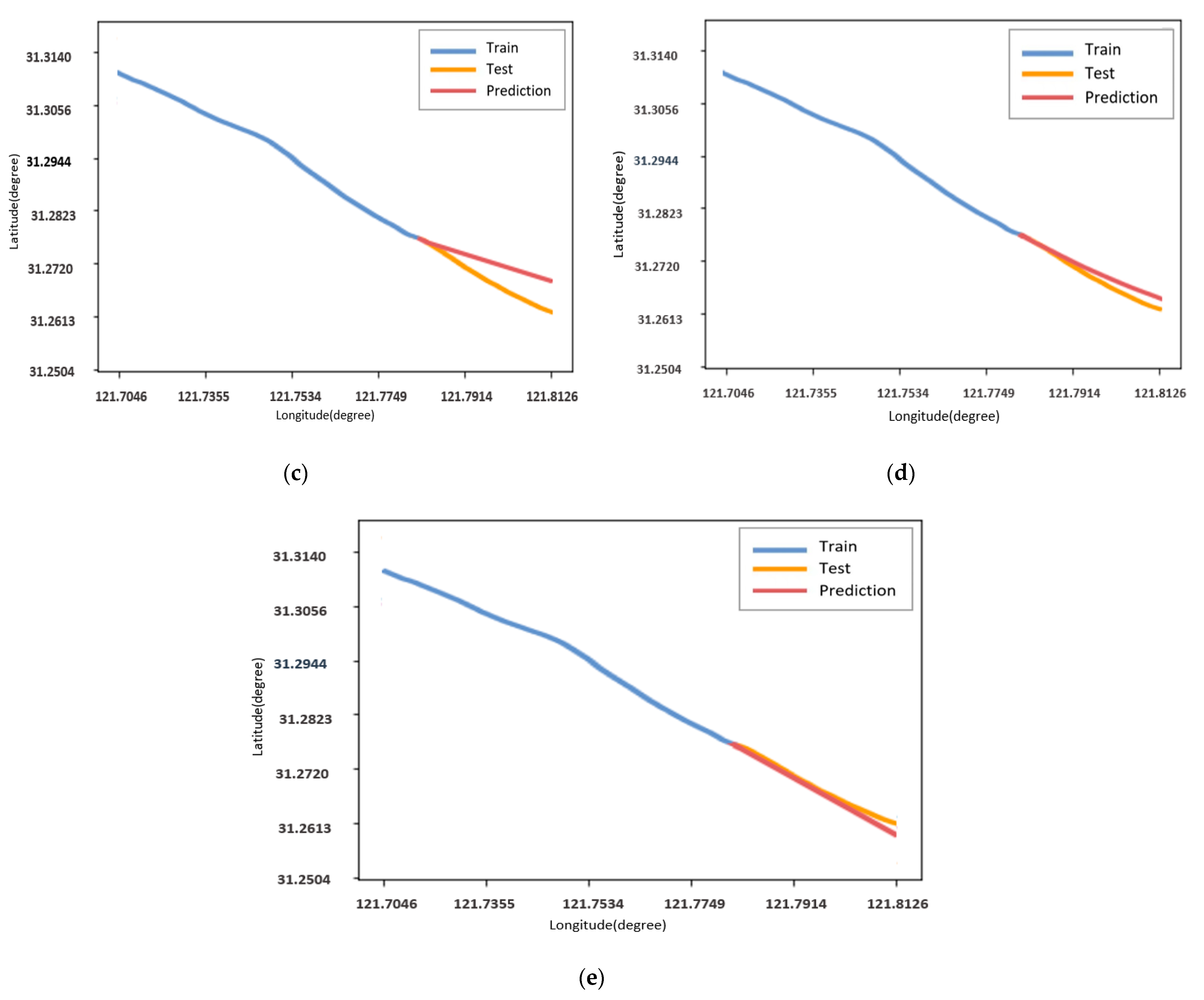
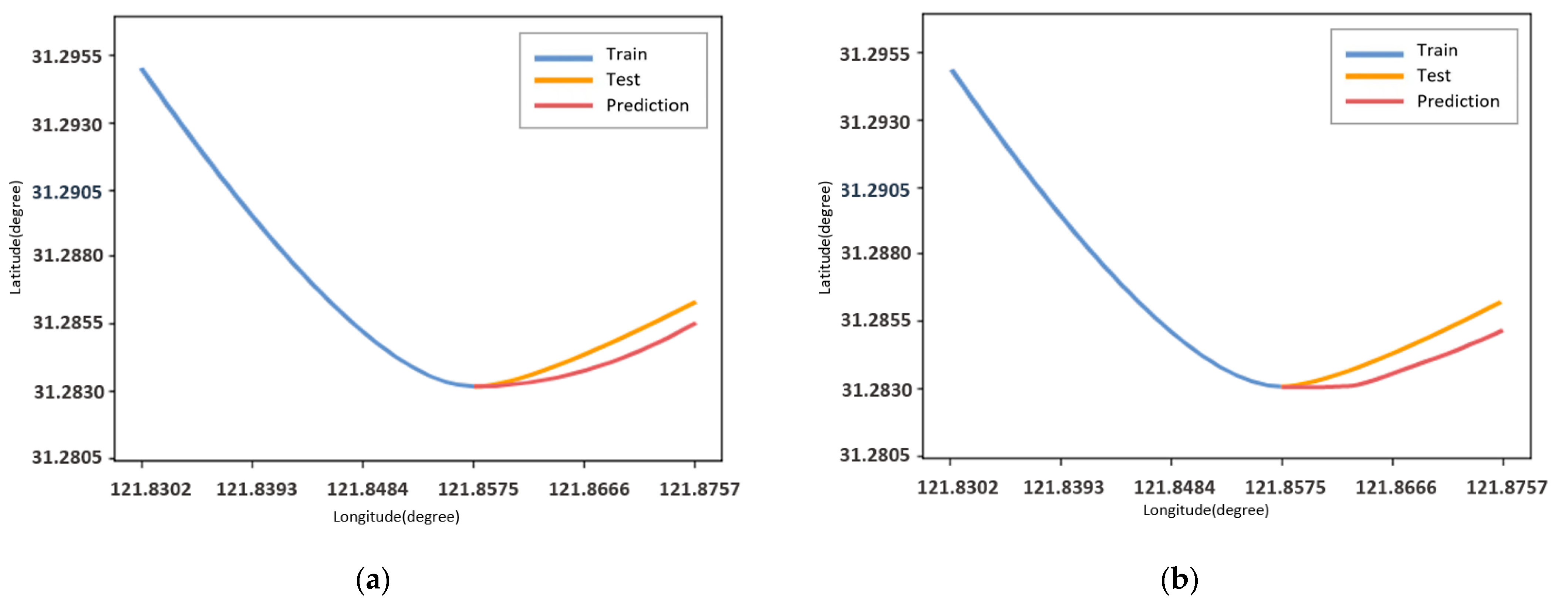
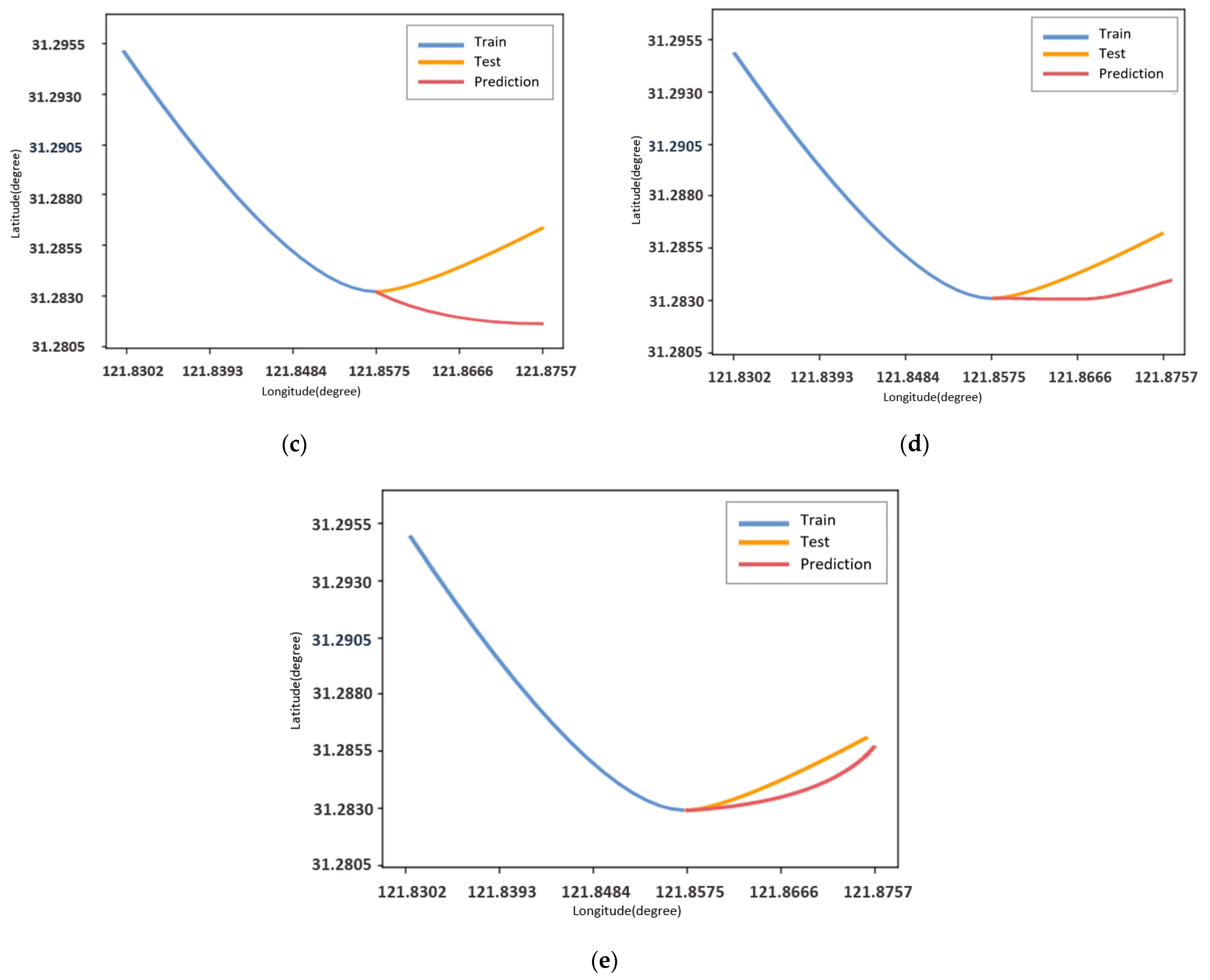
Figure 7 and Figure 8 show that for a fixed-length output, all the models performed reasonably well with straight-path prediction, but struggled to predict waypoints. In waypoints, while examining the variable output steps, we noticed that CNN and LSTM models caught up with the prediction after a few steps, while GRU produced the worst result. To evaluate the output results of those models, we adopted the root means squared error (RMSE) and mean absolute error (MAE) calculation.
RMSE = 1 N t h o u t p u t t h a c t u a l t 2 MAE = 1 N t h o u t p u t t h a c t u a l t
where h o u t p u t t is the predicted vessel trajectory position at time step t, and h a c t u a l t is the original trajectory position of the vessel at time step t. These metric scores are negatively oriented; the lower score output, the better the model. In other words, the lower the model scores, the more accurate prediction it can make relative to its original trajectory.
After evaluating the experimental results, they reflect that the LSTNet and Transformer models both tend to produce more accurate results. However, when compared to LSTM, LSTNet, and CNN models, the Transformer’s attention mechanism adds more weight to the model, resulting in a much longer training time. It also performs even less efficiently than the LSTM and CNN models when combined with less layers. LSTNet’s advantage is in its CNN module which reduces parameters, thus making it faster to train than Transformer. Table 3 also shows that for the fixed-length output produced with LSTM and CNN models, the prediction error range is very close to each other, and overall preforms better than the GRU model. In Table 4, we reduced our input steps (l) down to 10 time steps, which is worth 20 min of past trajectory, and increased the output (h) time steps to 4 time steps.
Analyzing the outcome of the experiment, we noticed that a reduction in the input sequence had a negligible influence on the models when predicting the straight-line navigation trajectory. Influence may increase if we further reduce the input size. For waypoint navigation, we saw relatively worse prediction performance from all models. However, for LSTNet, and Transformer, this influence is significantly less when compared to other models. Table 4 also indicates that the frequency of error variance increases as the number of future time steps increase. For the second phase of the experiment, we considered the LSTM and CNN models, which produced satisfactory results while being more lightweight. We proceeded with our experiment using Case 3 and Case 4 trajectories, as mentioned in the data-processing part.
Figure 9 shows the number of actual trainable parameters of both models. CNN and LSTM have 2257 and 17,425 parameters, respectively. This suggests that the CNN model is significantly lighter than the LSTM one and easier to train.
Table 5 indicates the close prediction result by both the CNN and LSTM models on Case 3 and 4 trajectory sets from the East China Sea.
Figure 10 shows the prediction performance of LSTM and CNN models on the test data of Case 3 and Case 4, qualitatively corresponding to the true trajectory. The orange line represents the actual trajectory of the vessel. The blue and purple colors represent CNN and LSTM model predictions on test data, respectively. Figure 10 also illustrates the prediction deviation in major waypoint areas. In our experiment, we observed that a comparatively light CNN model with fewer parameters can predict trajectory very similarly to the LSTM model. We also observed that our model performs better with a longer l (past steps) range. This might be a limitation of using LSTM architecture where all necessary information is extracted from limited input sequences and can be a bottleneck in improving performance.

6. Conclusions

We explored the encoder–decoder architecture-based LSTM model for vessel trajectory prediction. With our AIS datasets, the prediction result was consistent with true trajectory, except for waypoints, where the predictions were relatively less consistent when there was a major turning point in the original trajectory. We also found that the Transformer model and LSTNet produce better results but have a longer training time. A clustering approach on the training dataset might improve the prediction performance for both LSTM- and CNN-based models. Besides that, a relatively lightweight CNN model can be used in future trajectory predictions, as it produces a significantly better result with fewer parameters. In future work, we will aim to improve the prediction time window with a lightweight model, and prediction accuracy around waypoints.

Author Contributions

Conceptualization, M.M.B. and J.Z.; methodology, M.M.B. and J.Z.; software, M.M.B.; validation, M.M.B., J.Z. and T.Z.; formal analysis, M.M.B.; data curation, M.M.B.; writing—original draft preparation, M.M.B.; writing—review and editing, M.M.B., J.Z. and T.Z; supervision, J.Z. and T.Z; funding acquisition, J.Z. All authors have read and agreed to the published version of the manuscript.

Funding

This work is supported by (1) 2021–2023 National Natural Science Foundation of China under Grant (Youth) No. 52001039; (2) 2022–2025 National Natural Science Foundation of China under Grant No. 52171310; (3) 2020–2022 Funding of the Shandong Natural Science Foundation in China under Grant No. ZR2019LZH005; (4) 2022–2023 Research fund from Science and Technology on Underwater Vehicle Technology Laboratory under Grant 2021JCJQ-SYSJJ-LB06903.

Conflicts of Interest

The authors declare no conflict of interest.

References

  1. Available online: https://www.agcs.allianz.com/news-and-insights/reports/shipping-safety.html#download (accessed on 15 October 2022).
  2. Özkan, U.; Erol, S.; Başar, E. The analysis of life safety and economic loss in marine accidents occurring in the Turkish Straits. Marit. Policy Manag. 2016, 43, 356–370. [Google Scholar]
  3. Chen, X.; Wang, S.; Shi, C.; Wu, H.; Zhao, J.; Fu, J. Robust ship tracking via multi-view learning and sparse representation. J. Navig. 2019, 72, 176–192. [Google Scholar] [CrossRef]
  4. Chen, X.; Xu, X.; Yang, Y.; Wu, H.; Tang, J.; Zhao, J. Augmented ship tracking under occlusion conditions from maritime surveillance videos. IEEE Access 2020, 8, 42884–42897. [Google Scholar] [CrossRef]
  5. Fang, Z.; Jian-Yu, L.; Jin-Jun, T.; Xiao, W.; Fei, G. Identifying activities and trips with GPS data. IET Intell. Transp. Syst. 2018, 12, 884–890. [Google Scholar] [CrossRef]
  6. Available online: https://artes.esa.int/satellite-%E2%80%93-automatic-identification-system-satais-overview (accessed on 30 July 2022).
  7. Mozaffari, S.; Al-Jarrah, O.Y.; Dianati, M.; Jennings, P.; Mouzakitis, A. Deep learning-based vehicle behavior prediction for autonomous driving applications: A review. IEEE Trans. Intell. Transp. Syst. 2020, 23, 33–47. [Google Scholar] [CrossRef]
  8. Available online: https://www.imo.org/en/About/Conventions/Pages/COLREG.aspx (accessed on 13 July 2022).
  9. Bye, R.J.; Almklov, P.G. Normalization of maritime accident data using AIS. Mar. Policy 2019, 109, 103675. [Google Scholar] [CrossRef]
  10. Iphar, C.; Ray, C.; Napoli, A. Data integrity assessment for maritime anomaly detection. Expert Syst. Appl. 2020, 147, 113219. [Google Scholar] [CrossRef]
  11. Millefiori, L.M.; Braca, P.; Bryan, K.; Willett, P. Modeling vessel kinematics using a stochastic mean-reverting process for long-term prediction. IEEE Trans. Aerosp. Electron. Syst. 2016, 52, 2313–2330. [Google Scholar] [CrossRef]
  12. Pallotta, G.; Vespe, M.; Bryan, K. Vessel Pattern Knowledge Discovery from AIS Data: A Framework for Anomaly Detection and Route Prediction. Entropy 2013, 15, 2218–2245. [Google Scholar] [CrossRef] [Green Version]
  13. Perera, L.P.; Oliveira, P.; Soares, C.G. Maritime Traffic Monitoring Based on Vessel Detection, Tracking, State Estimation, and Trajectory Prediction. IEEE Trans. Intell. Transp. Syst. 2012, 13, 1188–1200. [Google Scholar] [CrossRef]
  14. Li, X.R.; Jilkov, V.P. Survey of maneuvering target tracking. Part I. Dynamic models. IEEE Trans. Aerosp. Electron. Syst. 2003, 39, 1333–1364. [Google Scholar]
  15. Uney, M.; Millefiori, L.M.; Braca, P. Data driven vessel trajectory forecasting using stochastic generative models. In Proceedings of the IEEE International Conference on Acoustics, Speech and Signal Processing (ICASSP), Brighton, UK, 12–17 May 2019; pp. 8459–8463. [Google Scholar]
  16. Coscia, P.; Braca, P.; Millefiori, L.M.; Palmieri, F.A.N.; Willett, P. Multiple Ornstein–Uhlenbeck processes for maritime traffic graph representation. IEEE Trans. Aerosp. Electron. Syst. 2018, 54, 2158–2170. [Google Scholar] [CrossRef]
  17. Forti, N.; Millefiori, L.M.; Braca, P. Unsupervised extraction of maritime patterns of life from Automatic Identification System data. In Proceedings of the IEEE/MTS OCEANS, Marseille, France, 17–20 June 2019. [Google Scholar]
  18. Forti, N.; Millefiori, L.M.; Braca, P.; Willett, P. Anomaly detection and tracking based on mean–reverting processes with unknown parameters. In Proceedings of the IEEE International Conference on Acoustics, Speech and Signal Processing (ICASSP), Brighton, UK, 12–17 May 2019; pp. 8449–8453. [Google Scholar]
  19. Mazzarella, F.; Arguedas, V.F.; Vespe, M. Knowledge-based vessel position prediction using historical AIS data. In Proceedings of the Sensor Data Fusion: Trends, Solutions, Applications, Bonn, Germany, 6–8 October 2015. [Google Scholar]
  20. Hexeberg, S.; Flaten, A.L.; Eriksen, B.H.; Brekke, E.F. AIS-based vessel trajectory prediction. In Proceedings of the International Conference on Information Fusion, Xi’an, China, 10–13 July 2017. [Google Scholar]
  21. Nguyen, D.; Vadaine, R.; Hajduch, G.; Garello, R.; Fablet, R. A multi-task deep learning architecture for maritime surveillance using AIS data streams. In Proceedings of the IEEE International Conference on Data Science and Advanced Analytics, Turin, Italy, 1–3 October 2018; pp. 331–340. [Google Scholar]
  22. Zhou, T.; Li, Z.; Zhang, C.; Ma, H. Classify multi-label images via improved CNN model with adversarial network. Multimed. Tools Appl. 2020, 79, 6871–6890. [Google Scholar] [CrossRef]
  23. Khalil, R.A.; Jones, E.; Babar, M.I.; Jan, T.; Zafar, M.H.; Alhussain, T. Speech Emotion Recognition Using Deep Learning Techniques: A Review. IEEE Access 2019, 7, 117327–117345. [Google Scholar] [CrossRef]
  24. Available online: https://builtin.com/data-science/recurrent-neural-networks-and-lstm (accessed on 15 October 2022).
  25. Fujita, T.; Luo, Z.; Quan, C.; Mori, K. Simplification of RNN and Its Performance Evaluation in Machine Translation. Transactions of the Institute of Systems. Control Inf. Eng. 2020, 33, 267–274. [Google Scholar]
  26. Singh, S.P.; Kumar, A.; Darbari, H.; Singh, L.; Rastogi, A.; Jain, S. Machine translation using deep learning: An overview. In Proceedings of the 2017 International Conference on Computer, Communications and Electronics (Comptelix), Jaipur, India, 1–2 July 2017. [Google Scholar]
  27. Hochreiter, S.; Schmidhuber, J. Long short-term memory. Neural Comput. 1997, 9, 1735–1780. [Google Scholar] [CrossRef] [PubMed]
  28. Vaswani, A.; Shazeer, N.; Parmar, N.; Uszkoreit, J.; Jones, L.; Gomez, A.N.; Kaiser, Ł.; Polosukhin, I. Attention is all you need. Adv. Neural Inf. Process. Syst. 2017, 30. [Google Scholar] [CrossRef]
  29. Lai, G.; Chang, W.C.; Yang, Y.; Liu, H. Modeling long-and short-term temporal patterns with deep neural networks. In Proceedings of the 41st International ACM SIGIR Conference on Research & Development in Information Retrieval, Ann Arbor, MI, USA, 8–12 July 2018. [Google Scholar]
  30. Karahalios, H. The contribution of risk management in ship management: The case of ship collision. Saf. Sci. 2014, 63, 104–114. [Google Scholar] [CrossRef]
  31. Available online: https://www8.cao.go.jp/koutu/kihon/keikaku8/english/part2.html (accessed on 10 October 2022).
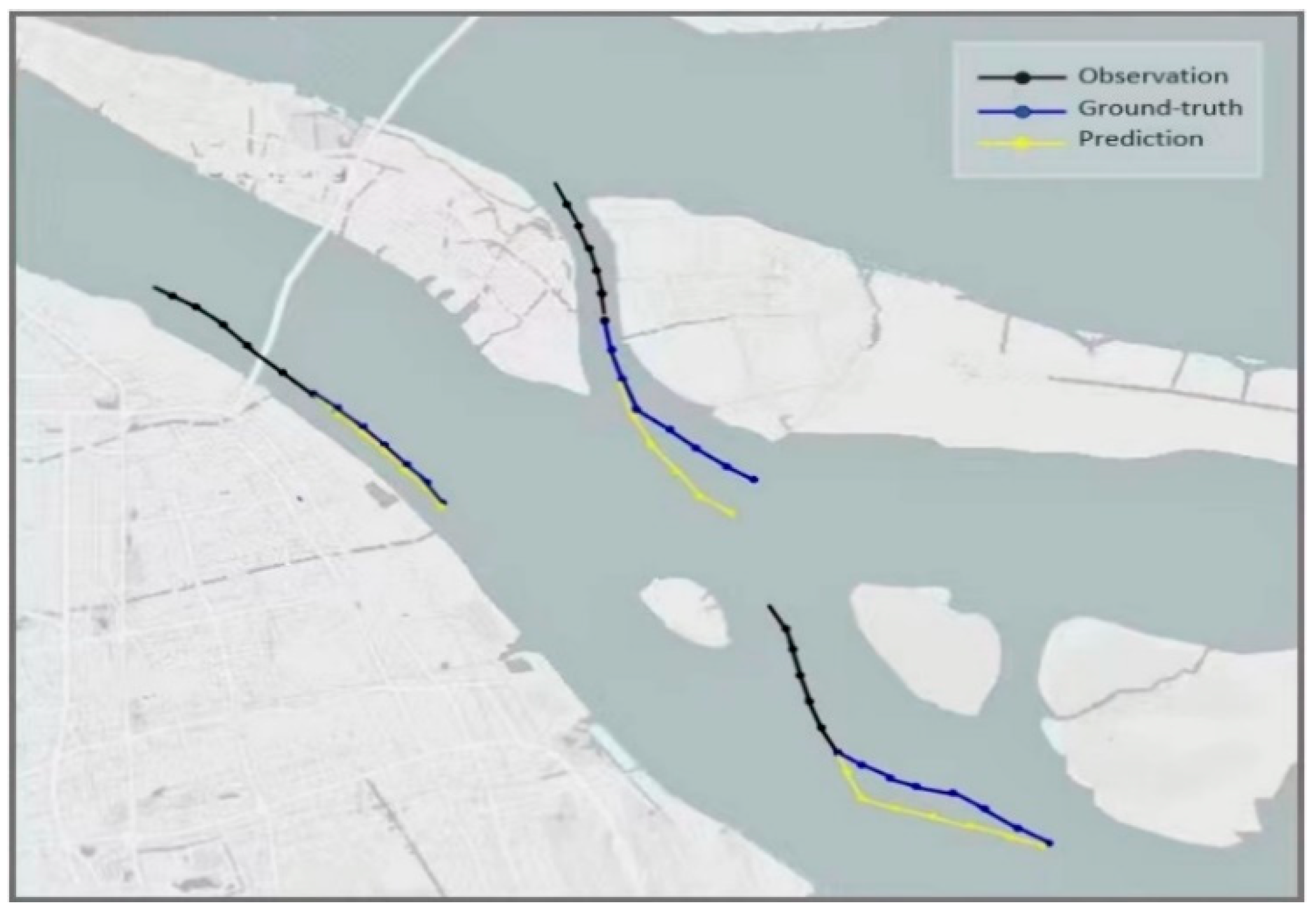
Figure 1. Selected trajectories from the dataset. Previously observed trajectories are marked in black. Ground-truth and predicted trajectories are marked as blue and yellow, respectively.
Jmse 10 01529 g001
Figure 2. Diagram of LSTM.
Jmse 10 01529 g002
Figure 3. Transformer model architecture.
Jmse 10 01529 g003
Figure 4. LSTNet architecture.
Jmse 10 01529 g004
Figure 5. Raw data distribution over time: (a) latitude (degree); (b) longitude (degree).
Jmse 10 01529 g005
Figure 6. Training and validation loss.
Jmse 10 01529 g006
Figure 7. Comparison of different models in a straight-line navigation state: (a) LSTM model, (b) LSTNet model, (c) GRU model (d) CNN model, (e) Transformer model.
Jmse 10 01529 g007aJmse 10 01529 g007b
Figure 8. Comparison of different models in waypoint navigation state: (a) Transformer model, (b) LSTNet model, (c) GRU model, (d) CNN model, (e) LSTM model.
Jmse 10 01529 g008aJmse 10 01529 g008b
Figure 9. Number of trainable parameters.
Jmse 10 01529 g009
Figure 10. Prediction performance of LSTM and CNN model.
Jmse 10 01529 g010
Table 1. LSTM configuration.
NameValue
Batches32
OptimizerAdam
Epochs160
Loss FunctionMSE
ActivationReLU
Table 2. Parameter settings for different models.
ModelLearning RateInput LayerHidden LayerBatch SizeActivation
GRU0.0011610032ReLU
LSTNet0.0011610020ReLU
Transformer0.0011610020ReLU
LSTM0.0011610032ReLU
CNN0.0011610032ReLU
Table 3. Prediction error comparison of different models.
ModelsRMSEMAE
Straight-line navigationLSTNet0.02100.0135
Transformer0.02380.0185
LSTM0.02630.0216
CNN0.02700.0219
GRU0.05360.0480
Waypoint navigationLSTNet0.03890.0310
Transformer0.04260.0384
LSTM0.05190.0475
CNN0.05360.0441
GRU0.07340.0677
Table 4. Prediction error comparison with variable input and output size.
Models (∆ l − 10)RMSE (∆ h + 4)MAE (∆ h + 4)
Straight-line navigationLSTNet0.02180.0133
Transformer0.02440.0190
LSTM0.02800.0231
CNN0.02830.0232
GRU0.05630.0503
Waypoint navigationLSTNet0.04580.0399
Transformer0.04890.0438
LSTM0.06140.0549
CNN0.06350.0586
GRU0.08410.0778
Table 5. RMSE comparison of both models.
LSTMCNN
East China Sea0.02380.0.265
Publisher’s Note: MDPI stays neutral with regard to jurisdictional claims in published maps and institutional affiliations.