Dominant Frequency Extraction for Operational Underwater Sound of Offshore Wind Turbines Using Adaptive Stochastic Resonance

Abstract

Underwater sound generated by the rapidly increasing offshore wind farms worldwide greatly affects the underwater soundscape and may cause long-term cumulative effects on sound-sensitive marine organisms. However, its analysis and impact assessment are heavily interfered with by underwater ambient noise. In this study, an adaptive stochastic resonance method is proposed to extract the dominant frequency of wind turbine operational sound when heavy noise is present. In particular, a time–frequency–amplitude fusion index was proposed to guide the parameter tuning of an adaptive stochastic resonance system, and an equilibrium optimizer based on the physical dynamic source–sink principle was adopted to optimize the parameter-tuning process. The results from the simulation and field data showed that the dominant frequency of operational sound was extracted adaptively. For field data with wind speeds of 4.13–6.15 m/s (at 90 m hub height), the extracted dominant frequency varied with wind speed between 90 and 107 Hz, and it was highly correlated with the wind turbine rotor speed monitored synchronously in the air, with a correlation coefficient of 0.985. Compared to other existing methods, our method has a higher output signal-to-noise ratio and a shorter running time.

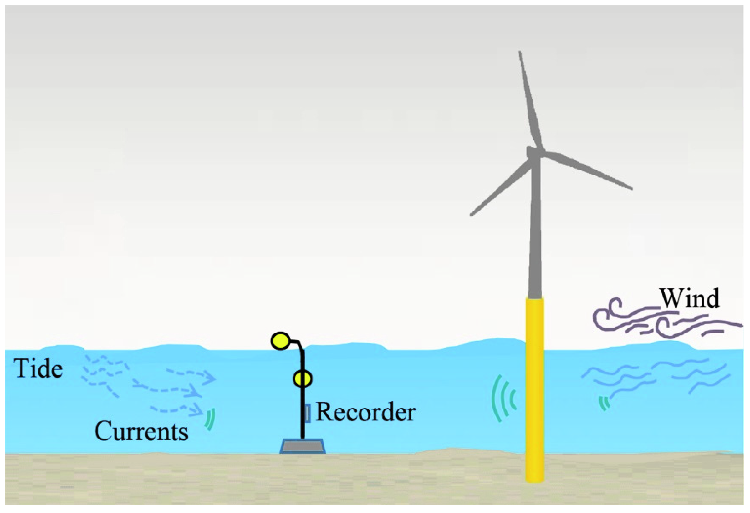
1. Introduction

As the next generation of clean energy, offshore wind power has entered a period of rapid development. In 2021, the total power capacity of installed offshore wind farms all over the world had increased from 5334 MW in 2011 to 55,678 MW [1]. While offshore wind turbines bring us benefits, they continue to radiate noise into the air and water during their operation period of 20–30 years. There are two main sources of wind turbine noise: aerodynamic noise and mechanical noise [2,3,4,5]. Aerodynamic noise is the main contributor to in-air noise [3,4], and due to the large characteristic impedance difference between water and air, it is almost completely reflected from the water surface and contributes less to the underwater noise level [5,6]. Underwater noise from operating wind turbines is mainly generated by mechanical vibrations of the gearbox and generator coupled into water after transmission from the nacelle to the tower and foundation [5,6,7,8]. With the increasing number and individual capacity of offshore wind turbines worldwide, underwater noise from offshore wind turbines has long-term and widespread effects on the underwater soundscape.

Sound is the sensory cue for marine animals, from invertebrates to great whales, and it is used to interpret and explore the ocean environment and to interact within and among species [9]. Underwater noise from operating wind turbines may have cumulative impacts on these sound-sensitive marine animals [10,11], such as masking acoustic communication, interfering with foraging and spawning, and triggering physiological responses [9,12,13,14]. It should be mentioned that underwater sound consists of sound pressure variations and particle vibration [15], and they are both important to fish [16,17,18]. This study mainly focuses on the sound pressure of underwater noise from operating wind turbines (hereafter referred to as the “operational signal” to distinguish it from underwater ambient noise).

The operational signal is usually described as a continuous, low-intensity sound with one or more tonal components below 1 kHz [5,6,7,8,19]. To systematically and scientifically analyze the operational signal and evaluate the long-term effects, a deep understand of its sound characteristics (both frequency and amplitude characteristics) is required. Since the frequency characteristics of operational signals from different types of wind turbines are different [20], and marine organisms have different sensitivities to different frequencies [9], the study of the frequency characteristics of operational signals is crucial. Previous studies have mainly used hydrophones and self-contained acoustic recorders to measure it. However, the operational signal can be easily disturbed by underwater ambient noise when the winds, tides, and ocean currents are strong (Figure 1), posing difficulties for measurement and analysis [7]. Therefore, this study focuses on extracting and analyzing the frequency characteristics of operational signals, which helps to comprehensively understand the operational signals under different sea states, and to provide a basis for environmental impact assessment, bioacoustic protection, and noise reduction design of future large-capacity wind turbines.

Unfortunately, traditional weak signal extraction techniques are not effective in extracting wind turbine operational signals. Traditional weak signal extraction methods, such as digital filter, matched filtering [21], discrete wavelet transform [22], and empirical mode decomposition [23], all consider noise as an interference and attempt to suppress noise to achieve the purpose of signal extraction. However, when the operational signal is disturbed by underwater ambient noise, the low signal-to-noise ratio (SNR) creates many limitations for these methods. For example, digital filter can effectively filter out the noise outside the passband but cannot remove the in-band noise. Moreover, the cut-off frequencies of the passband are difficult to choose accurately, especially when the desired signal is disturbed by noise and the dominant frequency of the signal varies with time. In this case, a mismatched setting of cut-off frequencies may lead to over-filtering or under-filtering of the data. Another popular method is matched filtering. However, the premise of using matched filtering method is that the source signature is known, which cannot be applied directly.

Unlike traditional methods, stochastic resonance (SR) views noise as a beneficial object, and it refers to the phenomenon when a weak periodic signal induces a nonlinear system to enhance periodic output with the assistance of noise under certain conditions [24,25]. By adjusting the parameters of an SR system, the optimal SR output can be realized to achieve weak signal extraction. Currently, the SR method has demonstrated great potential in weak signal extraction and has been applied in the underwater acoustic field, such as for underwater acoustic communication [26] and passive sonar detection [27].

Nevertheless, there are still some issues to be solved for using SR to extracting operational signals. On one hand, underwater ambient noise is often a mixture of noises from various sound sources, such as ocean turbulence, wind, biological activities, and traffic activities, which can be extremely complex. The noise can change with time, geographic location, and depth, and the dynamic range of noise levels is wide [28,29], making the suppression of underwater ambient noise difficult. On the other hand, the time–frequency characteristics of operational signals are related to many factors, such as turbine size [10,11], wind speed [7,8], and water depth [6]. In other words, the frequency characteristics of the operational signal of one wind turbine can be very different from others and can change over time. This complexity also makes the extraction of operational signals challenging.

To address these issues, this study proposes an adaptive stochastic resonance (ASR) method based on a time–frequency–amplitude fusion index (TFAI) and an equilibrium optimizer (EO) named TFAI-EO-ASR to extract operational signals under complex ambient noise. Under the guidance of TFAI, the TFAI-EO-ASR method adaptively tunes the system parameters to match the signal and noise through the EO to obtain the optimal ASR output and extract the dominant frequency. The novelty of this study is to propose the TFAI-EO-ASR method to overcome the interference of strong underwater ambient noise and to extract the dominant frequencies of operational signals adaptively under the condition of large dynamic changes in noise level. Secondly, a TFAI is constructed by fusing smoothness, peak SNR, and piecewise mean value through support vector regression, which effectively quantifies the system response and improves the extraction ability of the TFAI-EO-ASR method. Thirdly, an EO based on the physical dynamic source–sink principle is introduced as the optimization algorithm of the TFAI-EO-ASR method, which jointly optimizes the system parameters and improves the efficiency. Finally, the effectiveness and reliability of the TFAI-EO-ASR method are verified through a simulation and field measurement data obtained through simultaneous monitoring above and below the water during the operation period of an offshore wind farm. It should be noted that this study mainly focuses on extracting the frequency of operational underwater sound. The extraction of pressure amplitude, which requires further investigation on the nonlinear amplification effect of the ASR system, will be explored in our future study.

2. Materials and Methods

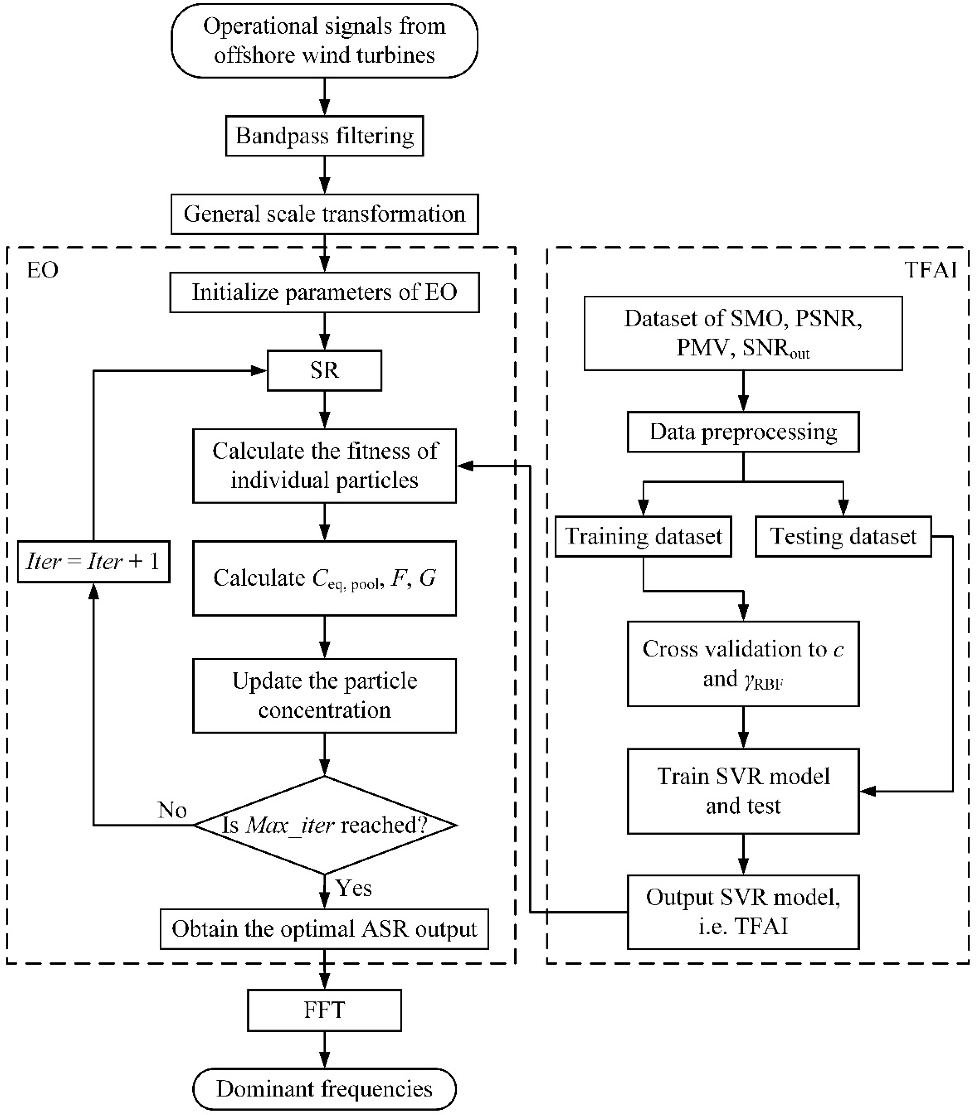
2.1. Adaptive Stochastic Resonance

Stochastic resonance is a method that utilizes noise energy to enhance weak periodic signals. It was first discovered and proposed by Benzi et al [24] in 1981 when explaining the cyclic recurrence of ice ages. After that, SR was also found in physical systems, such as Schmitt trigger circuits [30] and ring lasers [31]. With the development of the stochastic resonance theory, it has been applied in many fields, such as rotating machinery fault diagnosis [32], and optical image processing [33].

Stochastic resonance describes the phenomenon when a Brownian particle periodically transitions between potential wells at a speed of signal frequency under the cooperation of periodic signal and noise, thereby converting noise energy into signal energy [24,25]. The equation of motion of a unit-mass Brownian particle can be expressed as:

$$\frac{d^{2}x(t)}{d{t}^2}+\gamma \frac{dx(t)}{dt}-ax(t)+b{x}^3(t)=S(t)+N(t),$$

(1)

where a and b denote the potential parameters, γ is the damping factor, and $x(t)$ is the system output. $S(t)=A\sin (2\pi ft)$ is the periodic signal with amplitude A and frequency f. $N(t)=\sqrt{2D}\xi (t)$ is the noise term, D is the noise intensity, and $\xi (t)$ is the additive Gaussian white noise with zero mean and unit variance. When the signal, noise, and nonlinear system are properly matched, a Brownian particle experiences a strong periodic transition and converts part of the noise energy into the signal. Classical SR explained by adiabatic approximation theory can only be used to process signals with small parameters (i.e., $f\ll 1\mathrm{Hz}$, $A\ll 1$, $D\ll 1$) [34]. To apply classical SR to operational signals, a general scale transformation [35] is introduced:

$$x(t)=z(\tau ),\tau =mt,$$

(2)

where m is the scale coefficient. Equation (2) is substituted into Equation (1) to obtain:

$$\frac{d^{2}z}{d{\tau }^2}+{\gamma }_1\frac{dz}{d\tau }-a_{1}z+b_1{z}^3=A_1\sin (2\pi f_1\tau )+\sqrt{2D_{1}m}\xi (\tau ),$$

(3)

where $a_1=a/m^2$, $b_1=b/m^2$, ${\gamma }_1=\gamma /m$, $f_1=f/m$, $A_1=A/m^2$, and $\sqrt{D_1}=\sqrt{D}/m^2$. After rescaling, the signal frequency f₁ becomes 1/m times the original frequency f, and the signal amplitude becomes 1/m² times the original amplitude. By setting an appropriate m, the operational signal can meet the requirements of classical SR.

To further account for the temporal variability in the operational signal and underwater ambient noise, an adaptive stochastic resonance (ASR) method was used in this study. ASR refers to the adaptive adjustment of system parameters through an appropriate measurement index and an optimization algorithm to match the weak signal, noise, and nonlinear system to obtain the optimal output. The measurement index is used to quantify the SR system response and serve as the fitness of the optimization algorithm, while the optimization algorithm adjusts the system parameters under the guidance of the measurement index. When the system input–output SNR improvement (SNRI) is used as the measurement index, its relationship with a₁, b₁, and γ₁ is shown in Figure 2. Here, the signal amplitude is A = 0.1, the frequency is f = 100 Hz, the noise intensity is D = 10, and the scale coefficient is m = 2000. It can be seen that the SNRI varied with a₁, b₁, and γ₁. Then, the optimal SR output could be obtained by adjusting the system parameters to maximize the SNRI through ASR.

2.2. Time–Frequency–Amplitude Fusion Index

The measurement index of an ASR is a quantitative parameter that measures the performance of SR, which plays a crucial role in guiding the selection of system parameters. In most prior studies of ASR, SNR is usually used as the measurement index [27]. However, in this study, the operational signal was often disturbed by the underwater ambient noise, and the signal frequency could not be directly estimated, so SNR was not applicable. For a problem where the signal frequency is unknown, new measurement indices, such as weighted power spectrum kurtosis [36] and weighted spectral peak SNR (WPSNR) [37], have been proposed. These measurement indices are constructed by combining multiple basic indices, such as power spectrum kurtosis and correlation coefficient via multiplication and division, and have been successfully applied in the fault diagnosis of mechanical rotating parts. However, the simple multiplication and division method cannot well-fuse the advantages of each basic index, and it is easy to extract the wrong frequency when noise is strong. For this reason, Zhou et al. used a back propagation neural network to effectively fuse six basic indices into a new synthetic quantitative index [38]. However, too many basic indices were selected, and the setting of the neural network’s target value had a great influence on the performance of the synthetic quantitative index. For the extraction of operational signals under complex ambient noise, this study fused three basic indices from the time domain, frequency domain, and amplitude domain into a TFAI through support vector regression and took the results as the measurement index of the ASR method.

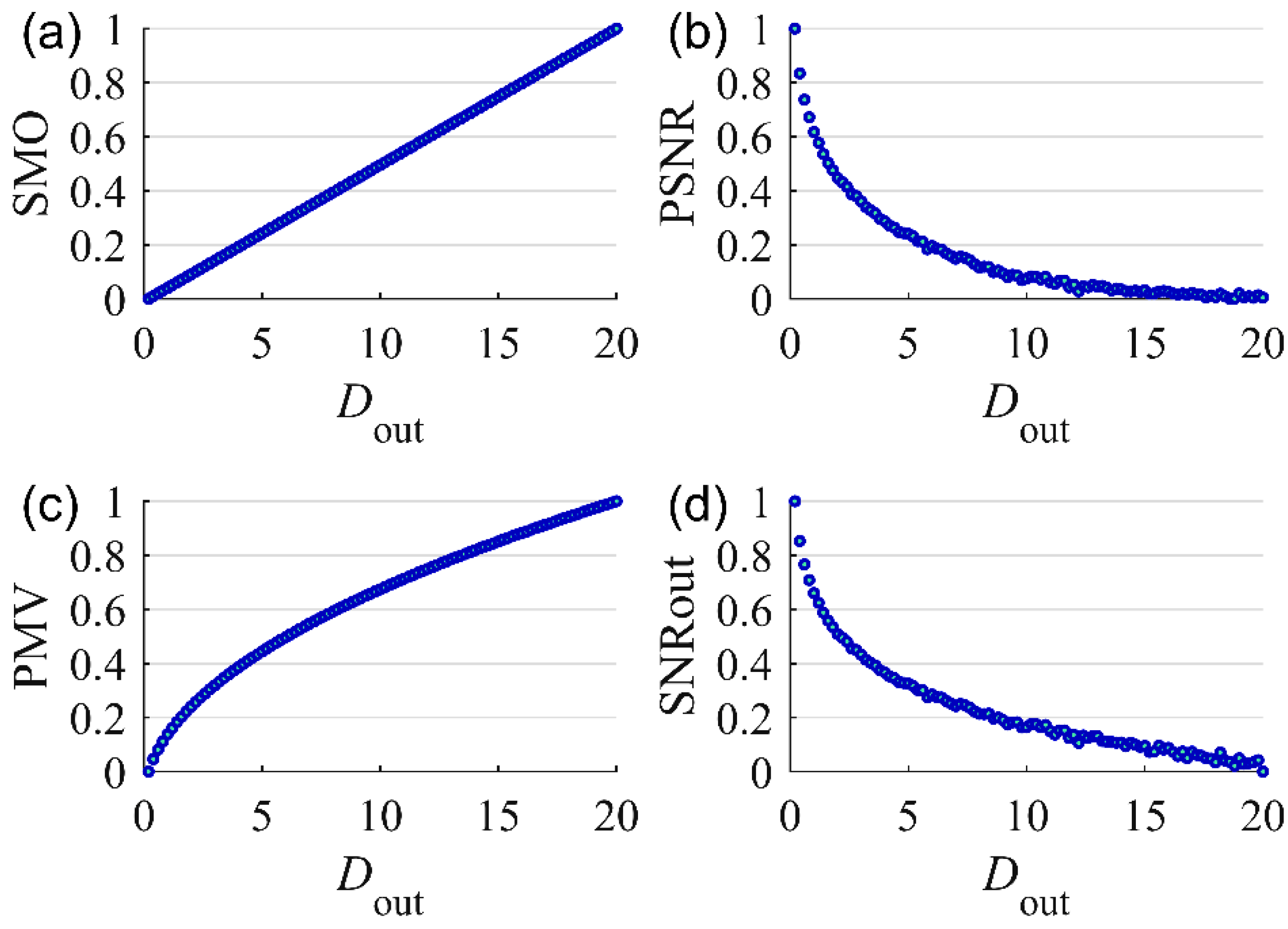
2.2.1. Selection of Basic Indices for Filtering Quality Evaluation

Basic indices that are frequently used to evaluate filtering quality include power spectrum kurtosis, correlation coefficient, root mean square error, etc. However, the performances of these indices may degrade significantly when the signal characteristics are completely submerged under strong noise. For this reason, these indices were abandoned in this study, and we adopted three other indices (i.e., smoothness, peak SNR, and piecewise mean value) selected from the time domain, frequency domain, and amplitude domain.

(1) Smoothness (SMO) is the ratio of the sum of squared sequential differences in the output signal to such a sum in the input signal, which can be expressed as:

$$\mathrm{SMO}=\frac{{\displaystyle \sum _{n=1}^{N-1}{\left[x(n+1)-x(n)\right]}^2}}{{\displaystyle \sum _{n=1}^{N-1}{\left[y(n+1)-y(n)\right]}^2}},$$

(4)

where x(n) is the output signal, and y(n) is the input signal. The smaller the SMO, the better the denoising effect.

(2) Peak SNR (PSNR) is the ratio of the maximum signal power to the noise power, which can be expressed as:

$$\mathrm{PSNR}=10\log \left(\frac{X_{(n_0)}^2}{{\displaystyle \sum _{n=1}^{N/2}{X}_{(n)}^2-X_{(n_0)}^2}}\right),$$

(5)

where $X_{(n)}$ is the power spectrum of x(n), $X_{(n_0)}$ is the power spectrum at peak frequency, and N is the number of signal points. A larger PSNR suggests a better denoising effect of an SR system.

(3) Piecewise mean value (PMV) describes the difference in the mean value of the amplitude of each segmented signal [39]. To ensure that the PMV changes monotonically with noise intensity, it is deformed as follows:

$$\mathrm{PMV}=\sqrt{\frac{1}{l_0-1}{\displaystyle \sum _{l=1}^{l_0-1}{(x_l-x_{\mathrm{mean}})}^2}},$$

(6)

where l₀ is the number of zero-crossing points, $x_l$ is the mean amplitude of the lth signal segment, and $x_{\mathrm{mean}}$ is the mean amplitude of the entire signal. The smaller the PMV, the better the output of the SR system.

2.2.2. Fusion of Multiple Basic Indices

The fusion of multiple basic indices was realized through support vector regression (SVR). It is a regression model based on the principle of structural risk minimization, which can find the best compromise between model complexity and empirical error according to limited sample information and has a good generalization ability [40].

For the dataset $\{(P_i,Q_i),i=1,2,\cdots ,{\mathrm{n}}_s\}$, $P_{\mathrm{i}}={\left[{\mathrm{SMO}}^i,{\mathrm{PSNR}}^i,{\mathrm{PMV}}^i\right]}^T$ is the input vector with three-dimensional eigenvalues, $Q_{\mathrm{i}}={\left[{\mathrm{SNR}}_{\mathrm{out}}^i\right]}^T$ is the one-dimensional output vector, and n_s is the number of samples. After mapping the input vector to the high-dimensional space through a mapping function $\mathsf{\Psi }(P)$, an SVR model is constructed as follows:

$$F(P)=w\mathsf{\Psi }(P)+d,$$

(7)

where w is the weight vector, d is the intercept, and F(P) is the TFAI.

According to the principle of structural risk minimization, the optimization problem is formulated as:

$$\{\begin{array}{l}\min \frac{1}{2}{\Vert w\Vert }^2+c{\displaystyle \sum _{i=1}^{n_s}({\delta }_i+{\delta }_i^{’})}\\ subjectto\{\begin{array}{l}{Q}_i-(w\mathsf{\Psi }(P_i)+d)\le \epsilon +{\delta }_i\\ w\mathsf{\Psi }(P_i)+d-Q_i\le \epsilon +{\delta }_{\mathrm{i}}^{’}\\ {\delta }_i\ge 0,{\delta }_i^{’}\ge 0\end{array}\end{array},$$

(8)

where ${\delta }_i$ and ${\delta }_i^{’}$ are relaxing factors, and $\epsilon$ is the error term. The SVR model allows a maximum error of $\epsilon$ between the predicted value and the target value; otherwise, a penalty is applied. c is the penalty factor, which balances the prediction accuracy and model complexity. The larger the c, the less tolerance for errors. In addition, a kernel function is used in the SVR model to map samples to a high-dimensional feature space. Typical kernel functions include linear, polynomial, and Gaussian functions, as well as radial basis function (RBF). Among them, the RBF is adopted by most scholars due to its good universality and accuracy. Therefore, RBF was also used here, and the definition is as follows:

$$K_{\mathrm{RBF}}(P_i,P_j)=\exp (-{\gamma }_{\mathrm{RBF}}{\Vert P_i-P_j\Vert }^2),$$

(9)

where ${\gamma }_{\mathrm{RBF}}$ is the kernel parameter of RBF.

By constructing a Lagrangian dual function to solve the optimization problem of Equation (8), the TFAI can be obtained. In this study, the index fusion was implemented in MATLAB R2018b (Mathworks Inc., Natick, MA, USA) using the LIBSVM [41] library. The specific steps were as follows.

(1)

Dataset generation. The periodic signal was superimposed with high-intensity ($D=D_{\mathrm{m}}$) Gaussian white noise to generate a system input. After that, the same periodic signal was superimposed with Gaussian white noise of different intensities ($D\in (0,D_{\mathrm{m}}]$) to generate multiple system outputs. For each input–output pair, the corresponding SMO, PSNR, and PMV were calculated as the eigenvalues of the samples, and the $SN{R}_{\mathrm{out}}$ of the target signal was taken as the target value, thus forming a dataset.

(2)

Data preprocessing. To prevent an eigenvalue from being too large or too small, resulting in an unbalanced effect in the regression, the dataset needed to be normalized. The normalization process was as follows:

$$P’=\frac{P-P_{\min }}{P_{\max }-P_{\min }},$$

(10)

where $P_{\max }$ and $P_{\min }$ are the maximum and minimum values of each group of eigenvalue data, respectively; $P$ is the original data; and $P’$ is the normalized data with a range of [0, 1]. Then, 80% of the total data were randomly selected as the training dataset, and the remaining 20% were used as the testing dataset.

(3)

Parameter settings. The RBF was selected as the kernel function of the SVR model, and the values of c and ${\gamma }_{\mathrm{RBF}}$ were determined using cross-validation and a grid search.

(4)

Training and testing. The training dataset was used to construct the SVR model and measure its accuracy, and the testing dataset was used to evaluate its generalization ability. Finally, the generated model was the TFAI.

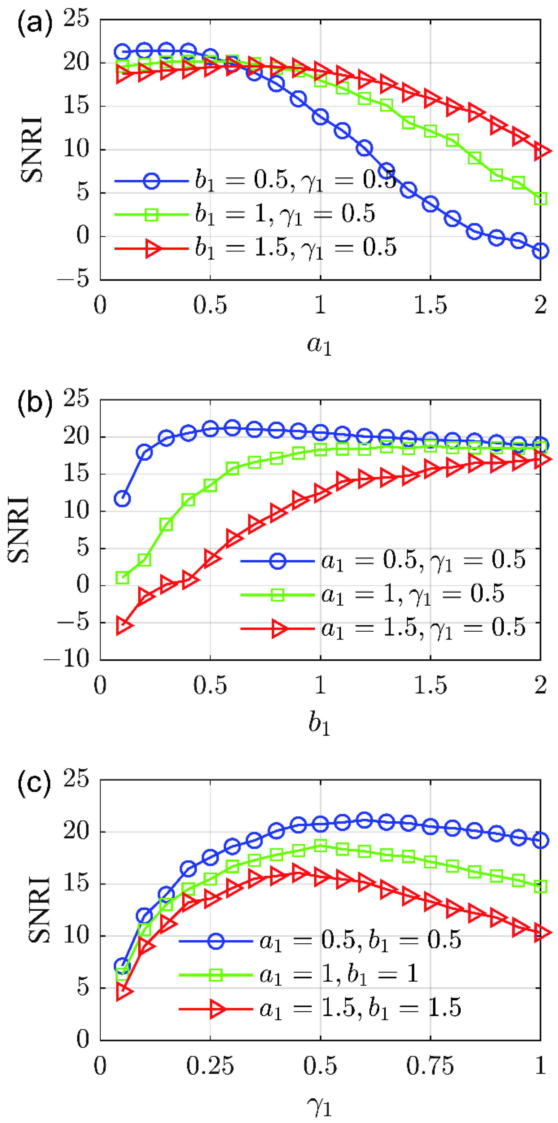
2.3. Equilibrium Optimizer

A traditional ASR method uses a grid search method to find system parameters, which is computationally intensive and inefficient. To find the optimal parameters more accurately and quickly, some swarm intelligence optimization algorithms have been applied to ASR, including the artificial fish swarm algorithm (AFSA) [36] and gray wolf optimizer [42]. Compared with these algorithms, an equilibrium optimizer (EO) has the strengths of simple calculation, strong optimization ability, and fast convergence speed. It is a new metaheuristic optimization algorithm based on controlled-volume mass balance models and proposed by Faramarzi et al. in 2020 [43]. The algorithm takes Equation (11) as the core of the framework to carry out iterative optimization:

$$C=C_{\mathrm{eq}}+(C_0-C_{\mathrm{eq}})F+G(1-F)/\lambda V,$$

(11)

where V and C are, respectively, the size and concentration of the volume, and $\lambda$ is a random vector between 0 and 1. F is the exponential term, and G is the generation rate inside the volume, both of which are important rules for concentration update and serve to balance the direct search and global search. $C_{\mathrm{eq}}$ represents the concentration at an equilibrium state, and it is randomly selected from the equilibrium pool. The equilibrium pool is composed of four solutions, $C_{\left(1\right)}$, $C_{\left(2\right)}$, $C_{\left(3\right)}$, $C_{\left(4\right)}$, with the best fitness at present and their average states. It can be expressed as:

$$C_{\mathrm{eq},\mathrm{pool}}=\{C_{\left(1\right)},C_{\left(2\right)},C_{\left(3\right)},C_{\left(4\right)},C_{\mathrm{eq}\left(\mathrm{ave}\right)}\}.$$

(12)

For the optimization of ASR system parameters, C represents the newly generated current solution, C₀ is the solution obtained from the previous iteration, and $C_{\mathrm{eq}}$ corresponds to the current optimal solution, which was implemented as follows.

(1)

Initialization. The range of ASR system parameters a₁, b₁, and γ₁, the number of particles, and the maximum iterative number Max_iter were set, and the initial concentration of individual particles was initialized.

(2)

Evaluation. SR was performed according to the particle concentration, and the TFAI was calculated as the fitness of individual particles.

(3)

Update. The equilibrium pool $C_{\mathrm{eq},\mathrm{pool}}$ was calculated, as well as the exponential term F and the generation rate G in turn, and the particle concentration was updated according to Equation (11).

(4)

Termination. It was judged whether the current iteration Iter reached Max_iter. If so, the particle concentration corresponding to the maximum fitness was saved, and the optimal ASR signal was output. Otherwise, Iter = Iter + 1, and steps (2) and (3) were repeated.

In this study, the TFAI-EO-ASR method took the TFAI as the measurement index and jointly optimized the system parameters a₁, b₁, and γ₁ via EO to obtain the optimal ASR output and extract the dominant frequencies of operational signals. The flowchart is shown in Figure 3.

3. Results

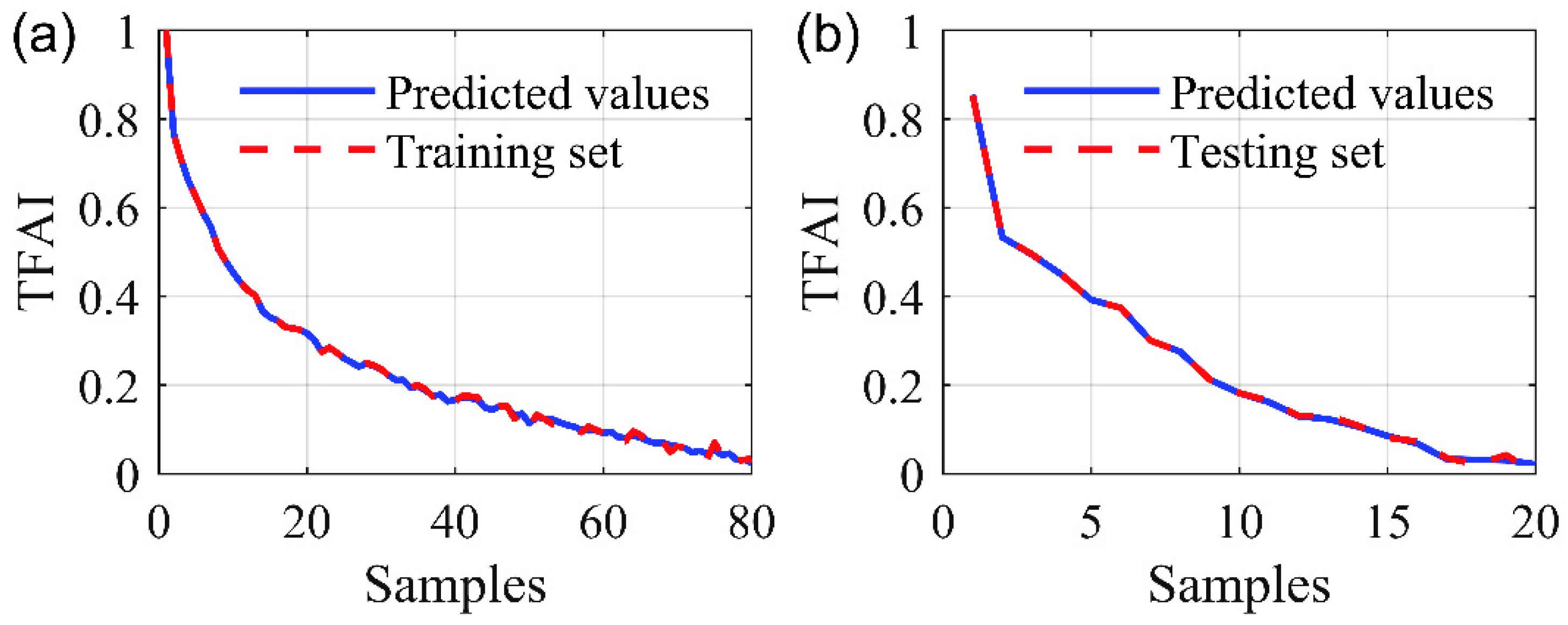
3.1. Analysis of TFAI

A periodic signal with a frequency f of 100 Hz and an amplitude A of 0.1 was used as an example to construct the TFAI. The other parameters were set as follows: the noise intensity of the system input D_in was 20, the noise intensity of the system output D_out varied from 0.2 to 20 with a variation step of 0.2, the sampling rate was 128 kHz, and the signal duration was 1 s. After calculation, a total of 100 samples were generated, and each sample was the average of 100 repeated calculations. The distribution of normalized samples with noise intensity D_out is showed in Figure 4. As seen in Figure 4, the SMO, PSNR, and PMV, similar to the SNR_out, changed monotonically with increasing D_out, indicating that these basic indices were able to describe the noise content of a signal from different aspects (i.e., time domain, frequency domain, and amplitude domain).

Then, the basic indices were fused with the SVR model to construct the TFAI. The training and testing results of the SVR model are shown in Figure 5. The penalty factor c and kernel parameter ${\gamma }_{\mathrm{RBF}}$ were automatically set to 67.6032 and 0.1238, respectively, using cross-validation and a grid search. It can be seen that the predicted values of SVR were close to the target values in both the training dataset and the testing dataset, and the squared correlation coefficients were greater than 0.99. This indicates that the generated TFAI (SVR model) effectively fused information in the time domain, frequency domain, and amplitude domain and had good accuracy and generalization ability.

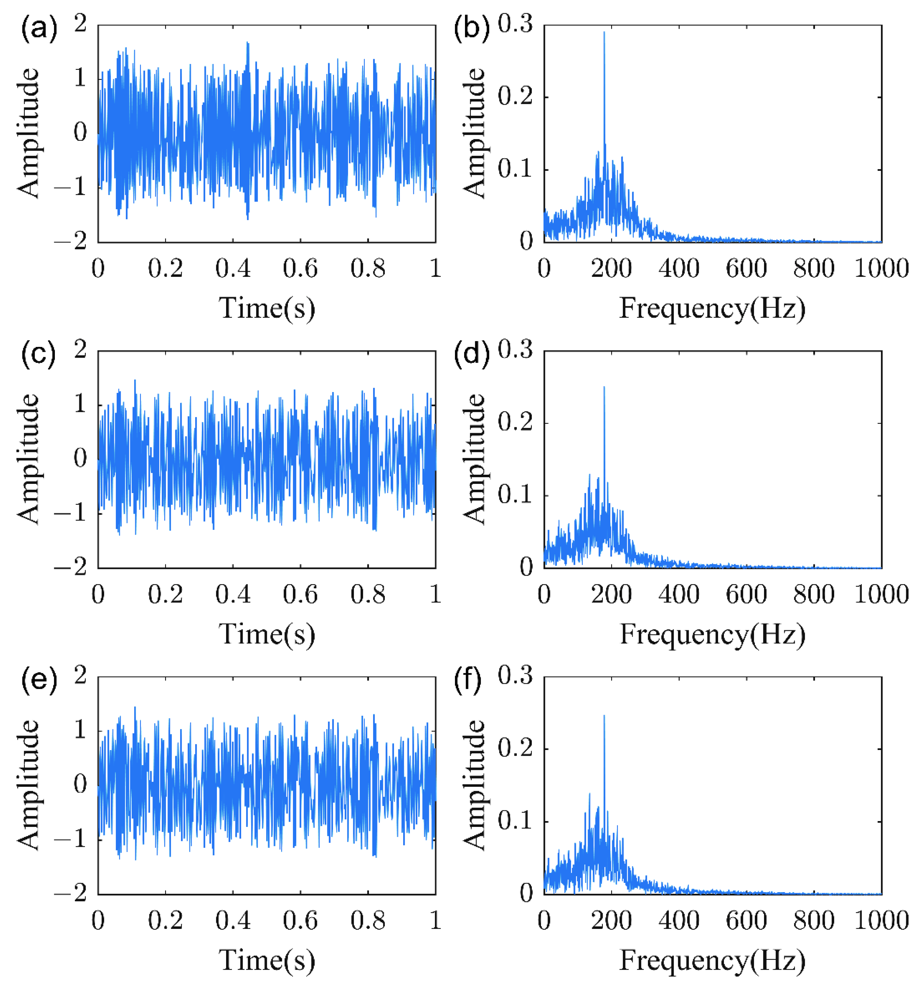
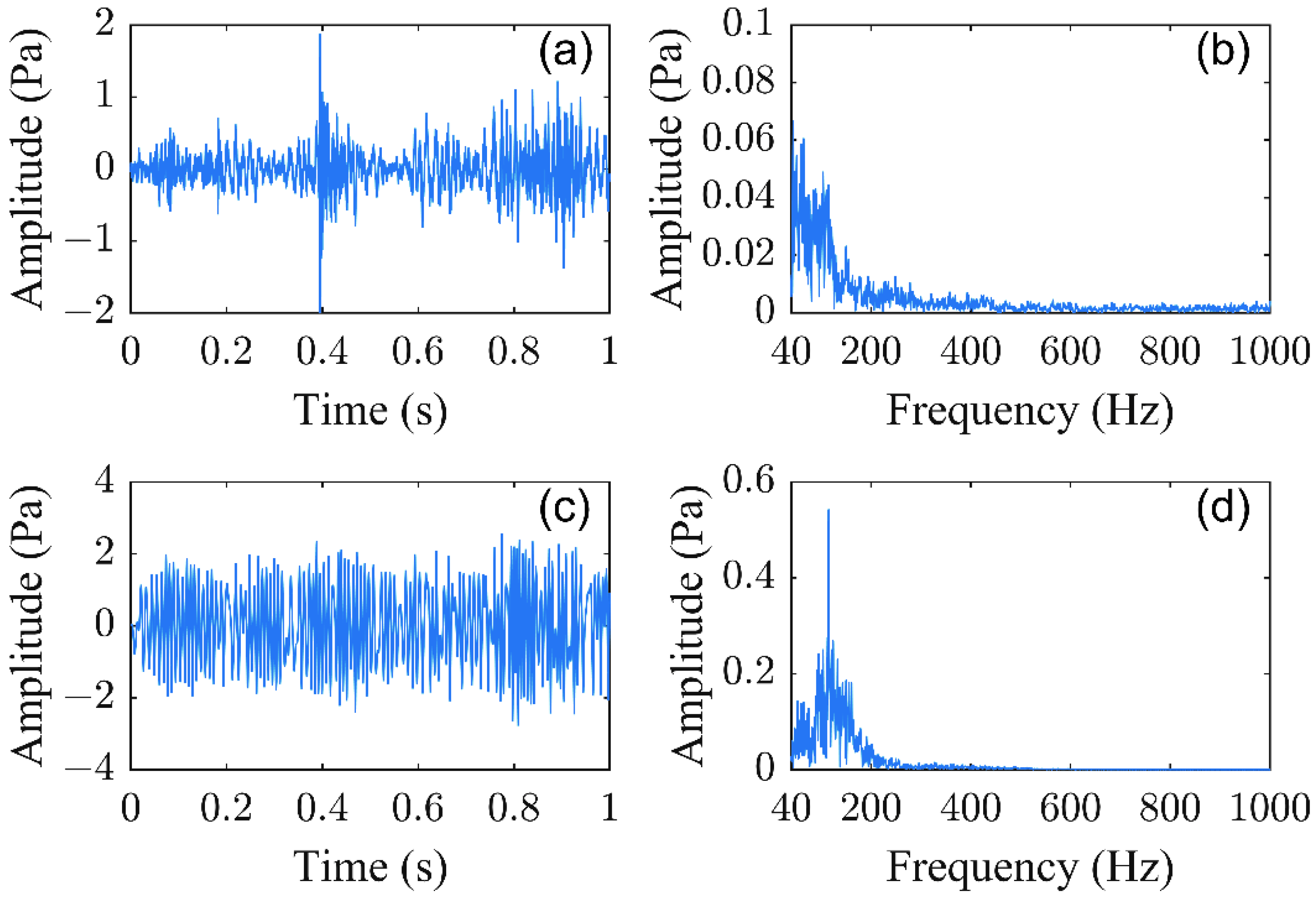
3.2. Verification with Simulation

To verify the effectiveness of the proposed method, a noisy signal was generated by superimposing a periodic signal and Gaussian white noise, and the proposed TFAI-EO-ASR method was used to extract the dominant frequency. According to Lindell’s field data from Utgrunden offshore wind farm, the operational signal was characterized by a line spectrum with a frequency of 178 Hz [6]. In addition, the spectrum of underwater ambient noise was approximately flat when the bandwidth of the analysis was narrow. Therefore, a periodic signal with a frequency of 178 Hz and an amplitude of 0.08 was taken as the target signal, and Gaussian white noise with an intensity of 8 was used as the underwater ambient noise. The sampling frequency was 128 kHz, and the duration was 1 s. After the periodic signal was superimposed with the noise, the waveform and spectrum of the noisy signal are shown in Figure 6a,b. It can be seen that the periodic signal was completely submerged by the noise, and there were no obvious characteristics in the spectrum. The input SNR was −22.8 dB (0–1 kHz). It should be noted that this noisy signal may be different from the actual situation, but the purpose here is not to mimic the actual signal, but to validate and gain an understanding of the detection performance of the ASR method in complex underwater acoustic environment.

In this simulation analysis, the scale coefficient m was 1000, the number of particles was 50, the maximum iterative number was 50, the range of a₁ and b₁ was (0, 2], and the range of γ₁ was (0, 1]. Figure 6c,d shows the waveform and spectrum of the TFAI-EO-ASR output signal respectively, and the corresponding optimal system parameters were $a_1=0.0067$, $b_1=1.2670$, and ${\gamma }_1=0.1094$. Compared with Figure 6a, the noise interference in Figure 6c was significantly reduced, and the target periodic signal was effectively extracted from the noise. From the spectrum of the TFAI-EO-ASR output (Figure 6d), it can be seen that there was a clear line spectrum at 178 Hz with the energy at other frequencies effectively suppressed, and therefore, the frequency of the target periodic signal could be easily determined as 178 Hz. At this time, the output SNR was −8.3 dB, which was 14.5 dB higher than the input SNR, indicating that the TFAI-EO-ASR method could effectively extract the frequency of the noisy signal.

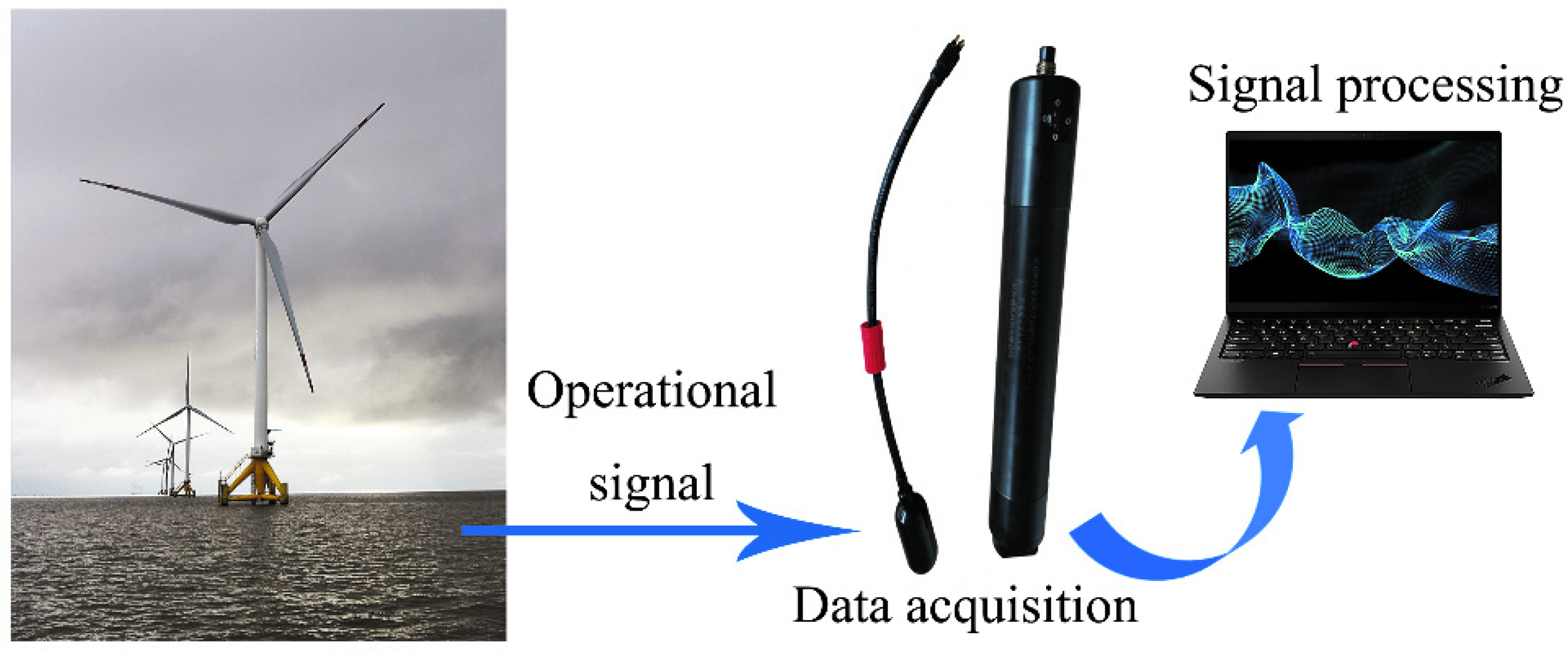
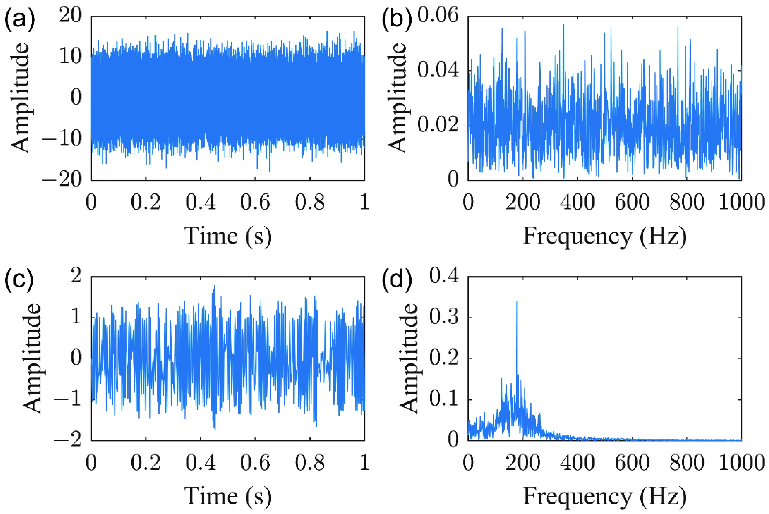
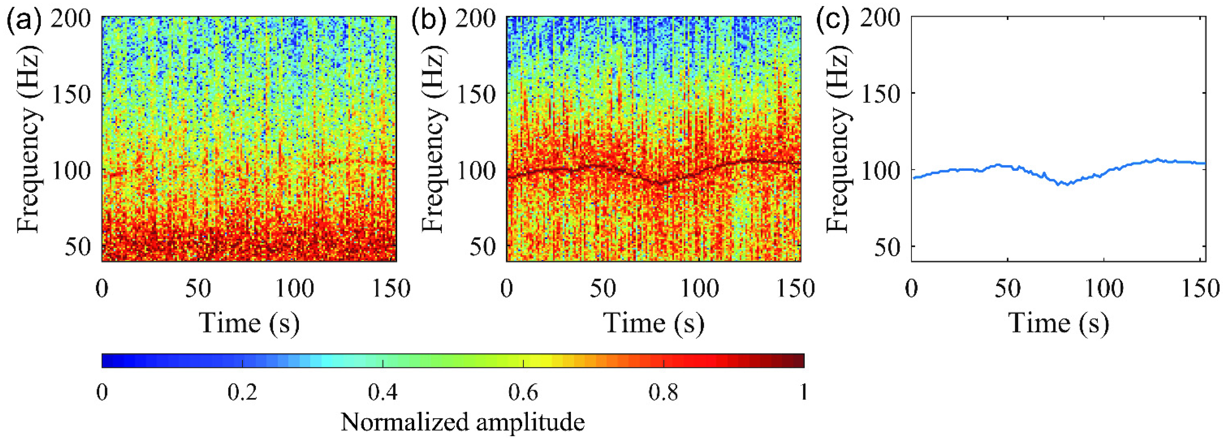
3.3. Verification with Field Data

The field measurement of operational signals was conducted at an offshore wind farm in Rudong waters, Jiangsu Province, China, on 20 June 2019. The measured wind turbine was of a doubly-fed asynchronous and variable speed type, with a rated power of 4.0 MW and a tripod foundation (Figure 7). The water depth in the wind farm area was about 8 m, and the seabed was relatively flat. The weather was cloudy during the monitoring period, and the wind speed at the hub (90 m) varied from 3.4 to 8.7 m/s. Operational signal data were collected using a self-contained LoPAS-L acoustic recorder (LoPAS-L, Hangzhou SonicInfo Technology Co., Ltd., Hangzhou, China), as shown in Figure 7. The LoPAS-L had an omnidirectional broadband hydrophone with a sensitivity of 234.4 μV/Pa and a resolution of 24 bits. Operational signals were recorded continuously at a sample rate of 128 kHz. The LoPAS-L was deployed at the middle layer of the water, approximately 15 m away from the tripod foundation. During the measurement, ship engines and other equipment that could generate sound were turned off.

The temporal waveform and frequency spectrum of the collected operational signal after band-pass filtering are shown in Figure 8a,b. Because the noise below 40 Hz was mainly caused by the vibration of equipment or the hydrophone due to tidal fluctuation rather than ambient noise or operational signals [8], frequencies below 40 Hz were not considered in this study. As seen from Figure 8a,b, the line spectrum of the operational signal was submerged in the ambient noise, and it was difficult to determine the dominant frequency of the operational signal directly. After processing with the TFAI-EO-ASR method, the waveform and spectrum of the output signal are shown in Figure 8c,d. Here the scale coefficient m was 1000, the particle number of the EO was 50, the maximum iterative number was 50, the range of a₁ and b₁ was (0, 2], and the range of γ₁ was (0, 1]. It can be easily found that the TFAI-EO-ASR output signal had a clear line spectrum at 115 Hz, while other noise components were significantly suppressed. Therefore, the dominant frequency of the collected operational signal could be easily determined as 115 Hz.

Figure 9a shows a time–frequency diagram of the collected operational signal with a duration of 153 s, which was obtained by the spectrogram function of MATLAB R2018b (Mathworks Inc., Natick, MA, USA) with normalized amplitude. The corresponding spectrogram parameters were set as follows: the window length is 1–s and the overlap rate is 0. During this period, the wind speed at the hub height (90 m) varied from 4.13 to 6.15 m/s. Due to the influences of tide and wind, there were many interferences in the time–frequency diagram, and the line spectrum characteristics were not clear. After being processed with the TFAI-EO-ASR method, a clear line spectrum appeared in the time–frequency diagram (Figure 9b), and its frequency fluctuated in the range of 90–107 Hz (Figure 9c). The parameter settings in Figure 9b were the same as those in Figure 9a. Results in Figure 9 indicates that the TFAI-EO-ASR method could effectively track and extract the dominant frequency of the operating signal under the dynamic change in the noise level.

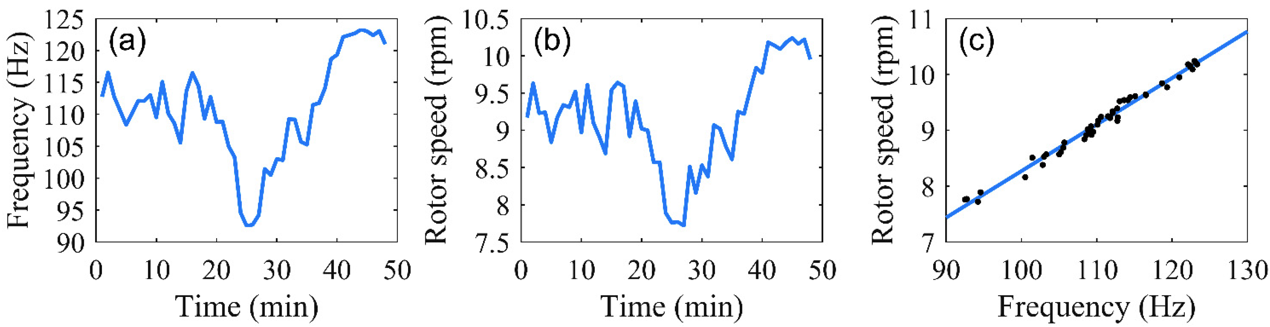
3.4. Comparison of Extracted Dominant Frequency and Wind Turbine Rotor Speed

To verify that the extracted frequency results of the TFAI-EO-ASR method truly reflected the dominant frequency of the operational signal, the extracted dominant frequencies were further analyzed with the wind turbine rotor speeds monitored synchronously in the air. The wind turbine rotor speed data were provided by a wind power company, and each piece of data was the average result of 1 min. Figure 10a shows the dominant frequencies extracted from the operational signals after TFAI-EO-ASR processing, and Figure 10b shows the variation curve of the rotor speed in the air during the same period. It can be seen that the dominant frequency and the rotor speed had almost the same variation tendency. If the two were linearly fitted (Figure 10c), the fitted correlation coefficient was as high as 0.985, indicating a strong correlation between the two. Such a similar variation tendency between the dominant frequency of the operational signal and the rotor speed in the air was also reported in a previous study in Pangerc’s field [8]. This further confirms that the frequencies extracted with the TFAI-EO-ASR method in this study were the dominant frequencies of the operational signals from an offshore wind farm. Therefore, the TFAI-EO-ASR method was reliable.

4. Discussion

An operational signal under complex ambient noise was extracted using an ASR method in this study. The key to the successful application of this method was to find appropriate system parameters that matched the signal, noise, and nonlinear system so that the optimal ASR output was achieved. In the proposed method, the system parameters were selected through an EO under the guidance of a TFAI so that they could have a great impact on the extraction results. To evaluate the performances of the TFAI and EO, other methods with other measurement indices (e.g., WPSNR) and optimization algorithms (e.g., AFSA) were compared. Among them, WPSNR is constructed by fusing the PSNR, spectral correlation coefficient, and zero-crossing point ratio, and was successfully applied in the ASR processing of rolling bearing fault diagnosis [37]. AFSA is a swarm intelligence optimization algorithm that imitates the foraging, swarming, and rear-ending behaviors of artificial fish and has the advantages of robustness, insensitivity to initial values, and ease of jumping out of the local extreme value and obtaining the global extreme [36]. In the comparison, different combinations of measurement indices and optimization algorithms for ASR were used, and the output SNR was adopted to evaluate the extraction performance, with the running time used to evaluate the extraction efficiency. To avoid the interference of other factors, the parameters of AFSA were set consistently with the EO, and the input signal was uniformly adopted as the noisy signal shown in Figure 6a,b. The computational environment of the method was MATLAB R2018b on a 64-bit Windows 10 operating system, and the computer hardware was Inter Core i5-4460 CPU with 16 GB memory.

The extraction results of different ASR methods are shown in Figure 11, and the corresponding operating parameters are shown in

Table 1. Parameters of adaptive stochastic resonance extraction.

Method	SNR/dB	Running Time/s
TFAI-EO-ASR	−8.3	251.9
TFAI-AFSA-ASR	−9.4	1183.0
WPSNR-EO-ASR	−9.7	235.9
WPSNR-AFSA-ASR	−9.8	935.4

. Comparing Figure 6, Figure 11, and Table 1, no matter which optimization algorithm was adopted, the results obtained by ASR methods with the TFAI as the measurement index had more prominent line spectrum characteristics, more complete suppression of the remaining noise components, and higher output SNRs, indicating that the TFAI had a better performance. In addition, no matter which measurement index was adopted, the running times required for the ASR methods with EO as the optimization algorithm were always less, at only one-quarter of that of AFSA, indicating that EO was simple, fast, and efficient. In general, compared with the ASR methods using WPSNR as the measurement index or AFSA as the optimization algorithm, the TFAI-EO-ASR method proposed in this study had certain superiority in extraction performance and efficiency.

The reliable extraction of the dominant frequencies of offshore wind turbine operational signals enabled by our proposed method could benefit a variety of studies related to environment, biology, and physics. For example, our results revealed that the dominant frequencies of operational signals varied in the range of 90–107 Hz under wind speeds of 4.13–6.15 m/s. By comparing the extracted dominant frequencies with the auditory threshold curve of a particular marine animal, one could assess whether a wind turbine operational signal is within the hearing range of this animal. Our results showed that the dominant frequency range greatly overlapped with the hearing thresholds of most fish (50–500 Hz) [18], suggesting that the operational signals of offshore wind turbines can be sensed by most fish. As the size and number of offshore wind turbines increase, the sound pressure levels of operational signals may also increase, leading to long-term cumulative effects on fish and posing a series of environmental concerns [10,11]. Our dominant frequency extraction method is helpful for the long-term monitoring of cumulative effects and the assessment of related environmental impacts. The extraction of frequencies contributes to the development of pressure amplitude extraction techniques for operational signals, which are important for the quantitative analysis of their cumulative effect. Our method can further help subsequent analyses of the relationship of operational signals with the physical marine environment (e.g., wind speed, wind direction, and flow velocity) and lay a theoretical foundation for acoustic environmental impact assessment and the low-noise design of future large-capacity wind turbines. In addition, the dominant frequency had a consistent trend with the rotor speed in the air, as operational signals originate from the mechanical rotating parts of wind turbines [8]. By extracting the dominant frequency of the operational signal through TFAI-EO-ASR, the rotor speeds of offshore wind turbines can be derived, providing a non-contact method for rotor speed monitoring and overspeed protection. Beyond that, the TFAI-EO-ASR method could also be applied to other fields related to the detection of weak signals in strong underwater ambient noise, such as underwater acoustic communication.

5. Conclusions

In this study, the TFAI-EO-ASR method was proposed for the problem of operational signals from offshore wind farms being weak, easily disturbed by underwater ambient noise, and difficult to analyze. Under the guidance of the TFAI, the TFAI-EO-ASR method adaptively tuned the system parameters with an EO to realize the extraction of the dominant frequency of the operational signal. The TFAI was constructed by fusing the SMO, PSNR, and PMV through SVR and effectively quantified the system output response and solved the problem of unknown frequency of the operational signal under heavy ambient noise. The EO jointly optimized multiple system parameters according to the principle of physical dynamic source–sink to improve the efficiency of signal extraction. The analysis results of the simulation and field data showed that the output SNR of the signal to be measured was significantly improved, and the line spectrum was clearer after processing with the TFAI-EO-ASR method, which indicated that the method could effectively extract the dominant frequency of the operational signal. Based on this, a comparison between the extracted frequencies of operational underwater signals and the wind turbine rotor speed synchronously monitored in the air showed that the two parameters had a consistent trend, and the fitting correlation coefficient was as high as 0.985, which further proved the reliability of the TFAI-EO-ASR method. Moreover, a higher output of SNR and a shorter running time of the proposed method were shown by comparing ASR methods using different measurement indices (e.g., TFAI, WPSNR) and optimization algorithms (e.g., EO, AFSA).

In future work, we plan to combine other methods, such as the chaotic critical state method, to extract the amplitude information of operational underwater sound from offshore wind turbines. In addition, we intend to extend our method to study particle motion and its impact on fish.

References

- IRENA; GEC. Renewable Capacity Statistics 2022; International Renewable Energy Agency: Abu Dhabi, United Arab Emirates, 2022. [Google Scholar]
- Leung, D.Y.C.; Yang, Y. Wind energy development and its environmental impact: A review. Renew. Sustain. Energy Rev. 2012, 16, 1031–1039. [Google Scholar] [CrossRef]
- Jianu, O.; Rosen, M.A.; Naterer, G. Noise pollution prevention in wind turbines: Status and recent advances. Sustainability 2012, 4, 1104–1117. [Google Scholar] [CrossRef] [Green Version]
- Tabassum, A.; Premalatha, M.; Abbasi, T.; Abbasi, S.A. Wind energy: Increasing deployment, rising environmental concerns. Renew. Sustain. Energy Rev. 2014, 31, 270–288. [Google Scholar] [CrossRef]
- Tougaard, J.; Henriksen, O.D.; Miller, L.A. Underwater noise from three types of offshore wind turbines: Estimation of impact zones for harbor porpoises and harbor seals. J. Acoust. Soc. Am. 2009, 125, 3766–3773. [Google Scholar] [CrossRef] [PubMed] [Green Version]
- Lindell, H. Utgrunden Off-Shore Wind Farm-Measurements of Underwater Noise; Ingemansson Technology AB: Gothenburg, Sweden, 2003. [Google Scholar]
- Yang, C.M.; Liu, Z.W.; Lü, L.G.; Yang, G.B.; Huang, L.F.; Jiang, Y. Observation and comparison of tower vibration and underwater noise from offshore operational wind turbines in the East China Sea Bridge of Shanghai. J. Acoust. Soc. Am. 2018, 144, EL522–EL527. [Google Scholar] [CrossRef] [PubMed] [Green Version]
- Pangerc, T.; Theobald, P.D.; Wang, L.S.; Robinson, S.P.; Lepper, P.A. Measurement and characterisation of radiated underwater sound from a 3.6 MW monopile wind turbine. J. Acoust. Soc. Am. 2016, 140, 2913–2922. [Google Scholar] [CrossRef] [PubMed] [Green Version]
- Duarte, C.M.; Chapuis, L.; Collin, S.P.; Costa, D.P.; Devassy, R.P.; Eguiluz, V.M.; Erbe, C.; Gordon, T.A.C.; Halpern, B.S.; Harding, H.R.; et al. The soundscape of the Anthropocene ocean. Science 2021, 371, eaba4658. [Google Scholar] [CrossRef] [PubMed]
- Tougaard, J.; Hermannsen, L.; Madsen, P.T. How loud is the underwater noise from operating offshore wind turbines? J. Acoust. Soc. Am. 2020, 148, 2885–2893. [Google Scholar] [CrossRef] [PubMed]
- Stöber, U.; Thomsen, F. How could operational underwater sound from future offshore wind turbines impact marine life? J. Acoust. Soc. Am. 2021, 149, 1791–1795. [Google Scholar] [CrossRef] [PubMed]
- de Jong, K.; Amorim, M.C.P.; Fonseca, P.J.; Fox, C.J.; Heubel, K.U. Noise can affect acoustic communication and subsequent spawning success in fish. Environ. Pollut. 2018, 237, 814–823. [Google Scholar] [CrossRef] [PubMed]
- Voellmy, I.K.; Purser, J.; Flynn, D.; Kennedy, P.; Simpson, S.D.; Radford, A.N. Acoustic noise reduces foraging success in two sympatric fish species via different mechanisms. Anim. Behav. 2014, 89, 191–198. [Google Scholar] [CrossRef]
- Celi, M.; Filiciotto, F.; Maricchiolo, G.; Genovese, L.; Quinci, E.M.; Maccarrone, V.; Mazzola, S.; Vazzana, M.; Buscaino, G. Vessel noise pollution as a human threat to fish: Assessment of the stress response in gilthead sea bream (Sparus aurata, Linnaeus 1758). Fish Physiol. Biochem. 2016, 42, 631–641. [Google Scholar] [CrossRef] [PubMed]
- Sigray, P.; Andersson, M.H. Particle motion measured at an operational wind turbine in relation to hearing sensitivity in fish. J. Acoust. Soc. Am. 2011, 130, 200–207. [Google Scholar] [CrossRef] [PubMed]
- Nedelec, S.L.; Campbell, J.; Radford, A.N.; Simpson, S.D.; Merchant, N.D. Particle motion: The missing link in underwater acoustic ecology. Methods Ecol. Evol. 2016, 7, 836–842. [Google Scholar] [CrossRef] [Green Version]
- Popper, A.N.; Hawkins, A.D. The importance of particle motion to fishes and invertebrates. J. Acoust. Soc. Am. 2018, 143, 470–488. [Google Scholar] [CrossRef] [PubMed] [Green Version]
- Popper, A.N.; Hawkins, A.D. An overview of fish bioacoustics and the impacts of anthropogenic sounds on fishes. J. Fish Biol. 2019, 94, 692–713. [Google Scholar] [CrossRef] [PubMed] [Green Version]
- Madsen, P.T.; Wahlberg, M.; Tougaard, J.; Lucke, K.; Tyack, P. Wind turbine underwater noise and marine mammals: Implications of current knowledge and data needs. Mar. Ecol. Prog. Ser. 2006, 309, 279. [Google Scholar] [CrossRef]
- Marmo, B.; Roberts, I.; Buckingham, M.; King, S.; Booth, C. Modelling of Noise Effects of Operational Offshore Wind Turbines Including Noise Transmission through Various Foundation Types; Scottish Government: Edinburgh, Scotland, 2013.
- Giannakis, G.B.; Tsatsanis, M.K. Signal detection and classification using matched filtering and higher order statistics. IEEE Trans. Acoust. Speech Signal Process. 1990, 38, 1284–1296. [Google Scholar] [CrossRef]
- Bailey, T.C.; Sapatinas, T.; Powell, K.J.; Krzanowski, W.J. Signal detection in underwater sound using wavelets. J. Am. Stat. Assoc. 1998, 93, 73–83. [Google Scholar] [CrossRef]
- Bao, F.; Wang, X.; Tao, Z.; Wang, Q.; Du, S. EMD-based extraction of modulated cavitation noise. Mech. Syst. Signal Process. 2010, 24, 2124–2136. [Google Scholar] [CrossRef]
- Benzi, R.; Sutera, A.; Vulpiani, A. The mechanism of stochastic resonance. J. Phys. A Math. Gen. 1981, 14, L453. [Google Scholar] [CrossRef]
- Gammaitoni, L.; Hänggi, P.; Jung, P.; Marchesoni, F. Stochastic resonance. Rev. Mod. Phys. 1998, 70, 223. [Google Scholar] [CrossRef]
- Qiu, Y.; Yuan, F.; Ji, S.; Cheng, E. Stochastic resonance with reinforcement learning for underwater acoustic communication signal. Appl. Acoust. 2021, 173, 107688. [Google Scholar] [CrossRef]
- Dong, H.; Wang, H.; Shen, X.; He, K. Parameter matched stochastic resonance with damping for passive sonar detection. J. Sound Vib. 2019, 458, 479–496. [Google Scholar] [CrossRef]
- Schoeman, R.P.; Erbe, C.; Plön, S. Underwater Chatter for the Win: A First Assessment of Underwater Soundscapes in Two Bays along the Eastern Cape Coast of South Africa. J. Mar. Sci. Eng. 2022, 10, 746. [Google Scholar] [CrossRef]
- Wenz, G.M. Acoustic ambient noise in the ocean: Spectra and sources. J. Acoust. Soc. Am. 1962, 34, 1936–1956. [Google Scholar] [CrossRef]
- Fauve, S.; Heslot, F. Stochastic resonance in a bistable system. Phys. Lett. A 1983, 97, 5–7. [Google Scholar] [CrossRef]
- McNamara, B.; Wiesenfeld, K.; Roy, R. Observation of stochastic resonance in a ring laser. Phys. Rev. Lett. 1988, 60, 2626. [Google Scholar] [CrossRef]
- Lu, S.; He, Q.; Wang, J. A review of stochastic resonance in rotating machine fault detection. Mech. Syst. Sig. Process. 2019, 116, 230–260. [Google Scholar] [CrossRef]
- Zheng, B.; Wang, N.; Zheng, H.; Yu, Z.; Wang, J. Object extraction from underwater images through logical stochastic resonance. Opt. Lett. 2016, 41, 4967–4970. [Google Scholar] [CrossRef]
- McNamara, B.; Wiesenfeld, K. Theory of stochastic resonance. Phys. Rev. A 1989, 39, 4854. [Google Scholar] [CrossRef] [PubMed]
- Huang, D.; Yang, J.; Zhang, J.; Liu, H. An improved adaptive stochastic resonance with general scale transformation to extract high-frequency characteristics in strong noise. Int. J. Mod. Phys. B 2018, 32, 1850185. [Google Scholar] [CrossRef]
- Wang, J.; He, Q.; Kong, F. Adaptive multiscale noise tuning stochastic resonance for health diagnosis of rolling element bearings. IEEE Trans. Instrum. Meas. 2014, 64, 564–577. [Google Scholar] [CrossRef]
- Li, J.; Zhang, J.; Li, M.; Zhang, Y. A novel adaptive stochastic resonance method based on coupled bistable systems and its application in rolling bearing fault diagnosis. Mech. Syst. Signal Process. 2019, 114, 128–145. [Google Scholar] [CrossRef]
- Zhou, P.; Lu, S.; Liu, F.; Liu, Y.; Li, G.; Zhao, J. Novel synthetic index-based adaptive stochastic resonance method and its application in bearing fault diagnosis. J. Sound Vib. 2017, 391, 194–210. [Google Scholar] [CrossRef]
- Huang, D.; Yang, J.; Zhou, D.; Sanjuán, M.A.; Liu, H. Recovering an unknown signal completely submerged in strong noise by a new stochastic resonance method. Commun. Nonlinear Sci. Numer. Simul. 2019, 66, 156–166. [Google Scholar] [CrossRef]
- Vapnik, V. The Nature of Statistical Learning Theory; Springer Science & Business Media: Berlin/Heidelberg, Germany, 1999. [Google Scholar]
- Chang, C.-C.; Lin, C.-J. LIBSVM: A library for support vector machines. ACM Trans. Intell. Syst. Technol. 2011, 2, 1–27. [Google Scholar] [CrossRef]
- Zhang, X.; Miao, Q.; Liu, Z.; He, Z. An adaptive stochastic resonance method based on grey wolf optimizer algorithm and its application to machinery fault diagnosis. ISA Trans. 2017, 71, 206–214. [Google Scholar] [CrossRef] [PubMed]
- Faramarzi, A.; Heidarinejad, M.; Stephens, B.; Mirjalili, S. Equilibrium optimizer: A novel optimization algorithm. Knowl.-Based Syst. 2020, 191, 105190. [Google Scholar] [CrossRef]