Numerical Simulation of Fully Coupled Flow-Field and Operational Limitation Envelopes of Helicopter-Ship Combinations

Abstract

Landing a helicopter to the ship flight deck is most demanding even for the most experienced pilots and modeling and simulation of the ship-helicopter dynamic interface is a substantially challenging technical problem. In this paper, a coupling numerical method was developed to simulate the fully coupled ship-helicopter flow-field under complete wind-over-deck conditions. The steady actuator disk model based on the momentum source approach and the resolved blade method based on the moving overset mesh method were employed to model the rotor. Two different ship-helicopter combinations were studied. The helicopter flight mechanics model was established and then the influences of coupled airwake on the helicopter were analyzed. Finally, based on the derived rejection criterion of safe landing and the developed numerical method, the flight envelopes for these two ship-helicopter combinations were predicted. The steady actuator disk model was found to be effective in the study of helicopter operations in the shipboard environment. The calculated flight envelopes indicate that an appropriate wind direction angle is beneficial to increasing the allowable maximum wind speed and the operating boundary is affected by the rotation direction of the main rotor.

1. Introduction

1.1. Background

Recently, more and more helicopters perform takeoff and landing tasks on various ship types and they have become one of the most important systems on the ship. However, the increasing use of helicopters in conjunction with ships has brought about many major problems, particularly landing on small ships under the conditions of high winds and rough seas. Many factors, including highly turbulent airflow, irregular ship motion, degraded visual cues, restricted landing area, limited landing time, etc., all contribute to the reduced handling qualities and increased pilot workload, resulting in operating limits [1]. Despite the high frequent appearance and important role of the helicopter in modern maritime operations, landing a helicopter on the ship flight deck is most demanding even for the most experienced pilots. Therefore, the studies of the coupled ship-helicopter flow-field characteristics near the ship flight deck and the impact of the coupled flow field on the shipborne helicopter operations are of great significance for safe flight.

Numerical simulation methods have become an important and indispensable tool in the research of shipborne helicopter flow fields. Modeling and simulation of the ship-helicopter dynamic interface (DI), however, is a substantially challenging technical problem, despite the great increase in the available computing power and decades of research. Rotorcrafts themselves are extremely complex and highly nonlinear dynamic systems, but operating in a shipboard environment brings further complexity and is arguably the most demanding task.

1.2. Past Works

A significant amount of modeling and simulation work for ship-helicopter DI has been conducted to improve the understanding of the physical processes taking place at the DI. They are devoted to developing tools for the analysis of the mutual ship-helicopter interactions and Ship Helicopter Operating Limits (SHOL) predictions to support at-sea flight tests [2].

In general, the numerical studies of the ship-helicopter DI mostly do not consider the mutual coupling of the ship and the helicopter. In this one-way coupling simulation, the flow-field information of the isolated ship is pre-generated and then provided as input to the helicopter aerodynamic model as external disturbances. Therefore, only the effect of the ship airwake on the helicopter is simulated and the significant influence of the rotor on the ship airwake generation is not considered. This one-way coupling method has been widely used in a flight simulation environment and has been proven to be very practical and valuable in understanding the effect of ship airwake on pilot workload and control strategy [3,4,5]. Based on this one-way coupling method, Kääriä et al. [6] developed a technique, the virtual AirDyn, to quantify the unsteady loads of the ship airwake acting on the helicopter during the deck landing. Two well-known steady aerodynamic loading characteristics in helicopter-ship operations, thrust-deficit, and pressure-wall, were found and illustrated. Forrest et al. [7] also used this virtual AirDyn to examine the effectiveness of the hangar-edge modifications to alleviate the ship airwake effect on helicopter loading. Memon et al. [8] recently gave a detailed introduction of the one-way coupling simulation framework, SIMSHOL, and applied it to ship-helicopter DI simulations.

The limitation of the one-way coupling method is that the ship-helicopter aerodynamic interaction is not treated as a mutual coupling issue as in practice. The unsteady and nonlinear nature of ship airwake and rotor wake may cause this one-way coupling method to be somewhat questionable [9,10]. As an open-loop approach, it lacks the feedback from the rotor to the ship airwake. When adopting this approach, ship airwake is decoupled from the helicopter aerodynamics and the presence of a helicopter is assumed to have no effect on the ship airwake. When the helicopter is in close proximity to the ship superstructure, however, the mutual interaction of rotor wake and ship airwake is so strong that the disturbance suffered by the helicopter may significantly change. This firm aerodynamic coupling may defy the assumption of superposition and thus invalidate the one-way coupled solution [11]. A helicopter with multiple rotors or more than one helicopter in the vicinity of the ship may further deteriorate the situation [12]. Therefore, the two-way coupled simulation is needed to better understand the ship-helicopter DI and to determine when the one-way coupling method can provide acceptable predictions.

Two-way coupling means that the ship and helicopter wakes are both dependent on each other and simulated concurrently. Conducting two-way coupled simulations is much more difficult since the ship airwake and helicopter wake are inherently in very different flow regimes. Moreover, the complex geometry configurations of both ship and helicopter require that the mesh must have sufficient resolution to accurately capture the flow details. Hence, a large number of mesh cells are required to acquire the ship-helicopter aerodynamic interactions with adequate fidelity. Simplifications, therefore, are often made when attempting ship-helicopter DI simulations.

The most basic method to simulate the helicopter rotor is the actuator disk (AD) model, in which the rotor is simplified as a lifting surface without the need to solve the flow around the blades [13]. Tang et al. [14] used the uniform AD model to generate coupled ship-rotor airwake database, and then subtracted the first-order effects of ship-rotor coupling from these CFD solution databases. In the uniform AD model, the blade loads are fully determined by the rotor thrust and are uniformly distributed. Rajmohan et al. [15] also applied this uniform AD model to simulate the coupled ship-rotor airwake in a reduced order space for an efficient solution. Based on this uniform AD model, Lu et al. [16] employed the overset mesh to conduct a dynamic landing analysis of the coupled flow-field and compared velocity distribution in the flight path when the helicopter adopts different landing procedures. Crozon et al. [17] employed a more accurate AD model, Shaidakov’s model, which provides the pressure jump varying with the radial position and the azimuth angle. The results indicate that the coupled calculation is required to capture the interactions when the helicopter is operating close to the ship. Bridges et al. [10] used the AD model to conduct coupled ship-helicopter flow-field simulation. But in this AD model, the blade loadings were obtained by the blade element model. Oruc et al. [5,18] also used a similar method to simulate the ship-helicopter interactions.

Recently, the development of CFD computing resources encourages researchers to conduct coupled ship-helicopter flow-field investigations with discrete blades. As expected, resolving the blades yields better predictions, although with higher associated computational costs. Lee et al. [19] used overset mesh method to model the main rotor and tail rotor above the ship deck as discrete moving blades in DI research. The relative motions, including the blade rotation and the rotor forward translation, were simulated in a time-accurate manner to capture the unsteady loads on the ship hangar door. Lawson et al. [20] conducted the simulation of a complete helicopter with a detailed fuselage and all blades (main and tail rotor) landing on a ship. Although only very brief results were presented and no comparison to experimental data was made, the research indicated that such simulations are important to understand the helicopter operations in ship airwake. Crozon et al. [17] also used the same method to solve unsteady coupled airwake but only the main rotor was simulated. They also used both the sliding and overset methods simultaneously to simulate maneuvering a helicopter landing on a ship [21]. Dooley et al. [22] investigated the ship-helicopter interactions by using a dynamic overset mesh with an emphasis on the effects of the wave-induced ship motions on the helicopter.

The studies of mutual ship-helicopter interaction are still rare and most of these studies employed the one-way coupling method. In those researches adopting the two-way coupling method, the AD model is widely used to simulate the rotor. The use of this model can greatly reduce the required computational resources at the expense of computational accuracy. Because stationary bodies and rotating blades must be solved concurrently in a single computational domain, employing resolved blade method gives rise to high computational cost, especially for simulations with long time scales and numerous wind-over-deck (WOD) conditions. As well, in these researches, the ship geometry is generally simplified and the helicopter fuselage is not considered.

1.3. Objectives of the Current Work

The current work aims at developing a simulation tool for the analysis of the mutual ship-helicopter interactions and SHOL predictions to support at-sea flight tests. In this paper, two different ship-helicopter combinations are studied, including the combination of LPD17 ship and SA365 Dolphin helicopter (Combination 1) and the combination of CG47 ship and UH60 Black Hawk helicopter (Combination 2). The steady AD model and the resolved blade method are respectively employed to model the rotor. The helicopter flight mechanics model is established and then a coupling method is developed to conduct the fully coupled ship-helicopter flow-field simulation and flight mechanics analysis of the helicopter operating in a shipboard environment under different WOD conditions. The rejection criteria for helicopter landing on the ship flight deck are proposed and the procedure of obtaining candidate SHOL is established. Finally, based on all the developed methods, the SHOL envelopes are derived for these two ship-helicopter combinations.

2. Materials and Methods

2.1. Governing Equations

The three-dimensional, Reynolds Averaged Navier-Stokes (RANS) equations are employed as the governing equations, which can be written as:

$$\frac{\partial }{\partial t}\underset{\mathsf{\Omega }}{{\displaystyle \iiint }}\mathit{W}d\mathsf{\Omega }+\underset{\partial \mathsf{\Omega }}{{\displaystyle ∯}}{\mathit{F}}_{\mathit{f}}\left(\mathit{W}\right)·{\mathit{e}}_{n}dS=\underset{\mathsf{\Omega }}{{\displaystyle \iiint }}\mathit{S}d\mathsf{\Omega }$$

(1)

where $W={\left[\begin{array}{ccccc}\rho & \rho u& \rho v& \rho w& \rho E\end{array}\right]}^T$ is the conservative variables, F_f is the flux density tensor, e_n is unit normal vector of the cell surface with, and S is the source term.

The ship airwake is massively separated high Reynolds number flow characterized by high turbulence level, shear layers, steep velocity gradients, and flow separation [1]. Both chaotic small-scale turbulent features and quasi-periodic large-scale structures play a dominant role in the unsteady ship ariwake. For coupled ship-helicopter flow-field, the presence of the rotor makes it have small- and large-scale turbulence. Considering that the focus is on the helicopter hovering region above the ship flight deck, which is characterized by low airflow velocity and real rotor rotation, the two-equation turbulence model, renormalization group (RNG) k-ε model, is used for the RANS closure [23]. Many steady RANS simulations of ship airwake with the standard k-ε model have been conducted and the simulated results showed good agreement with the experimental measurements [24,25]. In the standard k-ε turbulence model, the eddy viscosity is determined from a single turbulence length scale. Whereas, the RNG k-ε model accommodates the fact that eddies of different length scales contribute to turbulence. It accounts for these different scales in a global manner whilst calculating the dissipation rather than relying on a single turbulence scale. In addition, the effect of swirl on turbulence is included in the RNG model, enhancing accuracy for swirling flows. These features make the RNG k-ε model more accurate and reliable for a wider class of flows than the standard k-ε model. The use of the RNG k-ε model yielded improved predictions of flow characteristics of ship airwake [26].

The transport equation of the RNG k-ε model can be expressed as:

k equation:

$$\frac{\partial \left(\rho k\right)}{\partial t}+\nabla ·\left(\rho k\overline{v}\right)=\nabla ·\left[\left(\mu +\frac{{\mu }_t}{{\sigma }_k}\right)\nabla k\right]+P_k-\rho \left(\epsilon -{\epsilon }_0\right)+S_k$$

(2)

ε equation:

$$\frac{\partial \left(\rho \epsilon \right)}{\partial t}+\nabla ·\left(\rho \epsilon \overline{v}\right)=\nabla ·\left[\left(\mu +\frac{{\mu }_t}{{\sigma }_{\epsilon }}\right)\nabla \epsilon \right]+\frac{1}{T_e}{C}_{\epsilon 1}{P}_{\epsilon }-C_{\epsilon 2}\rho \left(\frac{\epsilon }{T_e}-\frac{{\epsilon }_0}{T_0}\right)-C_{\epsilon 4}\rho \epsilon \nabla ·\overline{v}+S_{RNG}+S_{\epsilon }$$

(3)

where $\overline{v}$ is the mean velocity, μ is the dynamic viscosity, ${\sigma }_k$, ${\sigma }_{\epsilon }$, $C_{\epsilon 1}$, $C_{\epsilon 2}$, $C_{\epsilon 4}$ are the model coefficients, ${\epsilon }_0$ is the ambient turbulence value in the source terms, T₀ is a specific time-scale, P_k and P_ε are the production terms, S_k and user-specified $S_{\epsilon }$ are the user specified source terms (there is no such source term in this research), and S_RNG represents the effect of mean flow distortion on turbulence.

The commercial RANS solver, Star CCM+, is used to perform the numerical simulations.

2.2. Steady AD model

In the AD model, the rotor is represented as an infinitely thin disk occupying the swept area of the blades, and the time-averaged momentum sources are applied to the entire disk plane. The source term can be expressed as

$$S={\left[\begin{array}{ccccc}0& S_x& S_y& S_z& 0\end{array}\right]}^T$$

(4)

The blade load distribution is pre-specified and remains constant throughout the simulation. No feedback is provided to the original rotor theory producing the initial loadings and the rotor loading model is independent of the CFD solution. The blade loading is uniformly distributed and fully determined by the rotor thrust. In this uniform distribution model, the blade loads generally are expressed in terms of the pressure jump as

$$\Delta P=\frac{T}{A}=const$$

(5)

where T is the rotor thrust, and A is the rotor disk area.

The simulations of combination 1 employ this steady AD model and steady incompressible RANS solver. The solution convergence is determined by the residual and the velocity of the monitor point. There are four monitor points, which are located along a line over the deck at the height of the fuselage gravity center. When the residual of the average value of fluxes is less than 10 × 10⁻⁵ and the variation of velocity at all monitor points is less than 2%, the calculation can be considered a convergent result.

This simple uniform distribution model can give the overall effect of the rotor downwash on the entire coupled flow field [14,15,17]. The use of this model can significantly reduce the computational cost, especially in this work where ship-helicopter coupled flow fields under numerous WOD conditions should be obtained. The steady RANS simulations of ship airwake could capture the dominant flow features and stationary gradients in the flow-field well. Based on these steady ship airwake, the piloted simulations showed that the predicted pilot workload varied considerably with changes in relative wind speed and direction, and the trends were correctly predicted when compared to the pilot experiences [27]. In addition, for the SHOL determination, it is the steady component of the ship airwake that results in the limitations caused by the thrust deficit and reduced control margins.

2.3. Resolved Blade Method

The moving overset method is adopted to model the rotor as discrete blades. Firstly, the computational region is divided into several sub-regions to generate mesh independently, and then the overlapping grid interface is set between the overlapping overset regions, and the grid assembly is carried out. Because no source term is introduced in this method, the source term in the governing equation is zero.

In this study, a set of unstructured overset meshes are generated. It mainly consists of three parts. The first part is the body-fitted mesh representing the rotor blades, which can be rotated with the rotor. The second part is the body-shaped mesh representing the complex shape of the helicopter fuselage, which can be stationary or moved as needed. The last one is the background mesh representing the overall flow field, in which the ship is embedded. As well, the mesh is refined in key observation areas near the helicopters and above the flight deck. The simulations of combination 2 employ this resolved blade method and implicit unsteady solver. It should be noted that when employing resolved blade method to simulate the rotor rotation, the RANS solver is compressible due to the high Mach number region at the blade tip. The solution convergence is determined by the residual and the rotor thrust coefficient. When the residual of the average value of fluxes is less than 10⁻⁵ and the variation of the absolute value of thrust coefficient is less than 1%, the calculation can be considered a convergent result.

2.4. Helicopter Flight Mechanics Model

Establishing a complete and accurate helicopter flight mechanics (HFM) model is the basis for the study of equilibrium characteristics calculation, stability analysis, and maneuvering response.

In this paper, the single main rotor helicopter with a tail rotor is taken as the research object. The main aerodynamic components of the helicopter are divided into the main rotor, tail rotor, fuselage, and horizontal and vertical stabilizer, and each component is modeled separately [28]. The six equations of equilibrium in the fuselage coordinate system are:

$$\begin{array}{c}{F}_X=F_{X_{MR}}+F_{X_F}+F_{X_H}+F_{X_V}+F_{X_{TR}}-mg\sin \theta \hfill \\ F_Y=F_{Y_{MR}}+F_{Y_F}+F_{Y_H}+F_{Y_V}+F_{Y_{TR}}+mg\sin \varphi \cos \theta \hfill \\ F_Z=F_{Z_{MR}}+F_{Z_F}+F_{Z_H}+F_{Z_V}+F_{Z_{TR}}+mg\cos \varphi \cos \theta \hfill \\ L=L_{\mathit{MR}}+L_F+L_H+L_V+L_{\mathit{TR}}\hfill \\ M=M_{\mathit{MR}}+M_F+M_H+M_V+M_{\mathit{TR}}\hfill \\ N=N_{\mathit{MR}}+N_F+N_H+N_V+N_{\mathrm{TR}}\hfill \end{array}$$

(6)

where $\left(F_X,F_Y,F_Z\right)$ and $\left(L,M,N\right)$ denote the resultant forces and moments along three axes, respectively; the subscripts MR, TR, F, H and V represent main rotor, tail rotor, fuselage, horizontal tail and vertical tail, respectively; $\varphi$ and θ are the pitching and rolling angles, respectively; m is the mass of the aircraft; g is the gravity acceleration.

The helicopter rigid body dynamics equation read as follows:

$$\left[\begin{array}{c}\dot{u}\\ \dot{v}\\ \dot{w}\end{array}\right]=\frac{1}{m}\left[\begin{array}{c}{F}_X\\ F_Y\\ F_Z\end{array}\right]-{\omega }^{\ast }\left[\begin{array}{c}u\\ v\\ w\end{array}\right]$$

(7)

$$\left[\begin{array}{c}\dot{p}\\ \dot{q}\\ \dot{r}\end{array}\right]=-I^{-1}{\omega }^{\ast }I\left[\begin{array}{c}p\\ q\\ r\end{array}\right]+I^{-1}\left[\begin{array}{c}L\\ M\\ N\end{array}\right]$$

(8)

where

$${\omega }^{\ast }=\left[\begin{array}{ccc}0& -r& q\\ r& 0& -p\\ -q& p& 0\end{array}\right], I=\left[\begin{array}{ccc}{I}_{XX}& 0& -I_{XZ}\\ 0& I_{YY}& 0\\ -I_{XZ}& 0& I_{ZZ}\end{array}\right]$$

where $\left[\begin{array}{ccc}u& v& w\end{array}\right]$ and $\left[\begin{array}{ccc}q& p& r\end{array}\right]$ are the velocity components and angular velocity components, respectively; $I_{ij}$ is the matrix of inertia. The relationship between the helicopter attitude angle and the angular velocity is established by:

$$\left[\begin{array}{c}p\\ q\\ r\end{array}\right]=\left[\begin{array}{ccc}1& 0& -\sin \theta \\ 0& \cos \varphi & \sin \varphi \cos \theta \\ 0& -\sin \varphi & \cos \varphi \sin \theta \end{array}\right]\left[\begin{array}{c}\dot{\mathsf{\Phi }}\\ \dot{\theta }\\ \dot{\mathsf{\psi }}\end{array}\right]$$

(9)

Then, considering the aerodynamic interference among the components and the helicopter rigid body dynamics equation, the overall non-linear dynamic model of the helicopter is established, which can be written as:

$$\dot{\mathit{X}}=\mathit{f}\left(\mathit{X},\mathit{U}\right)$$

(10)

where $\mathit{X}=\left[u,v,w,p,q,r,\varphi ,\theta ,\psi \right]$ is the state vector, and $\mathit{U}=\left[{\delta }_e,{\delta }_a,{\delta }_c,{\delta }_p\right]$ consists of the control inputs, i.e., the longitudinal cyclic stick movement, lateral cyclic stick movement, collective stick, and pedal movement.

The numerical continuation method is employed to perform trim calculation of the helicopter in an efficient fashion. The pseudo-arc-length continuation algorithm with step-size control and singularity handling is implemented. The Newton-Raphson method is used in all fully determined problems and the correction stages of the continuation. Jacobian matrices arising in the computation are estimated by the central difference method. The detailed information on conducting trim calculations using the numerical continuation method can be found in Ref. [29].

2.5. Coupling Method

The fully, or two-way, coupling method is developed, which uses the CFD code and established HFM model running concurrently. The coupling method starts from the HFM model, assuming that the helicopter is in free flight away from the effects of the ship. The HFM model is used to trim the helicopter and calculate the control inputs and fuselage attitudes. These data are then fed into the steady AD model or resolved blade method. Then the CFD solver, with these data, is run and produces the fully coupled ship-helicopter flow field, effectively providing both a ship airwake model and a dynamic inflow model, including ground effect. Then, the forces and moments on all surfaces of the helicopter (rotor and fuselage) are calculated and sent directly to the HFM model. With these data, the HFM model is run again and communicates the new set of control inputs and fuselage attitudes to the CFD code. Then the iteration continues. The iterative process eventually converges when the control angles and fuselage attitudes, as calculated by the HFM model, do not change considerably (the variation is less than 5%) between the last two iterations. The entire process is shown in flowchart form in Figure 1.

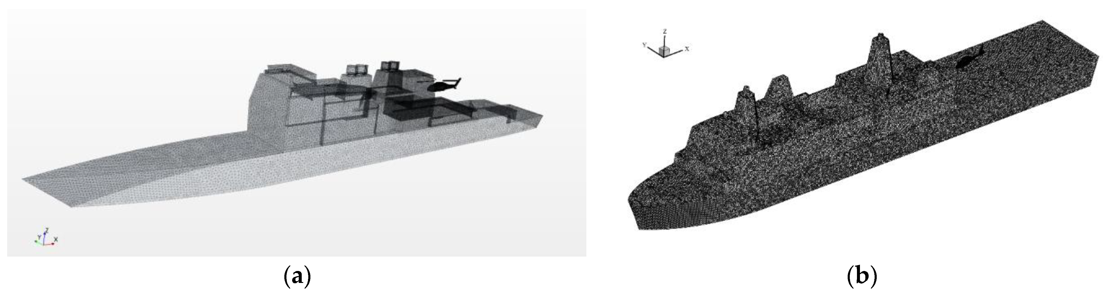
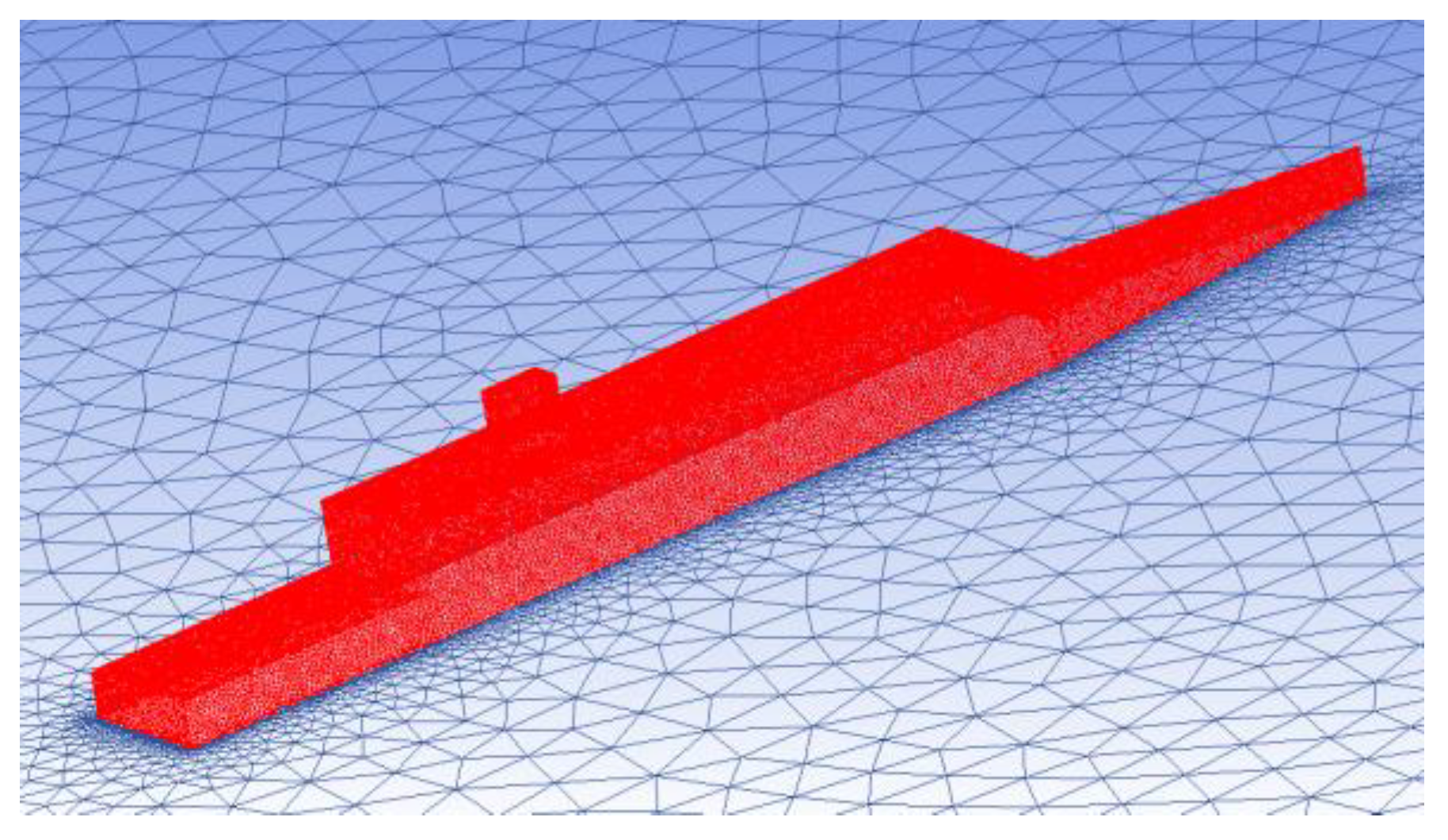
2.6. Numerical Setup

The LPD17 ship equipped with the SA365 Dolphin helicopter and the CG47 ship equipped with the UH60 Black Hawk helicopter is selected as the research sample for calculation and analysis. The established ship models are representative of the actual geometries of the two hulls and most small structures are included. The main geometric and operational parameters of the two sets of ship-helicopter combinations are shown in

Table 1. Main parameters of LPD17 ship and SA365 helicopter.

LPD17 Ship		SA365 Helicopter
Length	208.5 m	Overall Length	13.46 m
Beam	31.9 m	Mass	3850 kg
Speed	22+ knots	Main Rotor (MR) Radius	5.97 m
Maximum Navigational Draft	7 m	MR Rotational Speed	36.55 rad/s
		Number of MR Blades	4
		Tail Rotor (TR) Radius	0.45 m
		Number of TR Blades	13
		TR Rotational Speed	492.80 rad/s

and

Table 2. Main parameters of CG47 ship and UH60 helicopter.

CG47 Ship		UH60 Helicopter
Overall Length	172.82 m	Overall Length	19.76 m
Waterline Beam	16.76 m	Mass	7438.91 kg
Speed	30+ knots	MR Radius	8.18 m
Maximum Navigational Draft	10.2 m	MR Rotational Speed	27 rad/s
		Number of MR Blades	4
		TR Radius	1.68 m
		TR Rotational Speed	124.62 rad/s

.

According to the many studies conducted on simulating ship airwake [4,5,11,16,26], the longitudinal span of the computational domain is between 2.5 and 6 L; the breadth varies between 1–7.5 L; the height range is within 0.63–3.7 L. L is the ship length. In the current study, therefore, the upstream boundary is placed 4 L ahead of the bow and the domain is 10 L long. The width is 20 b (1.94 L) and the height is set as 10 h(1.5 L). b is the ship width and h is the typical ship height. The upstream boundary condition is set as the velocity inlet, and the outlet boundary is defined as the pressure outlet. The lower boundary (sea level) is a no-slip wall. Other boundaries are set as a symmetric plane.

For Combination 1, the grid is generated using the ANSYS ICEM 16.0, a commercial mesh generation software, with tetrahedral elements. The height of the first mesh layer is set to 0.002 m such that the expected non-dimensional wall distance (y+) values are 25 to 65 based on different incoming flow velocities, which satisfies the requirement of the turbulence model. A mesh density box is created to represent the focus region, allowing the flow to be resolved with higher fidelity in the region of interest over the flight deck, as shown in Figure 2 and Figure 3. The total number of mesh cells is 9.2 million. For Combination 2, the automatic meshing facilities of STAR-CCM+ are employed to generate the computational overset mesh. The first grid thickness is also 0.002 m. The tetrahedral unstructured mesh is generated and further mesh refinements are applied to the area surrounding the ship and above the flight deck, as shown in Figure 2 and Figure 3. The overset grid system used for simulations of the Combination 2 is shown in

Table 3. The grid system used for the simulations of Combination 2.

Grid	Cells (Million)
Rotor blade ∗4	1.59 ∗4
Helicopter fuselage	4.01
Background (including ship)	3.80
Total	14.2

. The simulation grid system consists of 6 parts, including four grids for helicopter rotors, one grid for the helicopter fuselage, and one background grid in which the ship is embedded. The total number of mesh cells is 14.2 million.

Each steady simulation for Combination 1 performs at least 20,000 iterations, requiring approximately 50 h of wall-clock time on 24 processors. For the unsteady simulation, the time step should be small enough to capture the dominant vortex frequencies and large enough to prevent the computational time and cost from being too high. For the simulation of isolated ship airwake, 100 time-steps per beam travel time are usually enough to capture the unsteady characteristics of the wake [21]. The frequency of rotor rotation is much larger than that of ship airwake shedding vortex and the rotor simulations are usually conducted with 0.25° to 1° of rotor azimuth per step. Therefore, the determination of time step is based on the rotational speed of the main rotor. In the current study, the time step is set such that the main rotor rotates 2 degrees per time step, equal to 0.001293 s. Although the time-step of 2 degrees per time step is considered to be a large time step for flow-field simulation, it is usually appropriate for obtaining the forces and moments imposed on the helicopter by the airwake. As well, although the time-step is reduced to about 0.5 degrees per time step, the conclusions about the ship’s airwake with the helicopter may not change significantly [22]. The implicit unsteady solver is used and the temporal discretization is second order. Each simulation run calculates a total of 3867 time-steps (about 5 s), equal to about 21 revolutions, requiring approximately 200 h of wall-clock time on 40 processors.

2.7. Rejection Criteria

The first step to be taken to predict the SHOL is to define the so-called rejection criteria for each helicopter type. Rejection criteria are quantitative aircraft parameters and qualitative ratings that, once exceeded, prevent the safe execution of a flight phase [30].

In this study, only objective rejection criteria, including helicopter attitude and control position, are set to predict the SHOL. Note that the steady-state aircraft characteristics are valid for trimmed conditions without any difference between land- or sea-based operations [30]. Therefore, based on the integrated helicopter ground-based operational specifications and previous research experience, the rejection criteria for helicopter landing on the ship flight deck are derived and shown in

Table 4. Rejection criteria for helicopter landing on the ship flight deck.

Variables	Rejection Criteria
Roll angle	>|5°|
Pitch angle	>|8°|
Longitudinal cyclic pitch	>85%
Lateral cyclic pitch	>85%
Collective displacement	>85%
Pedal displacement	>80%

.

2.8. Establishment Method of Candidate SHOL

To ensure safe helicopter shipboard operations in a shipboard environment, the SHOL for a specific ship-helicopter combination is required to determine. The determination of SHOL is generally through at-sea flight tests which are frequently difficult to schedule, time-consuming, expensive, and potentially hazardous [1]. Therefore, developing a simulation method for SHOL predictions to support at-sea flight tests will have clear advantages and attractions. Once the candidate SHOL envelope is established, only the regions with low confidence in the candidate SHOL and/or small safety margins need to be tested, thus significantly reducing the amount of at-sea flight tests.

Based on the proposed rejection criteria previously, the specific process of establishing candidate SHOL is as follows:

• The initial wind direction angle β is 0°;
• Set the initial wind speed V is 0 km/h;
• By using the coupled method, the trimmed control inputs and fuselage attitudes of the shipborne helicopter are calculated;
• Judge whether the rejection criteria are exceeded or not. If they have not been exceeded, the wind speed will increase by 5 km/h, and the iteration is returned to Step 3; if it has been exceeded, the corresponding wind speed is the safety boundary under the current wind direction angle;
• Increase wind direction angle by 30° and return to Step 2 until the wind direction angle covers portside 90° to starboard 90°.

This process is outlined in Figure 4.

3. Results

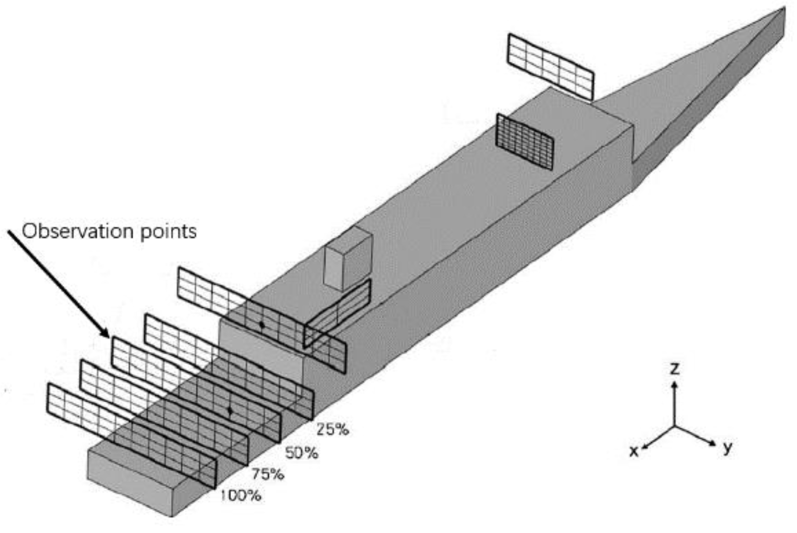
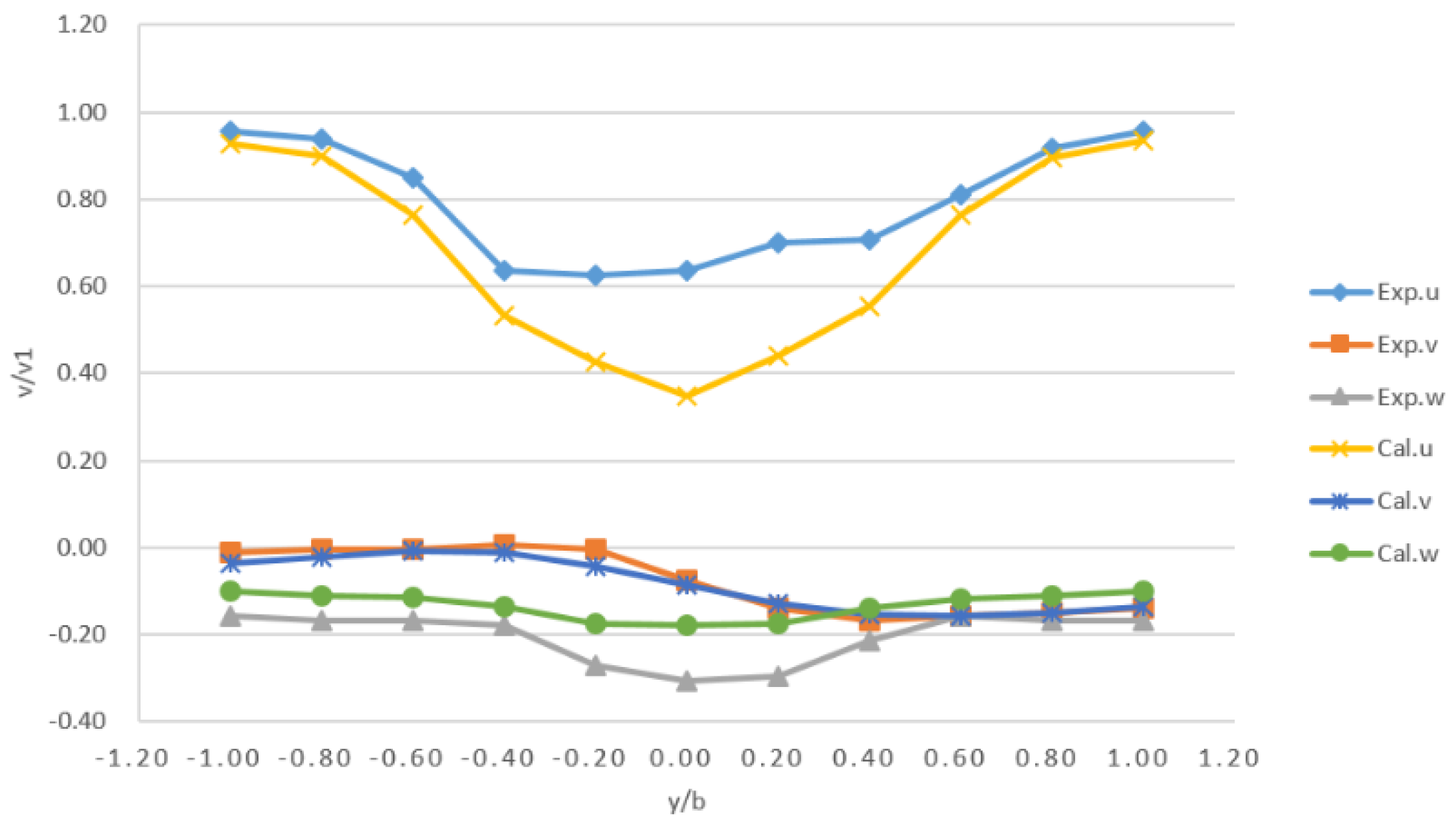
3.1. Validation

Since there is no available experiment data on coupling ship-helicopter flow, the validation of the numerical method is conducted by performing the simulation of the isolated ship. The modification of a simplified frigate model (SFS2) is used for numerical validation. A schematic diagram of SFS2 is shown in Figure 5 (dimensions in feet). The mesh around the SFS2 is shown in Figure 6.

The validation is carried out under the WOD condition of 54 km/h and 0° (headwind). The wind tunnel experiment data are from Ref. [31]. The observation points are located in a horizontal line at the same height as the hangar on the YZ plane at 50% of the flight deck, as shown in Figure 7. The calculated distributions of three velocity components on the observation line are shown in Figure 8, and the corresponding experimental data are also displayed. The horizontal axis is the dimensionless ratio of y-axis coordinates to flight deck width, and the vertical axis is the dimensionless ratio of velocity components to freestream velocity magnitude (V1). From the quantitative comparisons, it can be found that the calculated results show good agreement with the wind tunnel data. The maximum deviation between the two results appears in the velocity in the X direction and is about 0.2. Therefore, the developed method in this paper can be used to explore the ship airwake.

3.2. Mesh Independence Study

A mesh independence study is performed to establish the correct degree of precision. The simulation case is Combination which employs the steady AD model. Three mesh levels are built and denoted: Coarse (5.5 million), Baseline (9.2 million), and Fine (15.6 million). The test WOD condition is set to 0° and 55 km/h. The predicted local speeds along a monitor line over the deck at the height of the fuselage gravity center are compared in Figure 9. It can be observed that the predicted results are similar to these three mesh levels and the results obtained by baseline mesh are closer to those obtained by fine mesh. Therefore, the baseline mesh level (9.2 million) was used in the simulation of Combination 1.

No mesh independence study was performed for the simulation of Combination 2 here. Forrest et al. [32] indicated that five million grids are satisfactory to capture the unsteady flow features for the ship with simple configuration, e.g., SFS2. Considering the higher mesh resolution required by the Detached-Eddy simulation they used, therefore, the mesh number of the background mesh, in which the CG47 is embedded, is set to 3.8 million. In addition, the mesh level of 14.2 million in total can be considered sufficient to capture ship-helicopter aerodynamic interactions, especially considering that many iterations are required for each WOD condition and a large number of WOD conditions need to be simulated.

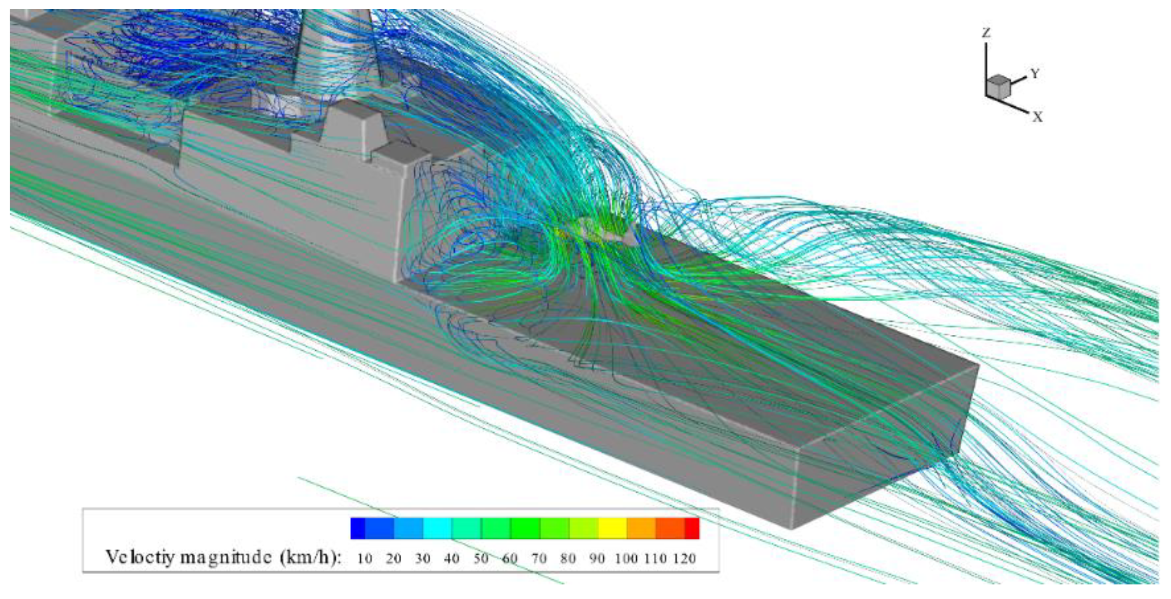
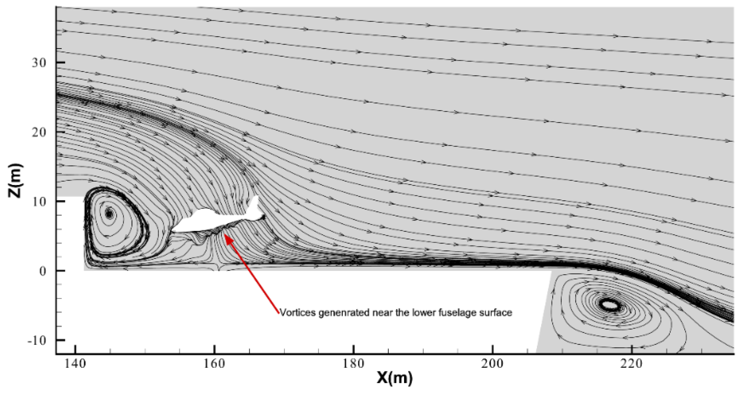
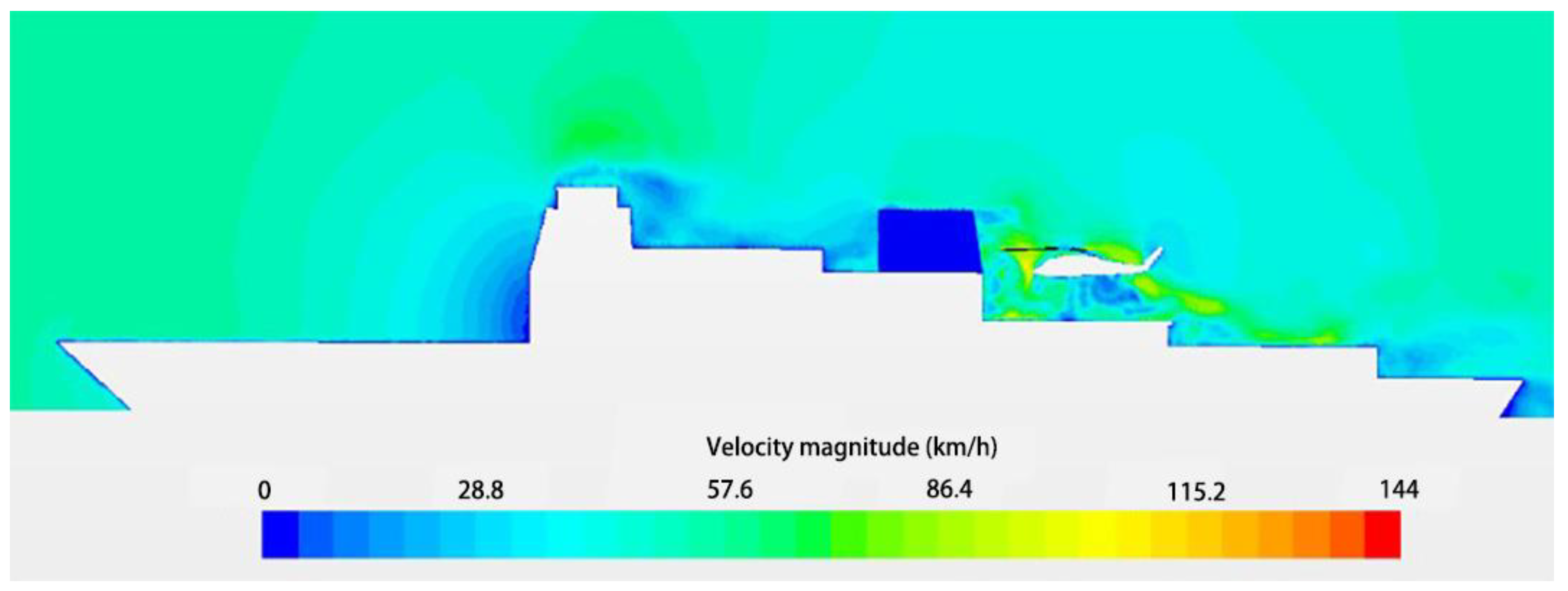
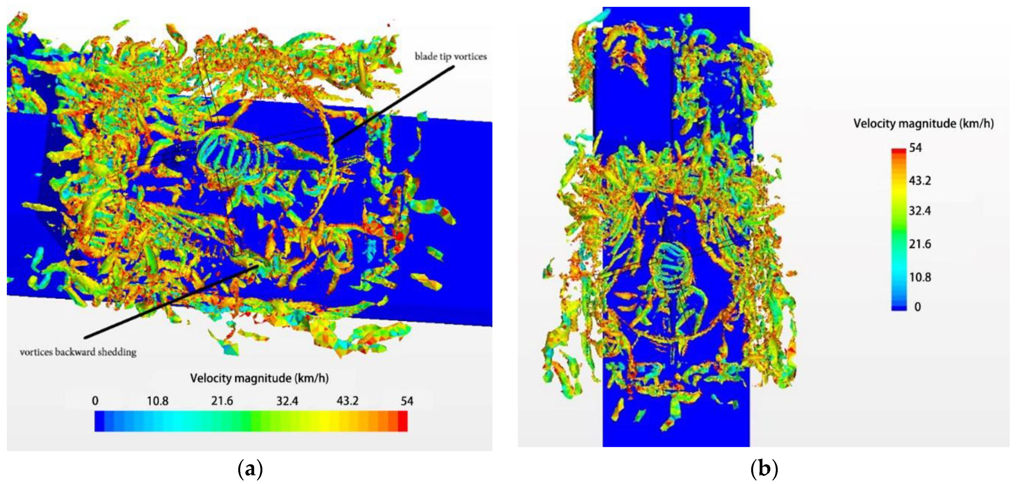
3.3. Fully Coupled Airwake Analysis

In the current study, the fully coupled ship-helicopter airwakes under complete WOD conditions are calculated using two completely different methods for two different ship-helicopter combinations.

3.3.1. Coupled Airwake Topology Analysis for Combination 1

The steady AD model is used in Combination 1 to account for the rotor rotation. It can be seen from Figure 10, Figure 11, Figure 12 and Figure 13 that there are significant interactions between the ship and the helicopter wake.

When the airflow flows through the hangar, a large recirculation zone is generated behind the step and a pair of counterrotating vortices are formed on both sides of this recirculation zone, as shown in Figure 10. Due to the presence of the rotor, the vertical velocity component of the airflow is increased, therefore the reattachment zone points are closer to the hangar, causing a decrease in the size of the recirculation zone. This steep vertical velocity in the airwake over the deck can cause the well-known thrust-deficit phenomenon. The resultant reduction of the available thrust will degrade the pilot’s ability to respond to further fluctuations in lift caused by the unsteady airwake. Moreover, due to the influence of downwash flow on the rotor tip, the boundary layer separation and vortices are generated on the lower surface of the fuselage as seen in Figure 11. These two vortices gradually merge with downwash flow along with the incoming flow. But although the fuselage created a blockage of the rotor-induced downwash, due to its narrow structure, it hardly affects the main flow characteristics of the ship-helicopter coupled flow-field.

As shown in Figure 12 and Figure 13, at portside 30° WOD, the vortex structure of the entire flow-field is no longer symmetrical with respect to the ship’s longitudinal plane. The direction of coupled airwake is inclined towards the ship’s centerline and the dominant vortex rolls over the flight deck. Under the action of the portside wind, the vortex generated at the portside of the hangar falls off from the middle of the deck, forming an area with no large vortex structure on the starboard rear of the entire deck. In such a region, the airflow is gradually unaffected by the superstructure of the ship, which is conducive to the landing of the helicopter. As well, under this condition, the flow field in the portside half of the deck not only has no downwash speed component, but has an upward velocity component. This upwash airflow can increase the rotor thrust. The closer to the rear of the deck, the wider the influence range of upwash airflow. Therefore, under the portside wind conditions, the portside rear of the deck is a reasonable choice of safe landing region. However, it should be noted that when only its portion is exposed to ship airwake, especially to large fluctuations in vertical velocity, the helicopter may experience larger unsteady aerodynamic loads than when the entire helicopter is immersed in ship airwake [1].

As shown in these figures and as predicted based on literature, the results using the steady AD model can correctly capture the main characteristics of the coupled ship-helicopter flow-field and provide a good prediction of the primary steady ship-helicopter interaction. Therefore, the AD model can be used to study the fully coupled ship-helicopter airwake with the consideration of computational efficiency.

3.3.2. Coupled Airwake Topology Analysis of Combination 2

For Combination 2, the resolved blade method based on the overset mesh method is employed to the model rotor. Figure 14 depicts the velocity contour of the longitudinal symmetry plane under 0° and 60 km/h WOD condition. Figure 15 shows the equivalent vorticity map in the vicinity of the flight deck under this WOD condition, colored at local velocity. It can be seen that by using the resolved blade method to simulate the real rotor rotation, the generation of blade tip vortices and the development of vortices backward shedding can be captured more accurately than in the steady AD model.

Due to the complexity of the superstructure of the CG47 ship, when the uniform flow bypasses the superstructure, its speed is reduced and a vortex is generated, causing the uniform flow to become turbulent. As the turbulent airflow continues to flow into the flight deck region, subject to the helicopter rotor, complex vortices are generated with a larger range and greater strength. In such highly turbulent flows, helicopters hovering or landing are much more dangerous and more difficult than on the ground. Therefore, it is necessary to analyze the helicopter flight mechanics characteristics, to understand the changes in the control variables and attitude angles of the helicopter, and to provide effective guidance for a safe landing in the shipboard environment.

3.4. Flight mechanics analysis

Based on the coupling method developed, the flight mechanics analyses of ship-borne helicopters, focusing on helicopter attitude angles and control variables, are carried out under different WOD conditions.

3.4.1. The Influence of Inflow Velocity on Helicopter Landing

Taking Combination 2 as an example, the variations of a helicopter hovering attitude angles and control variables with the inflow speed under a fixed wind direction are analyzed. The variations of roll angle with flow speed under 0° and portside 30° WOD angles are shown in Figure 16, where the horizontal axis represents the inflow speed and the vertical axis represents the trim roll angle under the current WOD condition. It can be derived from Figure 16, that under the same wind direction angle, the helicopter’s trim roll angle has a tendency to increase gradually with inflow speed, which is very unfavorable for helicopters that need to land smoothly. The slope of the curve also increases with inflow speed, indicating that the roll attitude balance of the helicopter will rapidly deteriorate under high wind speed, which may lead to flight accidents. Similarly, the variations of the pitch angle with the inflow speed under 0° and portside 30° WOD angles are given in Figure 17. Under different the wind directions, the trim pitch angle has different trends with the inflow speed, indicating that when landing on the flight deck, the trim attitude of the helicopter does not have a simple linear relationship with the inflow speed but is influenced by many factors, such as the direction and speed of the inflow, as well as the ship superstructure.

Under the same WOD conditions as described above, Figure 18, Figure 19 and Figure 20 show the variations of the helicopter’s main control variables with wind direction, in which the horizontal axis represents the inflow speed and the vertical axis represents the percentage of each control variable to the design maximum. It can be seen that the longitudinal and lateral cyclic pitch control increase with the increase of speed in the same wind direction. This trend is because as the speed increases, the helicopter’s fuselage attitude deviates more from the trimmed position and thus more control forces are required to maintain the attitude. However, when the helicopter is in the vicinity of the flight deck, for safety reasons, the load and vertical landing speed of the helicopter will not change greatly, so the collective pitch control decreases with the increase of the speed.

3.4.2. The Influence of Inflow Angle on Helicopter Landing

In this section, the trim states of the helicopter under different WOD angles are compared while maintaining the same inflow speed. With the increase of the WOD angle, that is, the crosswind speed increases while the forward wind speed decreases, and the helicopter attitude angles change significantly. The pitch angle decreases gradually, while the roll angle increases and deviates to the inflow direction. This trend is also reflected in the cyclic pitch, which decreases in longitudinal and increases in lateral. The collective pitch slightly decreases, mainly because of the wind speed.

Generally speaking, according to the rejection criteria for helicopter landing, each control variable is within the safety margin although it varies considerably. On the contrary, the roll and pitch angles are more likely to exceed the rejection criteria, and become the key indicators affecting the safe landing of shipborne helicopters.

3.5. Candidate SHOL Envelopes

As a critical reference to comprehensively reflect the safety of the ship-helicopter dynamic system, it is necessary to determine the safe operating envelopes for specific ship-helicopter combinations under various WOD conditions, that is, the SHOL envelope [1]. The SHOL predictions derived from the numerical simulations can strongly support at-sea flight tests.

Based on the derived rejection criterion of safe landing and the developed method of establishing a candidate SHOL envelope, the allowable maximum inflow wind speeds under different wind directions are calculated for the two ship-helicopter combinations.

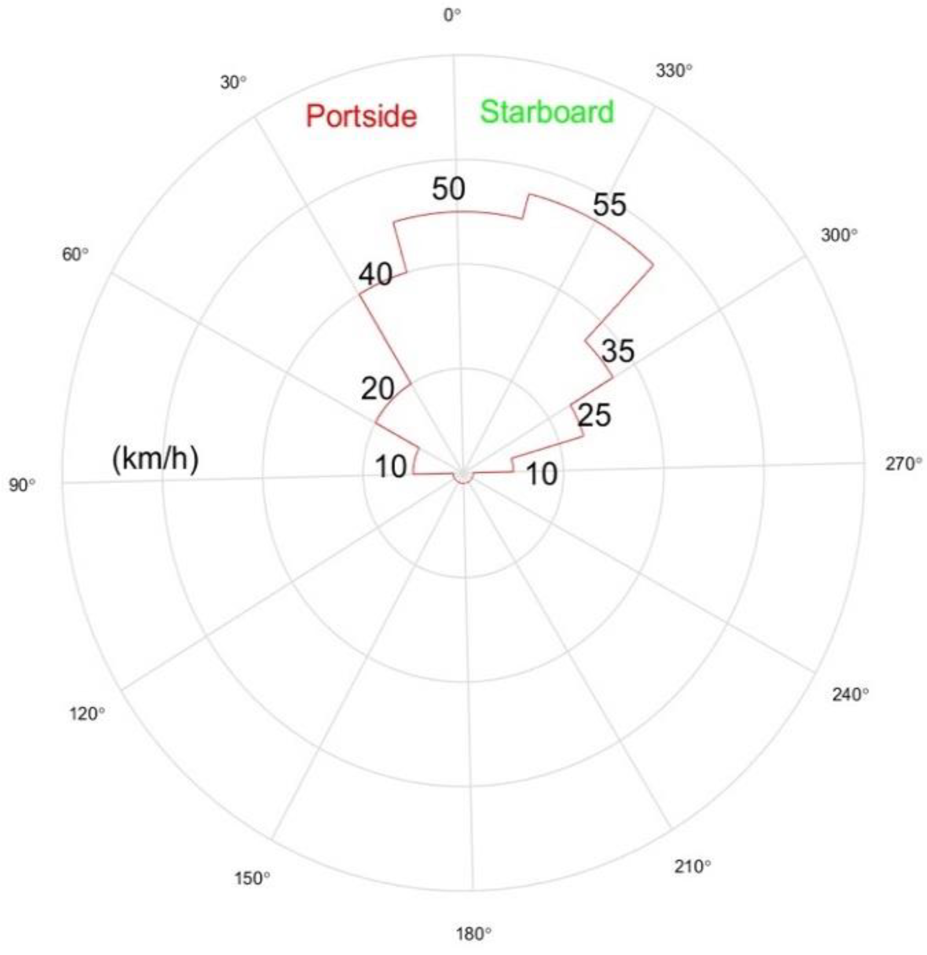
3.5.1. SHOL envelope of Combination 1

The calculated candidate SHOL envelope is shown in Figure 21. It can be seen that small wind direction angles allow larger maximum wind speed and the maximum allowable wind speed occurs at starboard 30°. With the increase of the wind direction angle, the maximum wind speed decreases sharply. This is attributed to the vortex over the whole deck generated by the sharp flight deck edges and the pedal limit caused by greater yawing moment. The lowest tail wind speed is due to the more power required for heading control.

The SHOL envelope exhibits an asymmetrical shape and the maximum wind speed under the starboard wind angle is greater than that under the corresponding portside wind angle. The main rotor of the SA365 helicopter has counterclockwise rotation, so the pull direction of the tail rotor is left to overcome the counter-torque of the main rotor. The starboard wind is equivalent to increasing the collective pitch of the tail rotor, increasing the available control margin. Therefore, the SA365 helicopter itself has a stronger ability to resist the starboard wind, which determines that it should choose to enter from the starboard when landing. When the wind is coming from the portside, the helicopter is in the recirculation zone formed by the hangar, which is extremely harmful for safe take-off and landing. As well, the relative movement between the helicopter and the ship leads to the increase in relative wind speed. The existence of these factors will inevitably lead to the helicopter’s ability to resist the portside wind being weaker than the ability to resist the starboard wind. With the increase of the wind direction angle, the recirculation zone decreases as its location changes, reducing the difference between the starboard and portside.

Although there is no SHOL envelope of such a ship-helicopter combination as a reference, the analysis of the flow-field characteristics under different WOD conditions obtained by CFD simulation implies that the calculated SHOL envelope is reasonable. Therefore, the steady AD model can be used in the study of helicopter operations in a shipboard environment, especially considering the computational efficiency.

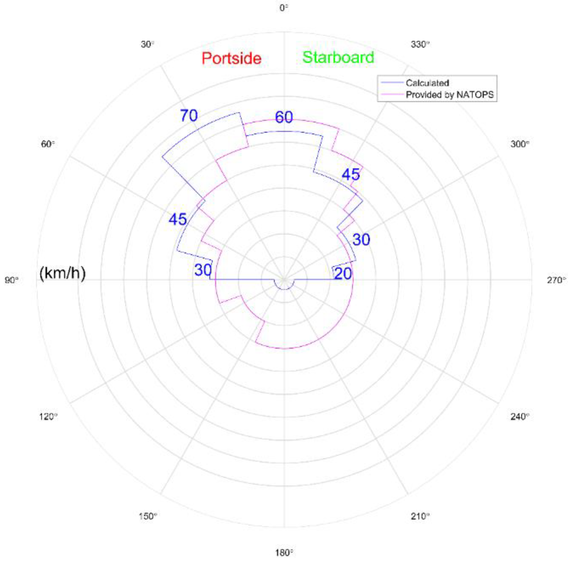
3.5.2. SHOL Envelope of Combination 2

The calculated SHOL envelope of Combination 2 is shown in Figure 22. The launch and recovery envelope of this combination provided by the NATOPS manual are also shown in this figure. The calculated SHOL envelope shows reasonable agreement with the envelope provided by the NATOPS for the same helicopter-ship combination without recovery assistance. The differences may be due to the fact that the established numerical method does not consider the helicopter landing procedure, the ship motion, and the pilot workload. Therefore, the established simulation method could be employed as a tool to obtain a preliminary candidate SHOL envelope to support an at-sea flight test.

The maximum allowable wind speed varies greatly under different wind directions. In general, the closer the inflow wind direction is to the ship head, the larger the maximum allowable wind speed is. The crosswind causes a rapid decrease in the maximum allowable wind speed. The SHOL envelope of Combination 2 shows similar characteristics to that of Combination 1. The SHOL envelope of Combination 2 is also asymmetrical. But contrary to the SHOL envelope of Combination 1, the maximum allowable wind speed under the portside wind condition for Combination 2 is generally larger than that under the starboard condition. This is because the UH60 helicopter has a clockwise rotor and the tail rotor pulls to the right, making it more capable of dealing with the portside wind. As well, the maximum allowable wind speed for Combination 2 is significantly larger than that for Combination 1, which is attributed to the helicopter flight speed and the ship geometry characteristics.

4. Conclusions

Employing a steady AD model and resolved blade method, the fully coupled ship-helicopter flow-field simulations are conducted over two ship-helicopter combinations (LPD17-SA365 and CG47-UH60) under various WOD conditions. Based on the established HFM model, flight mechanics characteristics of the two combinations are studied and analyzed. As well, according to the proposed rejection criteria and developed numerical method, the candidate SHOL envelopes of the two combinations are derived. The results indicate that:

• It is indicated that the developed coupling method and establishment method of candidate SHOL is a promise simulation tool for the analysis of the mutual ship-helicopter interactions and SHOL predictions to support at-sea flight tests;
• The results confirm that numerical simulation of shipborne helicopters using both steady AD model and resolved blade method can accurately capture the main characteristics of the fully coupled ship-helicopter flow-field;
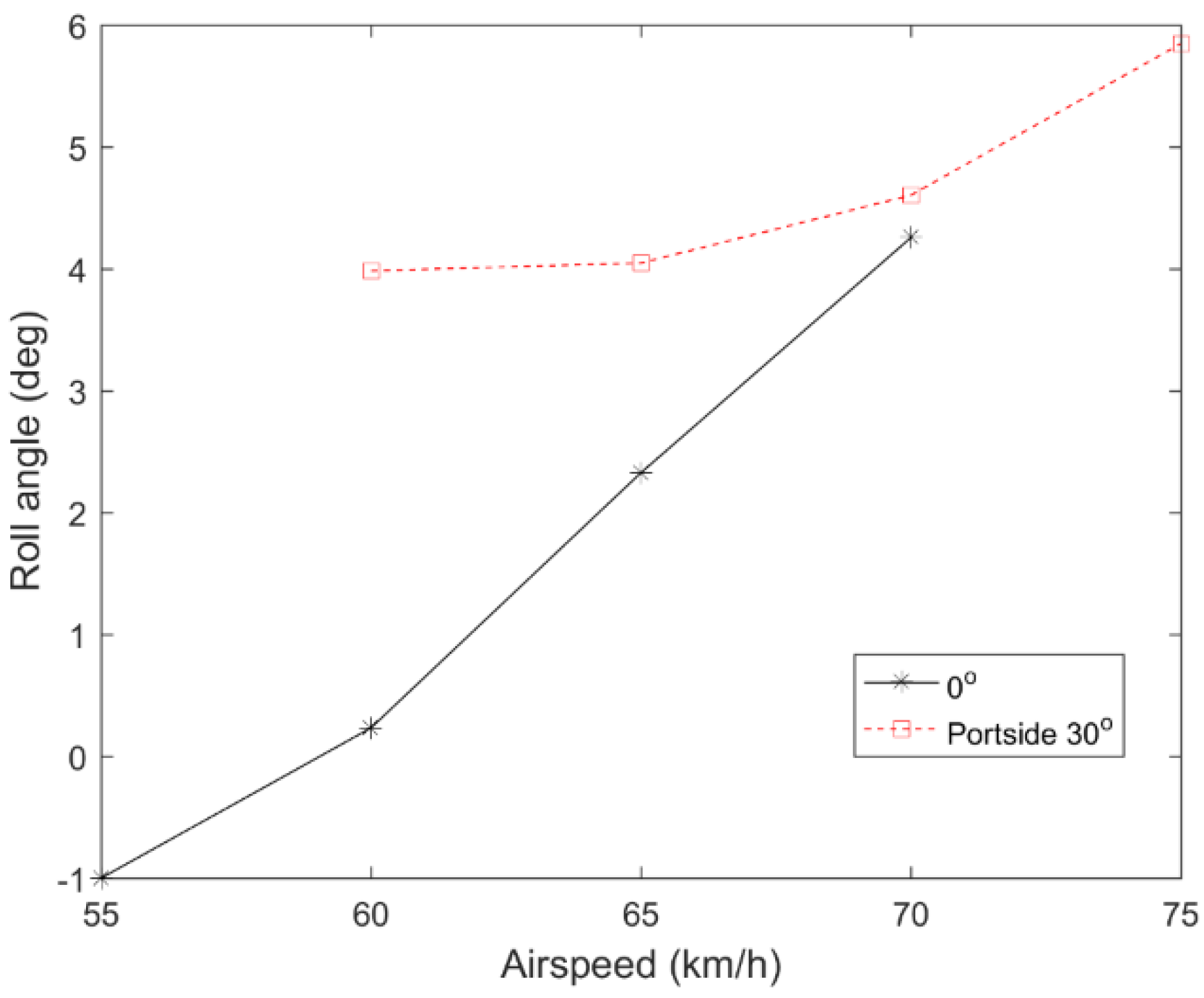
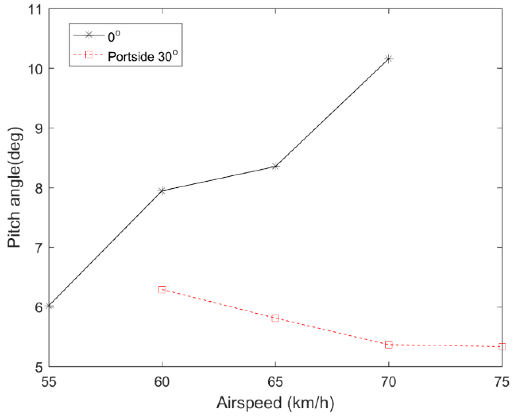
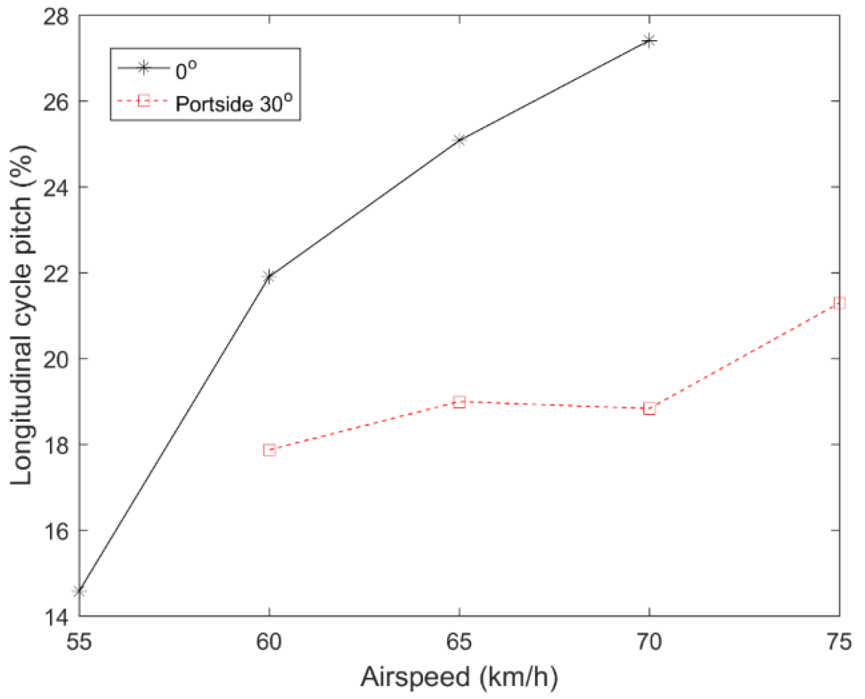
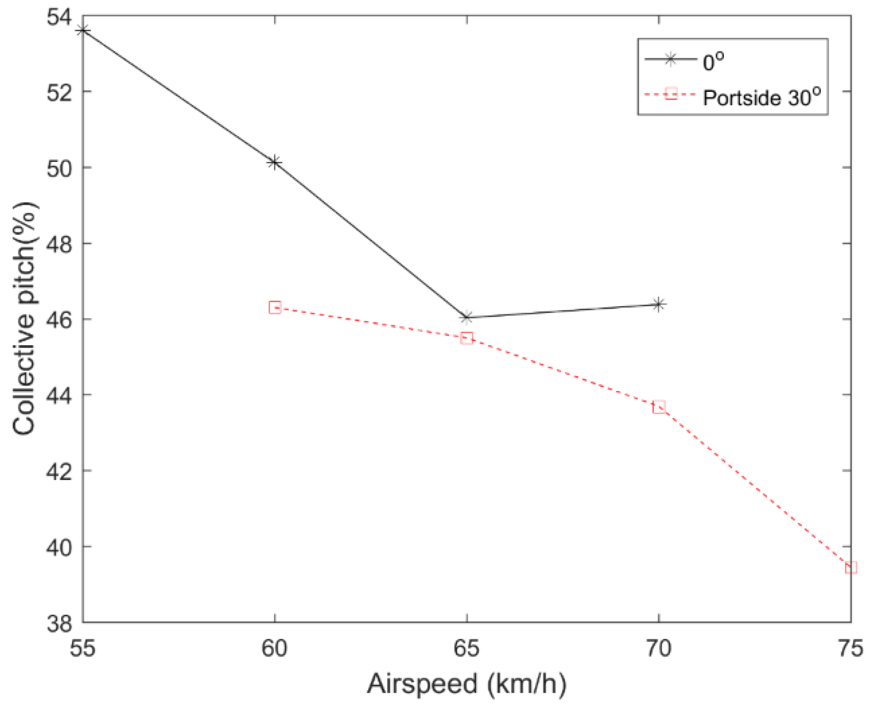
• The flight mechanics analysis of Combination 2 shows that under the same wind angle condition, the helicopter’s trim roll angle tends to increase with the inflow wind speed. The pitch angle does not have a simple linear relationship with the inflow speed but is subject to inflow direction and ship superstructure. The longitudinal and lateral cyclic control displacements increase with the wind speed;
• The analysis of Combination 2 indicates that under the same inflow wind speed, with the increase of wind direction angle, the pitch angle decreases while the roll angle increases and deviates to the inflow wind direction. This trend is also reflected in the cyclic pitch, which decreases in longitudinal and increases in lateral;
• The roll and pitch angles are more likely to exceed the rejection criteria, and become the key indicators affecting the safe landing of shipborne helicopters;
• From the derived candidate SHOL envelopes of the two combinations, it can be found that the maximum allowable inflow wind speed varies greatly under different wind directions. The allowable wind speed is larger in the case of a small wind direction angle and the maximum wind speed occurs at 30 degrees for both ship-helicopter combinations;
• The SHOL envelopes are both asymmetrical. For Combination 1, the SHOL on the portside is generally larger than that on the starboard; while the SHOL envelope of Combination 2 shows the opposite characteristic. These differences are mainly due to the rotation direction of the main rotors.

References

- Cao, Y.; Qin, Y. Insight into the factors affecting the safety of take-off and landing of the ship-borne helicopter. Proc. Inst. Mech. Eng. Part G J. Aerosp. Eng. 2022, 236, 1925–1946. [Google Scholar] [CrossRef]
- Cao, Y.; Qin, Y. Modeling and Simulation of Ship–Helicopter Dynamic Interface: Method and Application. Arch. Comput. Methods Eng. 2022, 1–41. [Google Scholar] [CrossRef]
- Forrest, J.S.; Hodge, S.J.; Owen, I.; Padfield, G.D. An investigation of ship airwake phenomena using time-accurate CFD and piloted helicopter flight simulation. In Proceedings of the 34th European rotorcraft forum, Liverpool, UK, 16–19 September 2008. [Google Scholar]
- Lee, D.; Sezer-Uzol, N.; Horn, J.F.; Long, L.N. Simulation of Helicopter Shipboard Launch and Recovery with Time-Accurate Airwakes. J. Aircr. 2005, 42, 448–461. [Google Scholar] [CrossRef]
- Oruc, I.; Horn, J.F.; Polsky, S.; Shipman, J.; Erwin, J. Coupled flight dynamics and CFD simulations of the helicopter/ship dynamic interface. In Proceedings of the 71st American Helicopter Society annual forum, Virginia, VA, USA, 5–7 May 2015. [Google Scholar]
- Kääriä, C.H.; Forrest, J.S.; Owen, I. The virtual AirDyn: A simulation technique for evaluating the aerodynamic impact of ship superstructures on helicopter operations. Aeronaut. J. 2013, 117, 1233–1248. [Google Scholar] [CrossRef]
- Forrest, J.; Kaaria, C.; Owen, I. Evaluating ship superstructure aerodynamics for maritime helicopter operations through CFD and flight simulation. Aeronaut. J. 2016, 120, 1578–1603. [Google Scholar] [CrossRef]
- Memon, W.A.; Owen, I.; White, M.D. SIMSHOL: A Predictive Simulation Approach to Inform Helicopter–Ship Clearance Trials. J. Aircr. 2020, 57, 854–875. [Google Scholar] [CrossRef]
- Zan, S.J. On Aerodynamic Modelling and Simulation of the Dynamic Interface. Proc. Inst. Mech. Eng. Part G J. Aerosp. Eng. 2005, 219, 393–410. [Google Scholar] [CrossRef]
- Bridges, D.; Horn, J.; Alpman, E.; Long, L. Coupled Flight Dynamics and CFD Analysis of Pilot Workload in Ship Airwakes. In Proceedings of the AIAA Atmospheric Flight Mechanics Conference and Exhibit, Hilton Head, SC, USA, 20–23 August 2007. [Google Scholar] [CrossRef] [Green Version]
- Wakefield, N.H.; Newman, S.J.; Wilson, P. Helicopter flight around a ship‘s’ superstructure. Proc. Inst. Mech. Eng. Part G J. Aerosp. Eng. 2002, 216, 13–28. [Google Scholar] [CrossRef]
- Alpman, E.; Long, L.N.; Bridges, D.O.; Horn, J.F. Fully-Coupled Simulations of the Rotorcraft/Ship Dynamic Interface. In Proceedings of the American Helicopter Society 63rd Annual Forum, Virginia Beach, VA, USA, 1–3 May 2007. [Google Scholar]
- Le Chuiton, F. Actuator disc modelling for helicopter rotors. Aerosp. Sci. Technol. 2004, 8, 285–297. [Google Scholar] [CrossRef]
- Tang, L.; Dinu, A.; Polsky, S. Reduced-Order Modeling of Rotor-Ship Interaction. In Proceedings of the 50th AIAA Aerospace Sciences Meeting, Nashville, TN, USA, 9–12 January 2012. [Google Scholar] [CrossRef]
- Rajmohan, N.; Zhao, J.; He, C.; Polsky, S. Development of a Reduced Order Model to Study Rotor/Ship Aerodynamic Interaction. In Proceedings of the AIAA SciTech Forum, Kissimmee, FL, USA, 5–9 January 2015. [Google Scholar] [CrossRef]
- Lu, Y.; Chang, X.; Chuang, Z.; Xing, J.; Zhou, Z.; Zhang, X. Numerical investigation of the unsteady coupling airflow impact of a full-scale warship with a helicopter during shipboard landing. Eng. Appl. Comput. Fluid Mech. 2020, 14, 954–979. [Google Scholar] [CrossRef]
- Crozon, C.; Steijl, R.; Barakos, G. Numerical Study of Helicopter Rotors in a Ship Airwake. J. Aircr. 2014, 51, 1813–1832. [Google Scholar] [CrossRef]
- Oruc, I.; Horn, J.F.; Shipman, J. Coupled Flight Dynamics and Computational Fluid Dynamics Simulations of Rotorcraft/Terrain Interactions. J. Aircr. 2017, 54, 2228–2241. [Google Scholar] [CrossRef]
- Lee, Y.; Silva, M. CFD-Modeling of Rotor Flowfield Aboard Ship. In Proceedings of the 48th AIAA Aerospace Sciences Meeting, Orlando, FL, USA, 4–7 January 2010. [Google Scholar] [CrossRef]
- Lawson, S.; Woodgate, M.; Steijl, R.; Barakos, G. High performance computing for challenging problems in computational fluid dynamics. Prog. Aerosp. Sci. 2012, 52, 19–29. [Google Scholar] [CrossRef]
- Crozon, C.; Steijl, R.; Barakos, G. Coupled flight dynamics and CFD—demonstration for helicopters in shipborne environment. Aeronaut. J. 2018, 122, 42–82. [Google Scholar] [CrossRef] [Green Version]
- Dooley, G.; Martin, J.E.; Buchholz, J.H.; Carrica, P.M. Ship Airwakes in Waves and Motions and Effects on Helicopter Operation. Comput. Fluids 2020, 208, 104627. [Google Scholar] [CrossRef]
- Yakhot, V.; Orszag, S.A.; Thangam, S.; Gatski, T.B.; Speziale, C.G. Development of turbulence models for shear flows by a double expansion technique. Phys. Fluids 1992, 4, 1510–1520. [Google Scholar] [CrossRef]
- Syms, G. Numerical Simulation of Frigate Airwakes. Int. J. Comput. Fluid Dyn. 2004, 18, 199–207. [Google Scholar] [CrossRef]
- Kulkarni, P.; Singh, S.; Seshadri, V. Parametric studies of exhaust smoke–superstructure interaction on a naval ship using CFD. Comput. Fluids 2007, 36, 794–816. [Google Scholar] [CrossRef]
- Reddy, K.; Toffoletto, R.; Jones, K. Numerical simulation of ship airwake. Comput. Fluids 2000, 29, 451–465. [Google Scholar] [CrossRef]
- Roper, D.M.; Owen, I.; Padfield, G.D.; Hodge, S.J. Integrating CFD and piloted simulation to quantify ship-helicopter operating limits. Aeronaut. J. 2006, 110, 419–428. [Google Scholar] [CrossRef]
- Talbot, P.D.; Tinling, B.E.; Decker, W.A.; Chen, R.T. A Mathematical Model of a Single Main Rotor Helicopter for Piloted Simulation; NASA-TM-84281; National Aeronautics and Space Administration: Washington, DC, USA, 1 September 1982.
- Cao, Y.; Cao, L.; Wan, S. Trim Calculation of the CH-53 Helicopter Using Numerical Continuation Method. J. Guid. Control Dyn. 2014, 37, 1343–1349. [Google Scholar] [CrossRef]
- Hoencamp, A.; Pavel, M.D. Concept of a Predictive Tool for Ship–Helicopter Operational Limitations of Various In-Service Conditions. J. Am. Helicopter Soc. 2012, 57, 032008. [Google Scholar] [CrossRef]
- Roper, D.M.; Owen, I.; Padfield, G.D. CFD investigation of the helicopter-ship dynamic interface. In Proceedings of the 61st American Helicopter Society International Annual Forum, Grapevine, TX, USA, 1–3 June 2005. [Google Scholar]
- Forrest, J.S.; Owen, I. An investigation of ship airwakes using Detached-Eddy Simulation. Comput. Fluids 2010, 39, 656–673. [Google Scholar] [CrossRef]