Development of Recovery System for Underwater Glider

Abstract

This study proposes a novel autonomous system that is able to retrieve an underwater glider safely and quickly. After a long-period mission, the glider is out of its energy, floats up in the middle of the sea, and needs retrieval. However, most of the recovery processes are conducted manually, which is not effective and even damages the glider or injures the worker. In this study, we propose the use of a remotely operated vehicle (ROV) in a recovery process that consists of three stages: (i) driving the ROV into the near area of the glider, (ii) automatically catching the glider using the ROV’s onboard sensors and capturing mechanisms, and (iii) retrieving the glider to the mother ship or station. Mathematical models were formulated to realize the feasibility of the system. A cascade adaptive sliding mode control-proportional integral controller is designed to cope with the thruster’s characteristics, the dynamics of the ROV and the glider, and oceanic disturbances. Finally, simulation studies were conducted in the system operation scenarios and their results validate the efficiency of the proposed process.

1. Introduction

Nowadays, the use of ocean data is becoming popular in marine engineering and ecosystem management. Thanks to this information, complex tasks such as typhoon prediction, whale ecological monitoring, and red tide monitoring can be conducted reliably. In order to collect the necessary oceanographic data, underwater gliders carrying multiple instruments and communication systems have been developed and deployed. The gliders are a type of non-holonomic autonomous underwater vehicle (AUV) that employs buoyancy propulsions instead of propellers or thrusters. By switching between negative and positive buoyancies, the gliders follow an up-and-down sawtooth-like trajectory very slowly but consume very little energy. Therefore, they offer a significantly greater range and endurance. Hence, they are able to perform ocean sampling missions from hours to weeks or months, and to thousands of kilometers of range [1,2,3]. After these long-period missions, the gliders float up in the middle of the sea, are unable to return by themselves, and required retrieving. In other cases, such as a glider being damaged or drifting out of its planned trajectory, rescue missions are also required. Unfortunately, recovering a glider is always a challenging task.

The conventional approach is to use human skills and rudimentary equipment, such as nets, cranes, belts, and hooks, to bring back a glider, as depicted in Figure 1. For example, the Argo project [4,5] comprises 3000 underwater gliders scattered throughout the world’s oceans. To recover a glider to check and calibrate it before the next mission, a mother ship approached the location the glider had sent. The worker dropped the net below and then pulled it towards the glider so that the glider fits in the net. The two were then lifted by a crane, and workers used their strength to pull them back to the mother ship. The succession of the work relies on the experience and skills of the operators. Moreover, the glider may collide with the ship and recovery equipment such that its body and instruments take damage. In bad weather conditions, not only does the retrieving task become more difficult, but the risk of accidents to people also increases. Therefore, a safe and automatic glider recovery method is necessary.

On the other hand, numerous projects have been conducted on recovery AUVs, which have a similar structure and dynamical characteristics to the glider. A favorite recovery method is to control the AUV to dock into a capture mechanism such as a funnel, net, and pole [6,7,8,9]. The docking procedure is generally as follows: the AUV follows a global path to approach the station; determines the location and posture of the dock station; generates the docking path; and finally, follows the guidance and enters the docking cabin. The docking process is possible thanks to the maneuverability of a traditional AUV. Unfortunately, for the non-holonomic AUVs, the docking maneuver is more challenging. The complexity of the maneuver and the influence of the turbulence environment cause the docking process to fail easily and damage the AUV. Especially for an uncontrollable glider after its mission, the process is not possible. Several studies designed a docking cabin that is movable by being carried by a submarine [10] or surface vehicle [11]. However, the succession of docking still relies on the AUV’s motion performance.

Then comes the use of other types of vehicles to retrieve an AUV; some still require a certain level of operation of the AUV, while others just control the retrieving vehicle without controlling the AUV. Multi-propeller aerial vehicles have been deployed in [12] for not only recovery but also deployment of the AUVs. The recovery mechanism first uses a line and hook and then evolves by utilizing an electro-permanent magnet to capture and release the AUV. The line and hook put risk on both vehicles, but the other mechanism shows its capability. However, the airflow generated by the propellers creates large turbulence over the water and disturbs the position of the vehicle to be recovered. Remotely operated vehicles (ROVs) were used to recover submerged vehicles in [13,14]. The ROVs were equipped with a camera and a gripper so that their operator can search and capture the submerged assets remotely. Unfortunately, it was difficult for the operator to estimate the position and the distance between the two vehicles from the camera’s perspective. Sarda et al. [15,16] designed an AUV recovery system based on unmanned surface vehicles. The recovery involves lowering a thin line with an outrigger-type depressor wing from the winch on the surface vehicle, latching the line with the AUV using a pincer-type onboard mechanism, and finally, reeling the line for vehicle retrieval. For the process, the AUV has to be submerged underwater. Moreover, lining up the recovery mechanism is not easily done with only the controlled motion of the surface vehicles. Thus, different mechanisms are designed and examined, such as funnel recovery [17], and wing and rope capturing [18] devices.

Due to its great potential, surface vehicle-based systems have been considered for glider recovery; for example, in the study of Howse et al. [9]. Since the glider floats on the surface of the ocean, which is different from the AUV, the surface vehicle is designed with the Small Waterplane Area Twin Hull (SWATH) form. The recovery mechanism uses a net with linkages helping it catch and lift the glider in a similar way to the manual operation. Hence, disadvantages of manual operation remain, such as the risk of damaging the glider and the difficulty of controlling the recovery system. Other approaches require modifying significantly the glider [19,20,21] such that it has autonomous recovery capability. Apparently, it cannot recover itself when running out of energy. Nevertheless, very few studies have considered the problem of automatic glider recovery in our knowledge. The process still heavily relies on manual operation, which is full of risks and drawbacks.

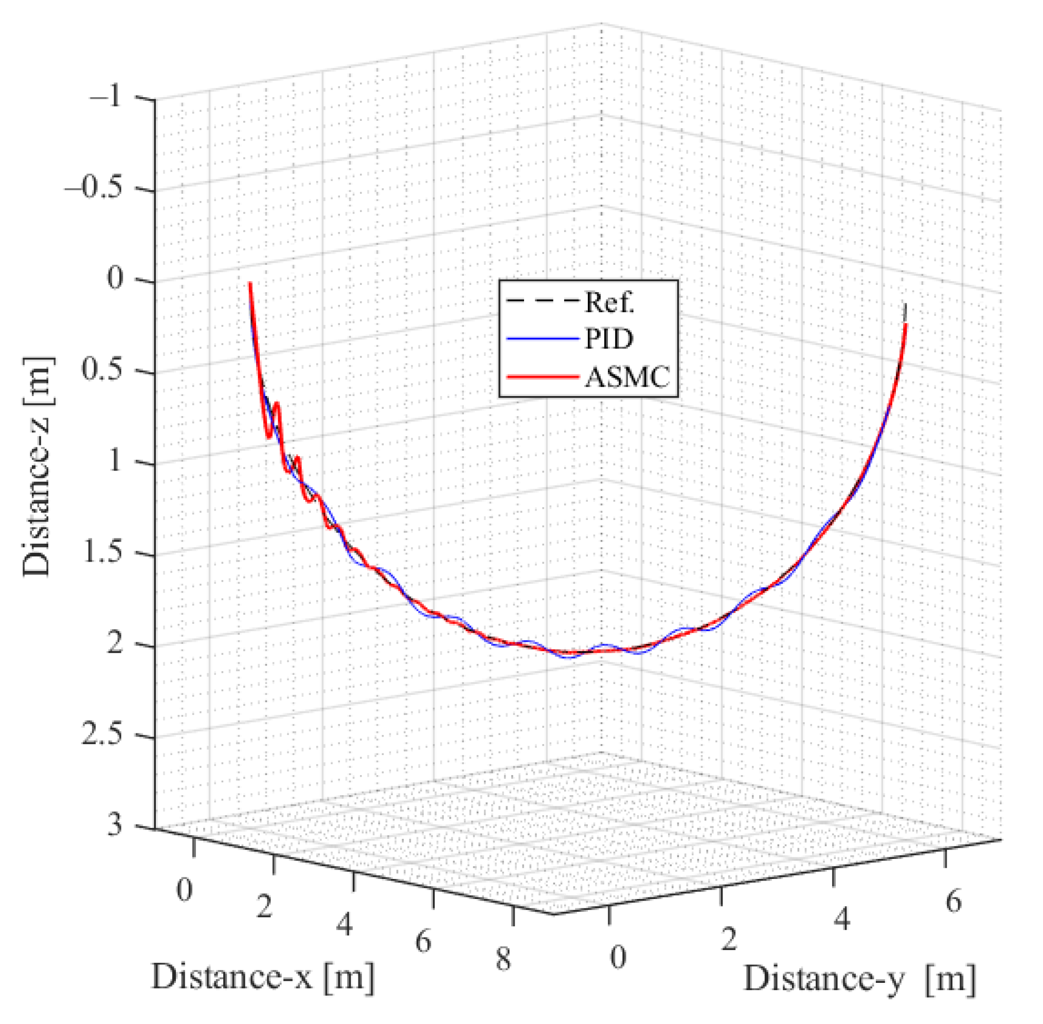
Therefore, in this study, we propose a novel glider recovery method using a ROV. The vehicle is renovated with additional instruments and mechanisms for the objective of capturing and retrieving the glider. The recovery process consists of three stages: (i) driving the ROV to the neighborhood area below the glider, (ii) determining the position and orientation of the glider and catching it, and (iii) retrieving the glider to the mother ship or station. In order to analyze the maneuverability of the recovery system, the mathematical model is firstly derived, and a cascade adaptive sliding mode control (ASMC)-proportional integral (PI) control system is then designed. Simulation studies in the operation scenario of the system show its feasibility. Comparison results with a cascade proportional integral derivative (PID)-PI also validate the effectiveness of the proposed system. Then, the contributions of this paper can be summarized as follows:

-

A novel recovery method for the underwater glider using the ROV is proposed.

-

The mathematical model of the ROV is derived while taking the process (dynamics of the recovered glider, hydrodynamics, buoyancy effects, etc.) into the formulation

-

The cascade ASMC-PI control system is designed. The system stability is proved by the Lyapunov-like lemma. The system’s effectiveness and robustness are validated through comparative simulations.

The remainder of the paper is organized into 5 sections. Section 2 introduces the proposed glider recovery process. The mathematical model of the system is derived in Section 3. The design of the cascade ASMC-PI control system is presented in detail in Section 4, whereas its control performance is discussed in Section 5. Finally, conclusions are drawn in Section 6.

2. Proposed Glider Recovery Process

In this study, the propeller-type ROV is used to recover the target underwater glider. For this objective, the ROV first needs to determine the position and posture of the glider. We place a stereo camera in the front of the ROV, and the lighting system ensures we can obtain good vision even when submerging. Numerous studies proposed reliable methods to detect and estimate the posture of an object with this visual data, for example in [22,23,24,25]. The ROV also uses the sensors such as an inertial measurement unit (IMU) and global positioning system (GPS) to measure its own position and rotation. The ROV is equipped with a gripper and a clamp for capturing and carrying the glider. The gripper picks up the hook underneath the glider, which is a minor accessory added to the glider. The clamp is kept fully opening while the ROV is deployed from the mother ship or operating station. After picking up, the ROV adjusts its posture so that the clamp holds tightly the upper body of the glider when closing up. Then, the glider moves together with the ROV and is retrieved. The structure of the renovated ROV is depicted in Figure 2.

With this ROV, the proposed glider recovery process involves three stages:

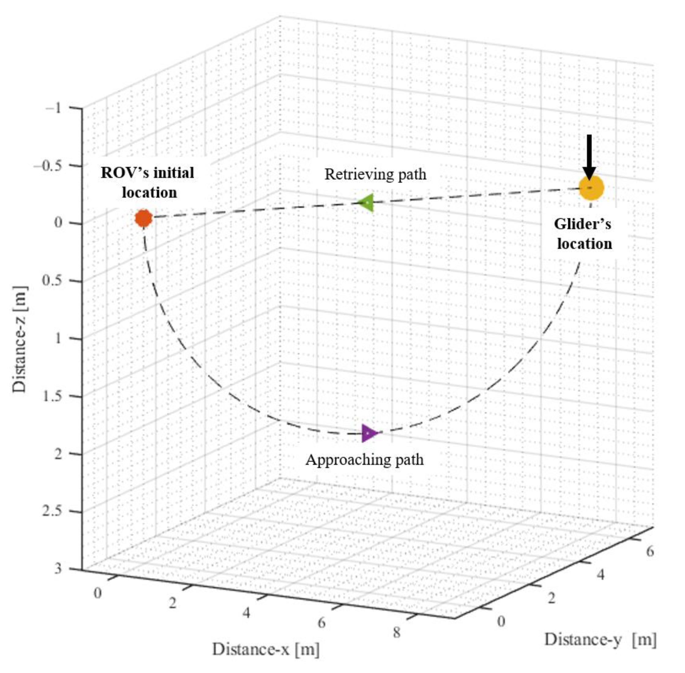
Approaching stage: After localizing the glider to be recovered, the ROV is deployed from the mother ship or operating station. It follows a global trajectory, avoids obstacles, and avoids colliding with the glider’s body. The ROV reaches a destination point below the glider, points toward it, and then switches to the next stage.

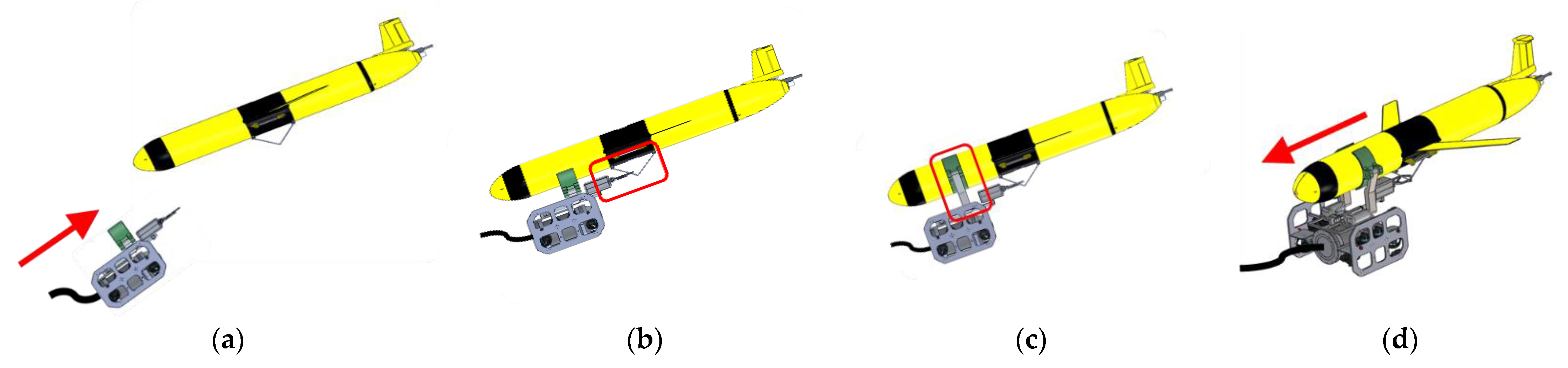
Capturing stage: Through the visual data obtained from the stereo camera, the position and orientation of the glider in the ROV-fixed coordinates are determined. A path planning algorithm, for example [26], generates the required movements for the ROV, including the movement to the pick-up point for the gripper and the subsequent rotation to a position parallel to the glider. The posture estimation and path planning tasks are conducted similarly to those in the docking operations mentioned in the literature review. The difference is that those tasks are conducted by the ROV instead of the vehicle to be recovered. The ROV performs the motion as follows: (i) It follows the guidance to the pick-up point for the gripper; (ii) the gripper catches the hook beneath the glider; (iii) the ROV rotates following the given guidance; and (iv) the clamp holds the upper body of the glider. These motions are illustrated in Figure 3.

Retrieving stage: The ROV carries the glider back to the mother ship or station.

It is worth noting the second stage requires completely autonomous operation. This is due to the close distance between two vehicles, thus resulting in a high precision requirement. Besides, an operator has the difficulty in estimating the absolute position and the depth from the camera perspective. The motion path in other stages can be either remotely given by the operator or automatically generated by the path planning algorithm. The control system has to give an effective and robust performance in the whole process.

3. System Modeling

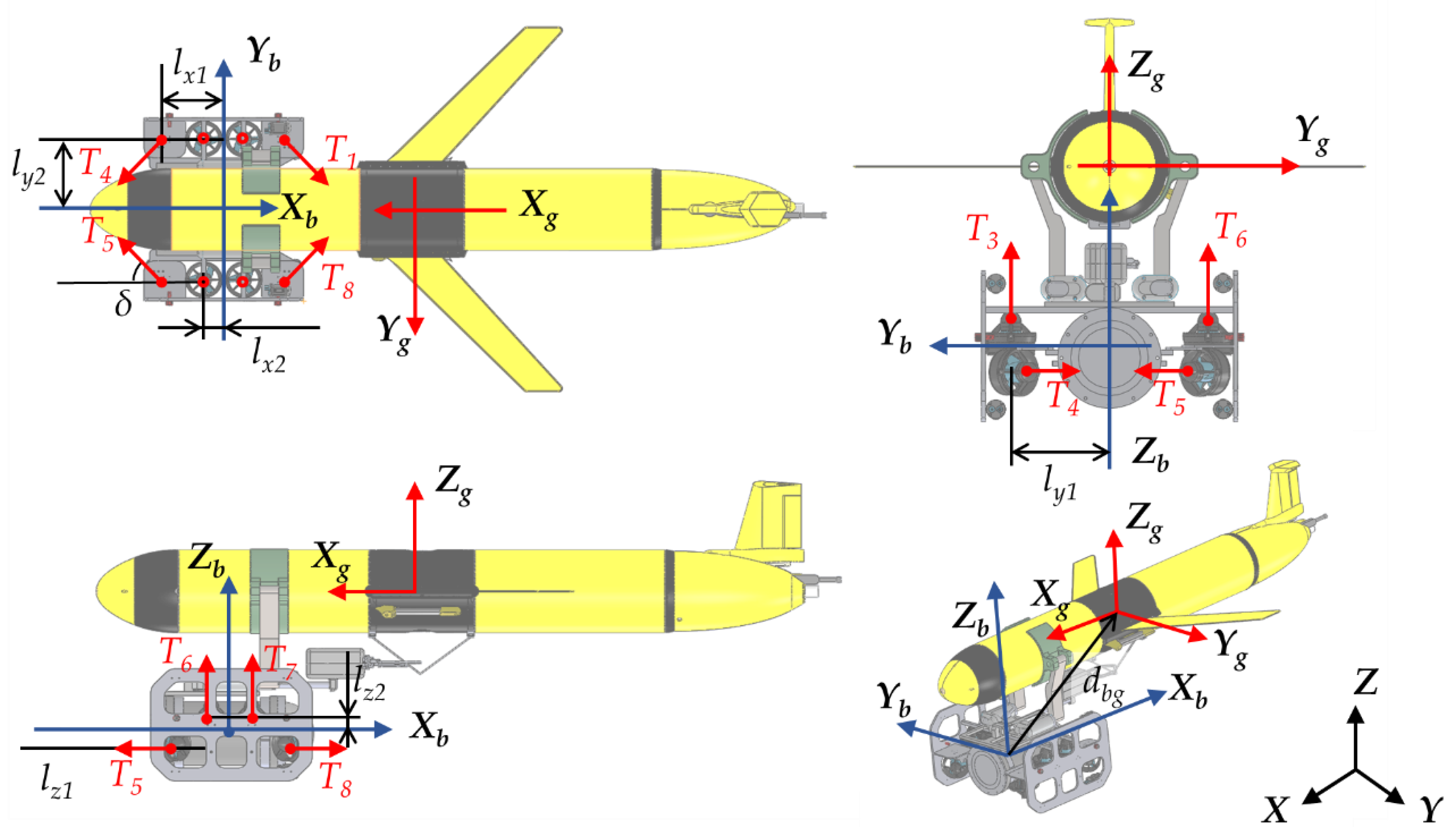
In order to analyze the maneuverability of the recovery system, the system dynamics are formulated. We consider the motions in three coordinates: the Earth-fixed frame (or inertial frame) XYZ, the ROV’s body-fixed frame X_bY_bZ_b and the glider-fixed frame X_gY_gZ_g. They are depicted in Figure 4. Key dimensions of the ROV, as well as the actuating thrust forces, are also shown in the figure.

The rigid-body dynamics of the ROV submerged in water, including hydrodynamic drag and added mass parameters, are as follows [27,28]:

$$\begin{array}{c}\dot{\eta }=J(\eta )\nu ,\\ M\dot{\nu }=-C(\nu )\nu -D(\nu )\nu -g(\eta )+\tau +{\tau }_C+{\tau }_G\end{array}$$

(1)

where:

$\eta ={\left[\begin{array}{cccccc}x& y& z& \varphi & \theta & \psi \end{array}\right]}^T$ is the vector containing the position and the orientation of the body frame with respect to the Earth-fixed frame. The orientation is represented by three Euler angles of roll, pitch, and yaw in XYZ order.

$\nu ={\left[\begin{array}{cccccc}u& v& w& p& q& r\end{array}\right]}^T$ is the state vector of body-frame linear and angular velocities.

$J(\eta )$ is the transformation matrix from the body frame to the inertial frame. It is given by:

$$\begin{array}{c}J(\eta )=\left[\begin{array}{cc}{R}_B^I& O_3\\ O_3& J_{k,o}^{-1}\end{array}\right],\\ R_B^I={\left[\begin{array}{ccc}{c}_{\psi }{c}_{\theta }& s_{\psi }{c}_{\theta }& -s_{\theta }\\ -s_{\psi }{c}_{\varphi }+c_{\psi }{s}_{\theta }{s}_{\varphi }& c_{\psi }{c}_{\theta }+s_{\psi }{s}_{\theta }{s}_{\varphi }& s_{\varphi }{c}_{\theta }\\ s_{\psi }{s}_{\varphi }+c_{\psi }{s}_{\theta }{c}_{\varphi }& -c_{\psi }{s}_{\varphi }+s_{\psi }{s}_{\theta }{c}_{\varphi }& c_{\varphi }{c}_{\theta }\end{array}\right]}^{-1},\hspace{0.17em}\hspace{0.17em}\hspace{0.17em}\hspace{0.17em}{J}_{k,o}^{-1}=\frac{1}{c_{\theta }}\left[\begin{array}{ccc}{c}_{\theta }& s_{\varphi }{s}_{\theta }& c_{\varphi }{s}_{\theta }\\ 0& c_{\varphi }{c}_{\theta }& -s_{\varphi }{c}_{\theta }\\ 0& s_{\varphi }& c_{\varphi }\end{array}\right]\end{array}$$

(2)

with $c_{(\hspace{0.17em}\cdot \hspace{0.17em})}=\cos (\hspace{0.17em}\cdot \hspace{0.17em})$ and $s_{(\hspace{0.17em}\cdot \hspace{0.17em})}=\sin (\hspace{0.17em}\cdot \hspace{0.17em})$.

M denotes the matrix of the ROV’s mass and inertia including added mass and inertia parameters due to hydrodynamic effects. The matrix is diagonal if the origin of the body-fixed frame is chosen coincident with the central frame and the body is completely submerged in the water, the velocity is low, and it has three planes of symmetry.

$$\begin{array}{c}M=M_{AUV}+M_A,\\ M_{AUV}=\left[\begin{array}{cc}m{I}_3& O_3\\ O_3& J\end{array}\right],\\ M_A=-diag\left(X_{\dot{u}},Y_{\dot{v}},Z_{\dot{w}},K_{\dot{p}},M_{\dot{q}},N_{\dot{r}}\right)\end{array}$$

(3)

where m and J are the ROV’s own mass and inertia tensor. $diag\left(X_{\dot{u}},Y_{\dot{v}},Z_{\dot{w}}\right)$ contains the added mass and $diag\left(K_{\dot{p}},M_{\dot{q}},N_{\dot{r}}\right)$ is the added inertial. $O_3$ and $I_3$ are the 3-by-3 zeros and identity matrices, respectively.

$C(\nu )$ is the nonlinear Coriolis and centripetal matrix. As in [27,28], $C(\nu )$ is introduced as follows:

$$\begin{array}{c}C(\nu )=C_{AUV}(\nu )+C_A(\nu ),\\ C_{AUV}(\nu )=\left[\begin{array}{cccccc}0& 0& 0& 0& mw& -mv\\ 0& 0& 0& -mw& 0& mu\\ 0& 0& 0& mv& -mu& 0\\ 0& mw& -mv& 0& J_{z}r& -J_{y}q\\ -mw& 0& mu& -J_{z}r& 0& J_{x}p\\ mv& -mu& 0& J_{y}q& -J_{x}p& 0\end{array}\right],\hspace{0.17em}\hspace{0.17em}\hspace{0.17em}\hspace{0.17em}\hspace{0.17em}{C}_A(\nu )=\left[\begin{array}{cccccc}0& 0& 0& 0& -Z_{\dot{w}}w& Y_{\dot{v}}v\\ 0& 0& 0& Z_{\dot{w}}w& 0& -X_{\dot{u}}u\\ 0& 0& 0& -Y_{\dot{v}}v& X_{\dot{u}}u& 0\\ 0& -Z_{\dot{w}}w& Y_{\dot{v}}v& 0& -N_{\dot{r}}r& M_{\dot{q}}q\\ Z_{\dot{w}}w& 0& -X_{\dot{u}}u& Y_{\dot{v}}v& 0& -K_{\dot{p}}p\\ -Y_{\dot{v}}v& X_{\dot{u}}u& 0& -M_{\dot{q}}q& K_{\dot{p}}p& 0\end{array}\right]\end{array}$$

(4)

The diagonal, linear, and quadratic hydrodynamic drag matrix is denoted by $D(\nu )$ and they are given by:

$$D(\nu )=-diag\left(X_u,Y_v,Z_w,K_p,M_q,N_r\right)\hspace{0.17em}-diag\left(X_{u\left|u\right|}\left|u\right|,Y_{v\left|v\right|}\left|v\right|,Z_{w\left|w\right|}\left|w\right|,K_{p\left|p\right|}\left|p\right|,M_{q\left|q\right|}\left|q\right|,N_{r\left|r\right|}\left|r\right|\right)$$

(5)

with the coefficients of $D(\nu )$ being considered to be constant.

$g(\eta )$ is the restoring force and moment vector that combines gravitational and buoyancy effects. In the ROV’s body-fixed frame, the ROV’s center of gravity is at $r_G^B={\left[\begin{array}{ccc}0& 0& 0\end{array}\right]}^T$ and its center of buoyancy is at $r_B^B={\left[\begin{array}{ccc}{x}_B& y_B& z_B\end{array}\right]}^T$. Then, the restoring force and moment vector is obtained by:

$$g(\eta )=\left[\begin{array}{c}\left(m-\rho \nabla \right)g{s}_{\theta }\\ -\left(m-\rho \nabla \right)g{c}_{\theta }{s}_{\varphi }\\ -\left(m-\rho \nabla \right)g{c}_{\theta }{c}_{\varphi }\\ \rho \nabla g\left(y_B{c}_{\theta }{c}_{\varphi }-z_B{c}_{\theta }{s}_{\varphi }\right)\\ \rho \nabla g\left(-z_B{s}_{\theta }-x_B{c}_{\theta }{c}_{\varphi }\right)\\ \rho \nabla g\left(x_B{c}_{\theta }{s}_{\varphi }+y_B{s}_{\theta }\right)\end{array}\right]$$

(6)

In which, g is the gravitational acceleration, ρ is the water density, and $\nabla$ the volume of the body underwater.

The vector of control force and moment is denoted by $\tau$ and resulted from the thrust vector T generated by the thruster assembly. From the configuration of the thrusters shown in Figure 4, $\tau$ relates to the thrusts via the thruster configuration matrix as follows:

$$\begin{array}{c}\tau =K_{T}T,\\ T={\left[\begin{array}{cccccccc}{T}_1& T_2& T_3& T_4& T_5& T_6& T_7& T_8\end{array}\right]}^T,\\ K_T=\left[\begin{array}{cccccccc}{c}_{\delta }& 0& 0& -c_{\delta }& -c_{\delta }& 0& 0& c_{\delta }\\ -s_{\delta }& 0& 0& -s_{\delta }& s_{\delta }& 0& 0& s_{\delta }\\ 0& 1& 1& 0& 0& 1& 1& 0\\ -l_{z1}{s}_{\delta }& l_{y2}& l_{y2}& -l_{z1}{s}_{\delta }& l_{z1}{s}_{\delta }& -l_{y2}& -l_{y2}& l_{z1}{s}_{\delta }\\ -l_{z1}{c}_{\delta }& -l_{x2}& l_{x2}& l_{z1}{c}_{\delta }& l_{z1}{c}_{\delta }& l_{x2}& -l_{x2}& -l_{z1}{c}_{\delta }\\ -l_{x1}{s}_{\delta }-l_{y1}{c}_{\delta }& 0& 0& l_{x1}{s}_{\delta }+l_{y1}{c}_{\delta }& -l_{x1}{s}_{\delta }-l_{y1}{c}_{\delta }& 0& 0& l_{x1}{s}_{\delta }+l_{y1}{c}_{\delta }\end{array}\right]\end{array}$$

(7)

In addition, the dynamics of the thrusters generate thrust is assumed to follow the hydrodynamic linear model [29]. For the ith thruster, the model is presented by:

$$\begin{array}{c}{\dot{n}}_i=-k_{1i}{n}_i-k_{2i}{Q}_i(n_i,{\upsilon }_i)+k_{3i}{u}_i,\\ {\dot{\upsilon }}_i=-k_{4i}\left({\upsilon }_i-U\right)\left|{\upsilon }_i-U\right|+k_{5i}{T}_i(n_i,{\upsilon }_i),\\ T_i(n_i,{\upsilon }_i)=c_{n_i}^T{n}_i\left|n_i\right|-c_{n_i{\upsilon }_i}^T\left|n_i\right|{\upsilon }_i,\\ Q_i(n_i,{\upsilon }_i)=c_{n_i}^Q{n}_i\left|n_i\right|-c_{n_i{\upsilon }_i}^Q\left|n_i\right|{\upsilon }_i\end{array}$$

(8)

where n_i and ${\upsilon }_i$ are the ith propeller angular velocity and the axial fluid velocity, respectively. $T_i(n_i,{\upsilon }_i)$ and $Q_i(n_i,{\upsilon }_i)$ represent its thrust output and reaction torque. U is the ambient velocity. k_ji (j = 1,2,3,4) are positive definite, so are the parameters $c_{n_i}^T$, $c_{n_i{\upsilon }_i}^T$, $c_{n_i}^Q$ and $c_{n_i{\upsilon }_i}^Q$. Additionally, $u_i$ is the actuator’s voltage to be controlled.

Moreover, the effects of waves, wind, and, especially, ocean currents are denoted by ${\tau }_C$. By assuming the current irrotational and constant in the earth-fixed frame, its effects can be modeled as follows:

$${\tau }_C=-\left[\begin{array}{cc}{R}_I^B& O_3\\ O_3& R_I^B\end{array}\right]{\theta }_{\upsilon C}$$

(9)

with ${\theta }_{\upsilon C}$ the vector of constant parameters contributing to the earth-fixed generalized forces and moments due to the current.

Finally, ${\tau }_G$ is the vector of resistance force and moment from the glider acting on the ROV. That means before retrieving the glider, ${\tau }_G=0$, and after the ROV catches the glider, ${\tau }_G$ is resultant from the glider motion. The latter case is formulated by:

$$\begin{array}{c}{\tau }_G=-K_G\left(M_G\dot{\nu }+C_G(\nu )\nu +D_G(\nu )\nu +g_G(\eta )-{\tau }_{GC}\right),\\ K_G=\left[\begin{array}{cc}{I}_3& O_3\\ S(d_{bg})& I_3\end{array}\right]\end{array}$$

(10)

where $d_{bg}={\left[\begin{array}{ccc}{d}_x& d_y& d_z\end{array}\right]}^T$ is the vector of translation from the origin of the ROV’s body-fixed frame to the mass center of the glider. $S(d_{bg})$ denotes the skew-symmetrical matrix of $d_{bg}$. $M_G$, $C_G(\nu )$, and $D_G(\nu )$ are, respectively, the mass and inertia matrix, the Coriolis and centripetal matrix, and the drag matrix of the glider. Finally, $g_G(\eta )$ and ${\tau }_{GC}$ are the forces and moments acting on the glider and are modeled in a similar manner to those of the ROV. It is noted that since the glider is tightly held by the ROV, its translational and rotational velocities in the ROV’s body-fixed frame is the same as those of the ROV.

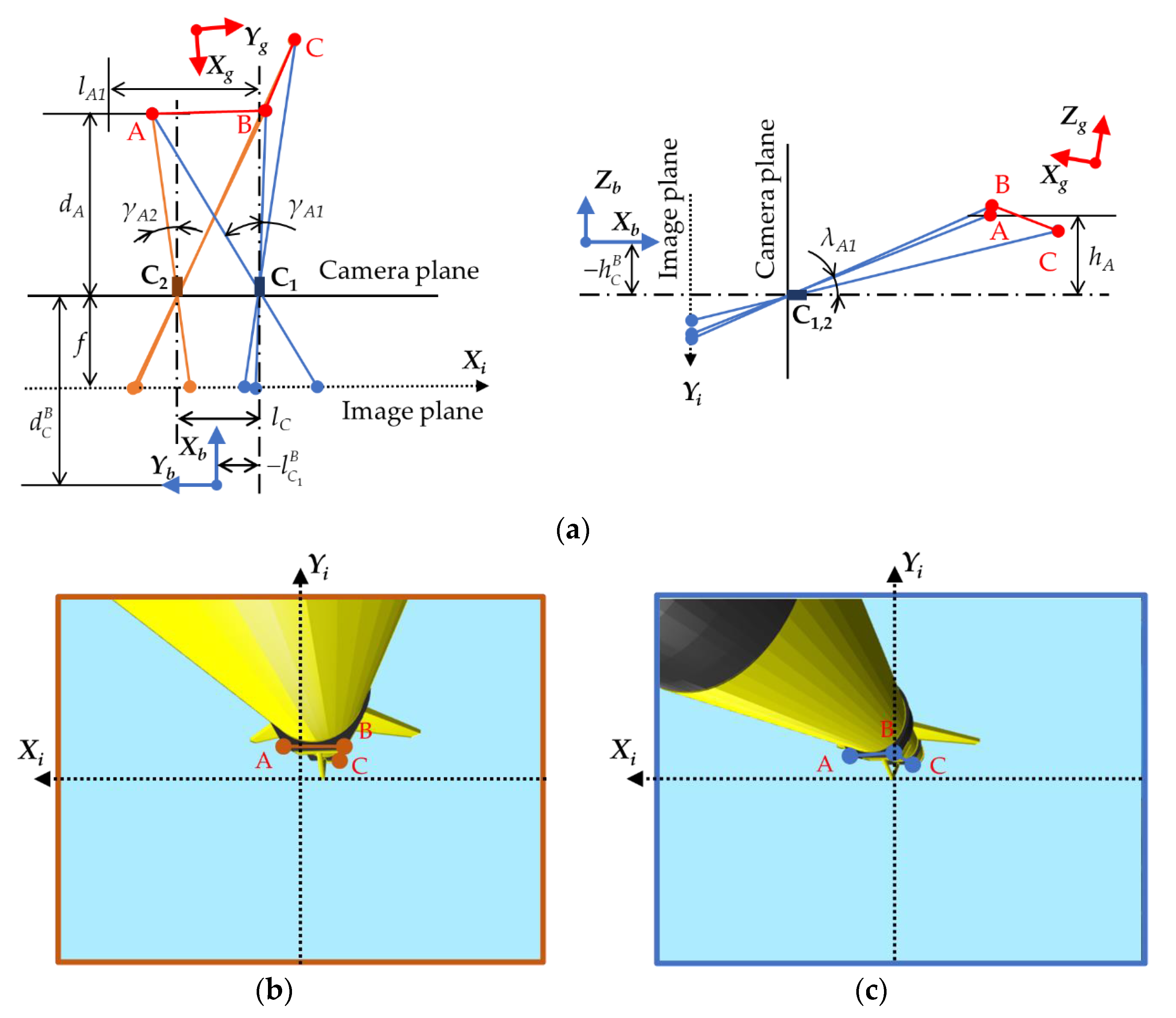
On the other hand, it is worth noting that in the second stage of the glider recovery process, both the position and orientation of the glider are required to be measured so that the glider can be captured successfully. In other words, the representation of the glider-fixed frame relative to the ROV’s body-fixed frame must be obtained. Moreover, if one can derive the position in this frame of at least three certain points of the glider, the relative position and orientation of the glider are completely defined. This is done using the stereo camera system in this study. Figure 5 illustrates the 6-dimensional pose estimation of the glider in this stage using the stereo camera system on the ROV, in which the position of a point A on the glider’s body expressed in the ROV’s body-fixed frame is computed by:

$$\begin{array}{c}{\left[\begin{array}{ccc}{x}_A^B& y_A^B& z_A^B\end{array}\right]}^T={\left[\begin{array}{ccc}{d}_C^B+d_A& l_{C_1}^B+l_{A1}& h_C^B+h_A\end{array}\right]}^T,\\ d_A=\frac{l_{C}f}{-x_A^{C_1}{S}_x^{C_1}+x_A^{C_2}{S}_x^{C_2}},\hspace{0.17em}\hspace{0.17em}\hspace{0.17em}\hspace{0.17em}{l}_{A1}=-d_A\frac{x_A^{C_1}{S}_x^{C_1}}{f},\hspace{0.17em}\hspace{0.17em}\hspace{0.17em}\hspace{0.17em}{h}_A=-\frac{y_A^{C_1}{S}_y^{C_1}}{f{d}_A}\end{array}$$

(11)

where $x_A^{C_1}$ and $y_A^{C_1}$ represent the projection of A on the horizontal and vertical coordinates, respectively, of the image plane of the right camera (camera C₁). $S_x^{C_1}$ and $S_y^{C_1}$ are the horizontal and vertical size of a pixel. f denotes the focal length and ${\left[\begin{array}{ccc}{d}_C^B& l_{C_1}^B& h_C^B\end{array}\right]}^T$ is the location of camera C₁ in the ROV’s body-fixed frame. Finally, $l_C$ is the distance between the two cameras in the stereo camera system.

4. Motion Control System Design

The objective of the motion control system is to operate the ROV’s thrusters such that the ROV follow the desired paths of motion, both before and after retrieving the glider. In practical operations, the desired paths are given by an operator, in the case of remote control of the ROV, or from a motion planning algorithm based on the position of the glider and the measurement system equipped in the ROV. To fulfill the control objective, a cascade control structure is proposed. In the outer control loop, the sliding mode control law computes the force and moment for the ROV to reach its desired motion. In the inner loop, each thruster is controlled by the PI controller such that it generates thrust as required. In order to effectively cope with disturbances and uncertainties, an adaptive law is added to the control system.

Assume that the voltage input of each thruster can be mapped to its generated thrust such that $T_i=K_{ui}{u}_i$. Then to the total force and moment acting on the ROV. This can be done by either a variety of models, such as linear gains or nonlinear dead-zone functions [30,31], or experimental tests. Then, the dynamics model of AUV in Equation (1) can be rearranged as follows:

$$\begin{array}{c}\dot{\eta }=J_B^I(\eta )\nu ,\\ M\dot{\nu }=-C(\nu )\nu -D(\nu )\nu -g(\eta )+{\tau }_u+{\tau }_{u,d}+{\tau }_C+{\tau }_G\end{array}$$

(12)

where ${\tau }_u$ is the vector of force and moment mapped from the thrusters’ voltage input $u$. ${\tau }_{u,d}$ is the remaining dynamical terms between $\tau$ and $u$. Let us assume that these dynamics can be approximated by first-order models. Moreover, Equation (12) can be rewritten entirely in the Earth-fixed frame, to eliminate the terms expressed in the body-fixed frame, as follows [27,28,32,33]:

$$M_{\eta }\ddot{\eta }+\left({\Lambda }_{\eta }+\mathsf{\Delta }{\Lambda }_{\eta }\right)\dot{\eta }+g_{\eta }(\eta )+d_{\tau }={\tau }_{u,\eta }$$

(13)

In which:

$$\begin{array}{c}{M}_{\eta }={\left(J_B^I(\eta )\right)}^{-T}M{\left(J_B^I(\eta )\right)}^{-1},\\ {\Lambda }_{\eta }+\mathsf{\Delta }{\Lambda }_{\eta }=C_{\eta }(\nu ,\eta )+D_{\eta }(\nu ,\eta ),\hspace{0.17em}\\ d_{\tau }=-{\tau }_C{}_{,\eta }-{\tau }_G{}_{,\eta }-{\tau }_{u,d}{}_{,\eta }\end{array}$$

(14)

and

$$\begin{array}{c}{C}_{\eta }(\nu ,\eta )={\left(J_B^I(\eta )\right)}^{-T}\left(C\left(\nu \right)-M{\left(J_B^I(\eta )\right)}^{-1}{\dot{J}}_B^I(\eta )\right){\left(J_B^I(\eta )\right)}^{-1},\\ D_{\eta }(\nu ,\eta )={\left(J_B^I(\eta )\right)}^{-T}D\left(\nu \right){\left(J_B^I(\eta )\right)}^{-1},\hspace{1em}{g}_{\eta }(\eta )={\left(J_B^I(\eta )\right)}^{-T}g(\eta ),\\ {\tau }_{u,d}{}_{,\eta }={\left(J_B^I(\eta )\right)}^{-T}{\tau }_{u,d},\hspace{1em}{\tau }_C{}_{\eta }={\left(J_B^I(\eta )\right)}^{-T}{\tau }_C,\hspace{1em}{\tau }_G{}_{\eta }={\left(J_B^I(\eta )\right)}^{-T}{\tau }_G,\hspace{0.17em}\hspace{0.17em}\hspace{0.17em}{\tau }_{u,\eta }={\left(J_B^I(\eta )\right)}^{-T}{\tau }_u\end{array}$$

(15)

The term ${\Lambda }_{\eta }$ represents the nominal value of $C_{\eta }(\nu ,\eta )+D_{\eta }(\nu ,\eta )$, and $\mathsf{\Delta }{\Lambda }_{\eta }$ denotes the remaining uncertainty. The uncertainty $\mathsf{\Delta }{\Lambda }_{\eta }$ and the disturbance $d_{\tau }$ are assumed to be bounded and satisfy the matching condition.

For a given vector ${\eta }_d$ of the desired position and orientation of the ROV in the Earth-fixed frame, let the tracking error be defined as $e=\eta -{\eta }_d$. A vector of sliding surfaces is considered as follows:

$$s=\dot{e}+K_{s}e$$

(16)

With $K_s$ a positive diagonal matrix. $s$ converges to zero equivalent to the asymptotic stability of the ROV.

From Equations (13)–(16), the following dynamics of the sliding surfaces is obtained:

$$\begin{array}{c}\dot{s}=M_{\eta }^{-1}\left({\tau }_{u,\eta }-{\Lambda }_{\eta }\dot{\eta }-g_{\eta }(\eta )\right)-{\ddot{\eta }}_d+K_s\dot{e}+D_e\left(\dot{\eta },\tau \right),\\ D_e\left(\dot{\eta },\tau \right)=M_{\eta }^{-1}\left[-\mathsf{\Delta }{\Lambda }_{\eta }\dot{\eta }-d_{\tau }\right]\end{array}$$

(17)

$D_e\left(\dot{\eta },\tau \right)$ denotes the total effect of the uncertainties and disturbances on the sliding surface. In order to guarantee that the sliding variable converges to zero, even with the presence of uncertainties and disturbances, the ASMC control law is proposed in the following form:

$${\tau }_{u,\eta }={\tau }_o+{\tau }_{a*}$$

(18)

${\tau }_o$ is the equivalent control input and ${\tau }_{a*}$ is the switching adaptation input. In our proposed control law, ${\tau }_o$ is designed to achieve the convergence of the nominal sliding surface, i.e., the surface without uncertainties and disturbances. Therefore:

$${\tau }_o=M_{\eta }^{-1}{\ddot{\eta }}_d+{\Lambda }_{\eta }\dot{\eta }+g_{\eta }(\eta )-M_{\eta }^{-1}{K}_s\dot{e}$$

(19)

Meanwhile, each element of the adaptation term ${\tau }_{a*}$ is designed as follows:

$$\begin{array}{c}{\tau }_{ai}=-{\widehat{\omega }}_{ai}\mathrm{sgn}\left(s_i\right),\\ {\dot{\widehat{\omega }}}_{ai}={\alpha }_i\left|s_i\right|\end{array}$$

(20)

In which, ${\tau }_{ai}$ and $s_i$, $\left(i=1,2,\mathrm{\dots },6\right)$, are the ith elements of the vector ${\tau }_{a*}$ and $s$, respectively. ${\alpha }_i$ is the corresponding positive adaptation gain. Assume that there exists a positive ${\omega }_{di}$ is a terminal solution that is greater than the boundedness of the corresponding element $d_{ei}$ of $D_e\left(\dot{\eta },\tau \right)$. To validate the stability of the system controlled by the above ASMC law, we examine the following Lyapunov-like function candidate:

$$V=\frac{1}{2}{s}^{T}s+\frac{1}{2}{\displaystyle \sum _{i=1}^6\frac{{\left({\widehat{\omega }}_{ai}-{\omega }_{di}\right)}^2}{{\alpha }_i}}$$

(21)

Taking the time derivative of (21) yields the following result:

$$\begin{array}{l}\dot{V}=s^T\dot{s}+{\displaystyle \sum _{i=1}^6\frac{\left({\widehat{\omega }}_{ai}-{\omega }_{di}\right)}{{\alpha }_i}{\dot{\widehat{\omega }}}_{ai}}\\ \hspace{0.17em}\hspace{0.17em}\hspace{0.17em}\hspace{0.17em}\hspace{0.17em}\hspace{0.17em}={\displaystyle \sum _{i=1}^6\left|s_i\right|\left(d_{ei}\mathrm{sgn}(s_i)-{\omega }_{di}\right)}<0\end{array}$$

(22)

Hence, the derivative of the Lyapunov function candidate (21) is negative definite. Based on Barbalat’s Lemma [34], the global stability of the ROV’s motion is preserved.

In addition, the PI control laws are implemented to compensate for the thrusters’ dynamics. From the desired force and moment, ${\tau }_{u,\eta }$ obtained from the ASMC loop and their actual values ${\tau }_u$, the ROV’s force and moment vector is commanded as follows:

$$\begin{array}{c}{\tau }_{u,PI}=K_{PT}{e}_{\tau }+K_{IT}{\displaystyle \underset{0}{\overset{t}{\int }}{e}_{\tau }dt},\\ e_{\tau }={\tau }_{u,\eta }-{\tau }_u\end{array}$$

(23)

where, $K_{PT}$ and $K_{IT}$ are the proportional and integral gains of the controller, respectively. Finally, we derive the voltage input for each thruster:

$$\begin{array}{c}T=K_T^T{\left(K_T{K}_T^T\right)}^{-1}{\tau }_{u,PI},\\ u_i=\frac{1}{K_{ui}}{T}_i\end{array}$$

(24)

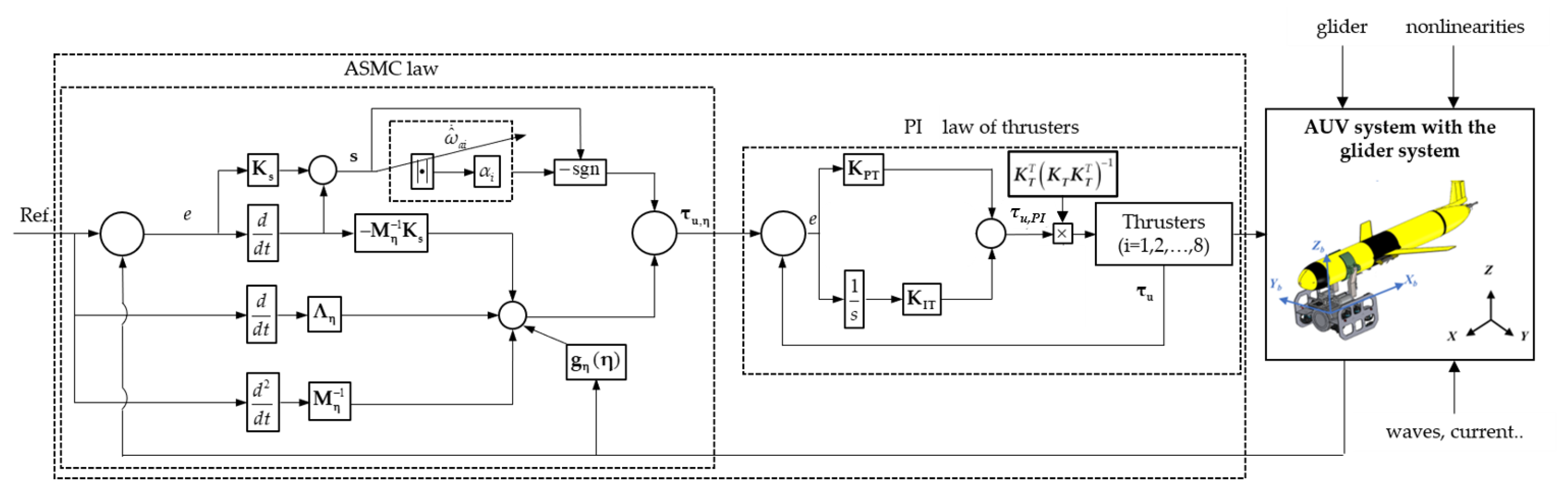
The schematic drawing of the proposed control system is depicted in Figure 6 below.

5. Simulation Results and Discussion

5.1. Simulation Setup

In this simulation study, we examine the motion control performance of the system. The simulation scenario is illustrated in Figure 7 and consists of the first and final stages of the recovery process. In the approaching stage, the ROV is deployed from the mother ship or operating station on the water surface. It dives into the water and then tracks a curvature trajectory to the below the glider. The glider is located at ${\left[\begin{array}{ccc}8& 6& 0\end{array}\right]}^T\left[\mathrm{m}\right]$ with respect to the initial location of the ROV. This stage consumes 80 [s] to finish. In a completed process, the ROV then performs the capturing stage, which is fundamentally a tracking task in a similar manner to the previous stage. Thus, we neglect it in the simulation. In the final stage, the ROV retrieves the glider back. The retrieving path can be simply a straight line since there is no concern about colliding with the glider as in the capturing stage. In other words, the desired trajectory in the simulation is given by:

$${\eta }_d\left(t\right)=\{\begin{array}{l}\frac{x^2}{25}+\frac{y^2}{25}+\frac{z^2}{r_d^2}=1\hspace{1em}\mathrm{if}\hspace{0.17em}t\le 80\hspace{0.17em}\hspace{0.17em}[s],\\ y=\frac{4}{3}x,\hspace{0.17em}z=0\hspace{1em}\hspace{0.17em}\hspace{0.17em}\hspace{0.17em}\hspace{0.17em}\hspace{0.17em}\hspace{0.17em}\hspace{0.17em}\mathrm{otherwise}\end{array}$$

(25)

The physical parameters of ROV in this simulation are given in

Table 1. The hydrodynamic parameters.

$\begin{array}{l}{X}_u=-72\hspace{0.17em}\mathrm{kg}{.\mathrm{s}}^{-1}\\ Y_v=-77\hspace{0.17em}\hspace{0.17em}\mathrm{kg}{.\mathrm{s}}^{-1} \\ Z_w=-95\hspace{0.17em}\mathrm{kg}{.\mathrm{s}}^{-1}\\ K_p=-40\hspace{0.17em}\hspace{0.17em}\mathrm{kg}.\mathrm{m}{.\mathrm{s}}^{-1}\\ M_q=-30\hspace{0.17em}\mathrm{kg}.\mathrm{m}{.\mathrm{s}}^{-1}\\ N_r=-30\hspace{0.17em}\mathrm{kg}.\mathrm{m}{.\mathrm{s}}^{-1}\end{array}$

$\begin{array}{l}{X}_{\dot{u}}=-29\hspace{0.17em}\mathrm{kg}\\ Y_{\dot{v}}=-30\hspace{0.17em}\hspace{0.17em}\mathrm{kg} \\ Z_{\dot{w}}=-90\hspace{0.17em}\mathrm{kg}\\ K_{\dot{p}}=-5.2\hspace{0.17em}\mathrm{kg}.\mathrm{m}\\ M_{\dot{q}}=-7.2\hspace{0.17em}\mathrm{kg}.\mathrm{m}\\ N_{\dot{r}}=-3.3\hspace{0.17em}\mathrm{kg}.\mathrm{m}\end{array}$

$\begin{array}{l}{X}_{u\left|u\right|}=0\hspace{0.17em}\mathrm{kg}{.\mathrm{m}}^{-1}\\ Y_{v\left|v\right|}=0\hspace{0.17em}\hspace{0.17em}\hspace{0.17em}\mathrm{kg}{.\mathrm{m}}^{-1} \\ Z_{w\left|w\right|}=0\hspace{0.17em}\mathrm{kg}{.\mathrm{m}}^{-1}\\ K_{p\left|p\right|}=0\hspace{0.17em}\hspace{0.17em}\mathrm{kg}{.\mathrm{m}}^{-1}\\ M_{q\left|q\right|}=0\hspace{0.17em}\mathrm{kg}{.\mathrm{m}}^{-1}\\ N_{r\left|r\right|}=0\hspace{0.17em}\hspace{0.17em}\mathrm{kg}{.\mathrm{m}}^{-1}\end{array}$

,

Table 2. The moments of inertia.

$\begin{array}{l}{I}_{xx}=1.32\hspace{0.17em}\mathrm{kg}{.\mathrm{m}}^2\\ I_{yy}=2.08\hspace{0.17em}\mathrm{kg}{.\mathrm{m}}^2\\ I_{zz}=2.32\hspace{0.17em}\mathrm{kg}{.\mathrm{m}}^2\end{array}$

$\begin{array}{l}{I}_{xy}=I_{xz}=0\hspace{0.17em}\mathrm{kg}{.\mathrm{m}}^2\\ I_{yx}=I_{yz}=0\hspace{0.17em}\mathrm{kg}{.\mathrm{m}}^2\\ I_{zx}=I_{zy}=0\hspace{0.17em}\mathrm{kg}{.\mathrm{m}}^2\end{array}$

,

Table 3. The center of gravity and buoyancy.

$\begin{array}{l}{x}_G=0\hspace{0.17em}\mathrm{m}\\ y_G=0\hspace{0.17em}\mathrm{m}\\ z_G=0\hspace{0.17em}\mathrm{m}\end{array}$

$\begin{array}{l}{x}_B=0\hspace{0.17em}\mathrm{m}\\ y_B=0\hspace{0.17em}\mathrm{m}\\ z_B=-0.05\hspace{0.17em}\mathrm{m}\end{array}$

,

Table 4. The underwater vehicles’ parameters.

$\begin{array}{l}\rho =1028.48\hspace{0.17em}\mathrm{kg}{.\mathrm{m}}^3\\ \nabla =0.09577\hspace{0.17em}{\mathrm{m}}^3\\ g=9.81\hspace{0.17em}\mathrm{m}{.\mathrm{s}}^{-2}\end{array}$

and

Table 5. The thrusters’ configuration parameters.

$\begin{array}{l}\delta =\frac{\pi }{4}\hspace{0.17em}\mathrm{rad}\\ l_{x1}=0.5\hspace{0.17em}\mathrm{m}\\ l_{y1}=0.5\hspace{0.17em}\mathrm{m}\\ l_{z1}=0.2\hspace{0.17em}\mathrm{m}\end{array}$

$\begin{array}{l}{l}_{x2}=0.15\hspace{0.17em}\mathrm{m}\\ l_{y2}=0.5\hspace{0.17em}\mathrm{m}\\ l_{z2}=0.2\hspace{0.17em}\mathrm{m}\end{array}$

and referred to in [35]. The parameters of the thruster models are experimentally obtained in [29] and shown in

Table 6. The parameters of the thruster hydrodynamic linear models.

$\begin{array}{l}{k}_1=13.66{\left[1\hspace{0.17em}\hspace{0.17em}\hspace{0.17em}1\hspace{0.17em}\hspace{0.17em}\hspace{0.17em}1\hspace{0.17em}\hspace{0.17em}\hspace{0.17em}1\hspace{0.17em}\hspace{0.17em}\hspace{0.17em}1\hspace{0.17em}\hspace{0.17em}\hspace{0.17em}1\right]}^T\hspace{1em}\hspace{1em}{\mathrm{s}}^{-1}\\ k_2=1856{\left[1\hspace{0.17em}\hspace{0.17em}\hspace{0.17em}1\hspace{0.17em}\hspace{0.17em}\hspace{0.17em}1\hspace{0.17em}\hspace{0.17em}\hspace{0.17em}1\hspace{0.17em}\hspace{0.17em}\hspace{0.17em}1\hspace{0.17em}\hspace{0.17em}\hspace{0.17em}1\right]}^T\hspace{1em}\hspace{1em}{\left(\mathrm{N}.\mathrm{m}{.\mathrm{s}}^2\right)}^{-1}\\ k_3=117.97{\left[1\hspace{0.17em}\hspace{0.17em}\hspace{0.17em}1\hspace{0.17em}\hspace{0.17em}\hspace{0.17em}1\hspace{0.17em}\hspace{0.17em}\hspace{0.17em}1\hspace{0.17em}\hspace{0.17em}\hspace{0.17em}1\hspace{0.17em}\hspace{0.17em}\hspace{0.17em}1\right]}^T\hspace{1em}\hspace{0.17em}\mathrm{m}{\left(\mathrm{N}{.\mathrm{s}}^2\right)}^{-1}\\ k_4=1.102{\left[1\hspace{0.17em}\hspace{0.17em}\hspace{0.17em}1\hspace{0.17em}\hspace{0.17em}\hspace{0.17em}1\hspace{0.17em}\hspace{0.17em}\hspace{0.17em}1\hspace{0.17em}\hspace{0.17em}\hspace{0.17em}1\hspace{0.17em}\hspace{0.17em}\hspace{0.17em}1\right]}^T\hspace{1em}\hspace{0.17em}\hspace{0.17em}\hspace{0.17em}{\mathrm{s}}^{-1}\\ k_5=0.01232{\left[1\hspace{0.17em}\hspace{0.17em}\hspace{0.17em}1\hspace{0.17em}\hspace{0.17em}\hspace{0.17em}1\hspace{0.17em}\hspace{0.17em}\hspace{0.17em}1\hspace{0.17em}\hspace{0.17em}\hspace{0.17em}1\hspace{0.17em}\hspace{0.17em}\hspace{0.17em}1\right]}^T\hspace{0.17em}\hspace{0.17em}\hspace{0.17em}\mathrm{m}{\left(\mathrm{N}{.\mathrm{s}}^2\right)}^{-1}\end{array}$

$\begin{array}{l}{c}_n^T=0.001467{\left[1\hspace{0.17em}\hspace{0.17em}\hspace{0.17em}1\hspace{0.17em}\hspace{0.17em}\hspace{0.17em}1\hspace{0.17em}\hspace{0.17em}\hspace{0.17em}1\hspace{0.17em}\hspace{0.17em}\hspace{0.17em}1\hspace{0.17em}\hspace{0.17em}\hspace{0.17em}1\right]}^T\hspace{1em}\hspace{0.17em}\hspace{0.17em}\hspace{0.17em}\mathrm{N}{.\mathrm{s}}^2\\ c_{n\upsilon }^T=0.4146{\left[1\hspace{0.17em}\hspace{0.17em}\hspace{0.17em}1\hspace{0.17em}\hspace{0.17em}\hspace{0.17em}1\hspace{0.17em}\hspace{0.17em}\hspace{0.17em}1\hspace{0.17em}\hspace{0.17em}\hspace{0.17em}1\hspace{0.17em}\hspace{0.17em}\hspace{0.17em}1\right]}^T\hspace{1em}\hspace{0.17em}\hspace{0.17em}\hspace{0.17em}\hspace{0.17em}\hspace{0.17em}\hspace{0.17em}\mathrm{N}{.\mathrm{s}}^2{.\mathrm{m}}^{-1}\\ c_n^Q=2.804\times {10}^{-6}{\left[1\hspace{0.17em}\hspace{0.17em}\hspace{0.17em}1\hspace{0.17em}\hspace{0.17em}\hspace{0.17em}1\hspace{0.17em}\hspace{0.17em}\hspace{0.17em}1\hspace{0.17em}\hspace{0.17em}\hspace{0.17em}1\hspace{0.17em}\hspace{0.17em}\hspace{0.17em}1\right]}^T\hspace{0.17em}\hspace{0.17em}\hspace{0.17em}\mathrm{N}{.\mathrm{s}}^2{.\mathrm{m}}^{-2}\\ c_{n\upsilon }^Q=1.296\times {10}^{-11}{\left[1\hspace{0.17em}\hspace{0.17em}\hspace{0.17em}1\hspace{0.17em}\hspace{0.17em}\hspace{0.17em}1\hspace{0.17em}\hspace{0.17em}\hspace{0.17em}1\hspace{0.17em}\hspace{0.17em}\hspace{0.17em}1\hspace{0.17em}\hspace{0.17em}\hspace{0.17em}1\right]}^T\mathrm{N}{.\mathrm{s}}^2\\ U=0.35{\left[1\hspace{0.17em}\hspace{0.17em}\hspace{0.17em}1\hspace{0.17em}\hspace{0.17em}\hspace{0.17em}1\hspace{0.17em}\hspace{0.17em}\hspace{0.17em}1\hspace{0.17em}\hspace{0.17em}\hspace{0.17em}1\hspace{0.17em}\hspace{0.17em}\hspace{0.17em}1\right]}^T\hspace{1em}\hspace{1em}\hspace{1em}\hspace{1em}\hspace{0.17em}\mathrm{m}{.\mathrm{s}}^{-1}\end{array}$

. The total effect of waves, wind, and ocean currents is defined through ${\theta }_{\upsilon C}={\left[0.15\hspace{0.17em}[\mathrm{N}]\hspace{0.17em}\hspace{0.17em}\hspace{0.17em}\hspace{0.17em}0.35\hspace{0.17em}[\mathrm{N}]\hspace{0.17em}\hspace{0.17em}\hspace{0.17em}0.8\hspace{0.17em}[\mathrm{N}]\hspace{0.17em}\hspace{0.17em}\hspace{0.17em}0.02\hspace{0.17em}[\mathrm{Nm}]\hspace{0.17em}\hspace{0.17em}\hspace{0.17em}0.05\hspace{0.17em}[\mathrm{Nm}]\hspace{0.17em}\hspace{0.17em}\hspace{0.17em}0.07\hspace{0.17em}[\mathrm{Nm}]\right]}^T$. The influence of the retrieval glider is treated as additive resistance forces and moments in the latter part of the simulation. In this paper, we assume the effect of the glider is a constant ${\tau }_G={\left[20.3\hspace{0.17em}[\mathrm{N}]\hspace{0.17em}\hspace{0.17em}\hspace{0.17em}20.3\hspace{0.17em}[\mathrm{N}]\hspace{0.17em}\hspace{0.17em}\hspace{0.17em}20.3\hspace{0.17em}[\mathrm{N}]\hspace{0.17em}\hspace{0.17em}\hspace{0.17em}5.6\hspace{0.17em}[\mathrm{Nm}]\hspace{0.17em}\hspace{0.17em}\hspace{0.17em}7.6\hspace{0.17em}[\mathrm{Nm}]\hspace{0.17em}\hspace{0.17em}\hspace{0.17em}10.3\hspace{0.17em}[\mathrm{Nm}]\right]}^T$. The other disturbances are also added to the scenario to validate the robustness of the control system. They are given by:

$${\tau }_d={\left[2.3\sin 0.4t\hspace{0.17em}[\mathrm{N}]\hspace{0.17em}\hspace{0.17em}\hspace{0.17em}\hspace{0.17em}1.5\sin 0.8t\hspace{0.17em}[\mathrm{N}]\hspace{0.17em}\hspace{0.17em}\hspace{0.17em}\hspace{0.17em}4\sin 0.7t\hspace{0.17em}[\mathrm{N}]\hspace{0.17em}\hspace{0.17em}\hspace{0.17em}\hspace{0.17em}0.15\sin 0.1t\hspace{0.17em}[\mathrm{Nm}]\hspace{0.17em}\hspace{0.17em}\hspace{0.17em}\hspace{0.17em}\hspace{0.17em}0.1\sin 0.4t\hspace{0.17em}[\mathrm{Nm}]\hspace{0.17em}\hspace{0.17em}\hspace{0.17em}\hspace{0.17em}\hspace{0.17em}0.2\sin 0.5t\hspace{0.17em}[\mathrm{Nm}]\right]}^T$$

(26)

For the sake of validation, a cascade PID-PI control system is taken into comparison with our proposed ASMC-PI. Their parameters are listed in

Table 7. The controllers’ gains.

Outer loop	ASMC	$\begin{array}{c}{K}_s=diag\left(11.50,\hspace{0.17em}\hspace{0.17em}6.81,\hspace{0.17em}\hspace{0.17em}7.52,\hspace{0.17em}\hspace{0.17em}16.51,\hspace{0.17em}\hspace{0.17em}11.52,\hspace{0.17em}\hspace{0.17em}14.11\right),\\ \alpha =diag\left(28.51,\hspace{0.17em}\hspace{0.17em}32.18,\hspace{0.17em}\hspace{0.17em}5.27,\hspace{0.17em}\hspace{0.17em}7.12,\hspace{0.17em}\hspace{0.17em}8.32,\hspace{0.17em}\hspace{0.17em}14.12\right)\end{array}$
	PID	$\begin{array}{c}{K}_P=diag\left(145,\hspace{0.17em}\hspace{0.17em}200,\hspace{0.17em}\hspace{0.17em}183,\hspace{0.17em}\hspace{0.17em}84,\hspace{0.17em}\hspace{0.17em}40,\hspace{0.17em}\hspace{0.17em}50\right),\\ K_I=diag\left(140,\hspace{0.17em}\hspace{0.17em}230,\hspace{0.17em}\hspace{0.17em}180,\hspace{0.17em}\hspace{0.17em}32,\hspace{0.17em}\hspace{0.17em}25,\hspace{0.17em}\hspace{0.17em}25\right),\\ K_D=diag\left(106,\hspace{0.17em}\hspace{0.17em}170,\hspace{0.17em}\hspace{0.17em}350,\hspace{0.17em}\hspace{0.17em}82,\hspace{0.17em}\hspace{0.17em}74,\hspace{0.17em}\hspace{0.17em}60\right)\end{array}$
Inner loop	PI	$\begin{array}{c}{K}_{PT}=diag\left(0.85,\hspace{0.17em}\hspace{0.17em}0.99,\hspace{0.17em}\hspace{0.17em}0.6,\hspace{0.17em}\hspace{0.17em}0.15,\hspace{0.17em}\hspace{0.17em}0.1,\hspace{0.17em}\hspace{0.17em}0.89\right),\\ K_{IT}=diag\left(15,\hspace{0.17em}\hspace{0.17em}5.1,\hspace{0.17em}\hspace{0.17em}10,\hspace{0.17em}\hspace{0.17em}15,\hspace{0.17em}\hspace{0.17em}10,\hspace{0.17em}\hspace{0.17em}16.1\right)\end{array}$

.

5.2. Motion Performance in the Approaching Stage

The tracking performance of the ROV in 3D geometry is illustrated in Figure 8 and the tracking error in each direction with respect to time is shown in Figure 9. Both controllers are able to maneuver the ROV following the desired trajectory, but the proposed cascade ASMC-PI controller performs better. Although the proposed controller seems to give a larger fluctuation than the PID controller at the beginning, the tracking errors in Figure 9 show that only the motion in the z-direction is the case. The deviation in the z-direction motion quickly converges in 20 [s] and remains in a neighbor of zero after that. In comparison, the PID-PI controlled system had a smaller tracking error in this direction at the beginning. However, it is unable to compensate effectively for the error and results in fluctuation in the whole period. Better performances of the proposed control system are easily seen in every other direction. The voltage inputs in Figure 10 show that the ASMC-PI controller quickly adjusts the operation of each thruster such that high-precision tracking is achieved. Especially when the ROV reaches the end of the first stage, it is close to the glider. Thus, deviation from the tracking trajectory may lead to a collision between the two vehicles.

5.3. Motion Performance in the Retrieving Stage

The motion performance in the retrieving stage is represented in the same manner as the previous stage. The tracking trajectory, tracking errors and voltage inputs are respectively shown in Figure 11, Figure 12 and Figure 13. Due to the resistant force and moment of the glider, the motion performance is worse than in the first two stages. For example, the roll and pitch of the ROV controlled by the proposed ASMC-PI cannot converge completely. Fortunately, the stable motion of the ROV is still maintained. Meanwhile, the effects of the glider on the ROV’s motion are significant with the comparative PID-PI controller. It is also worth noting that the requirement of precision tracking is not as critical as in the first two stages. Therefore, the ROV has proved its ability for the glider recovery mission, and the proposed ASMC-PI control system has demonstrated its superiority.

6. Conclusions

In this study, a novel recovery process has been proposed for an underwater glider by using ROV and a motion control system. The ROV is equipped with instruments and capturing mechanisms to perform three successive tasks: approaching, capturing, and retrieving the glider. The cascade ASMC-PI controller has been designed such that a safe and effective recovery is achieved. In order to validate the proposed system, the simulations were conducted in the first and final stages of the recovery process. The simulation results show that the proposed system achieves high motion performance in the former stage and maintains a robust operation in the latter. In comparison with a cascade PID-PI control system, the proposed system demonstrated its superiority in the recovery process.

For future works, the specifications of the ROV and the glider will shortly be finalized. The experimental system will be fabricated, and experimental studies will be conducted for further evaluation.