

Hydrodynamic Behaviour of a Floating Polygonal Platform Centrally Placed within a Polygonal Ring Structure under Wave Action


Abstract
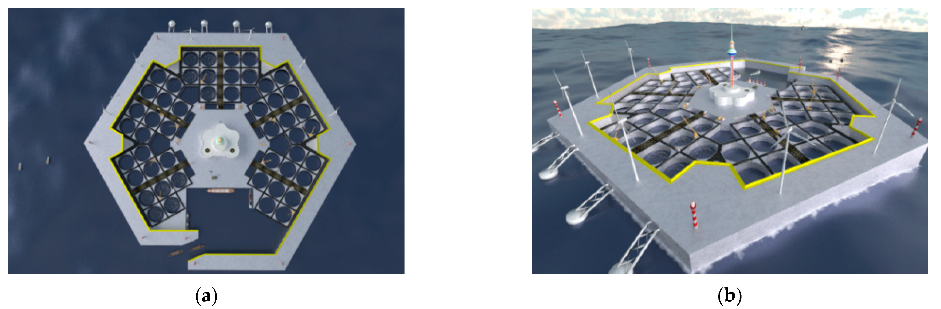
:1. Introduction
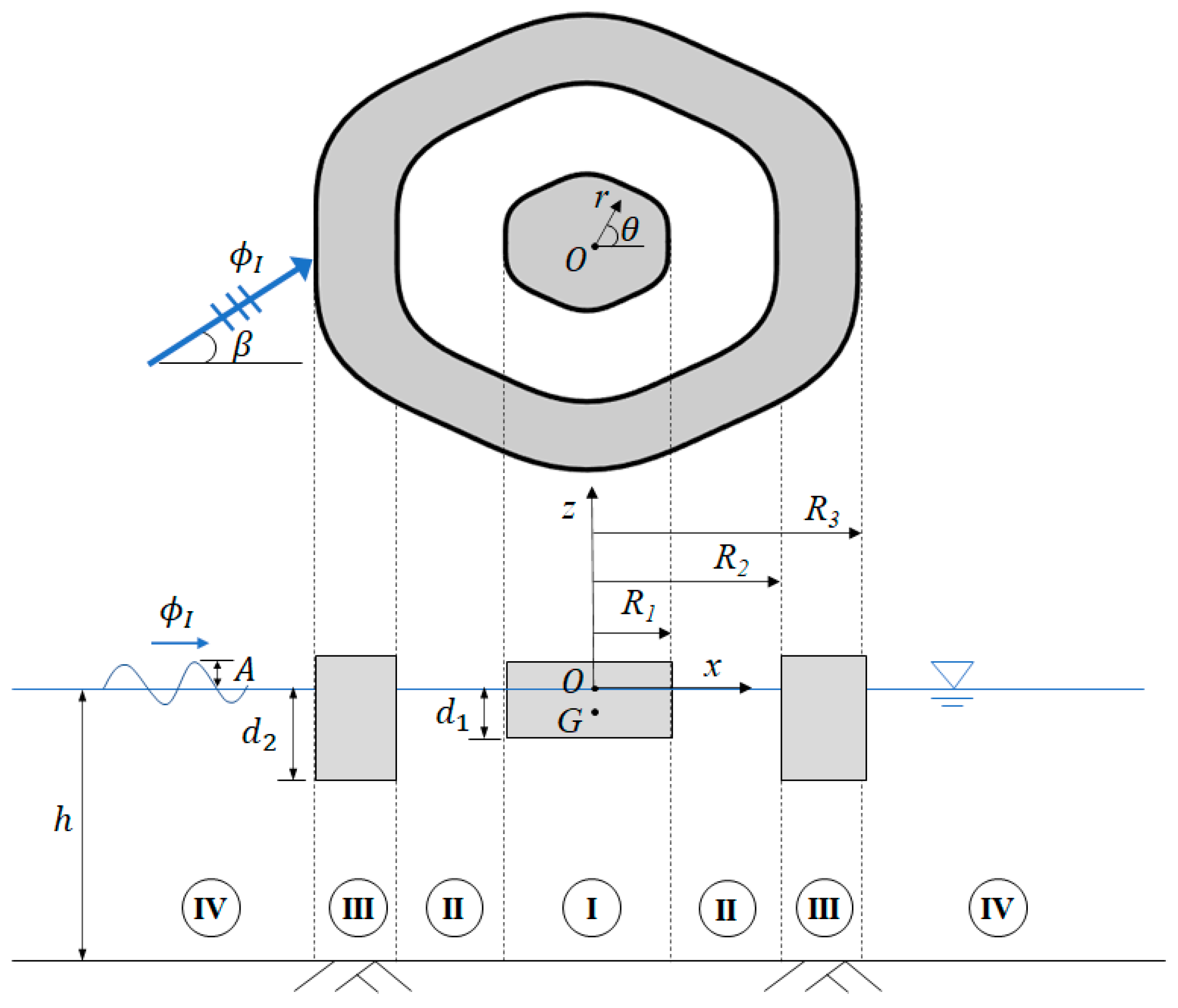
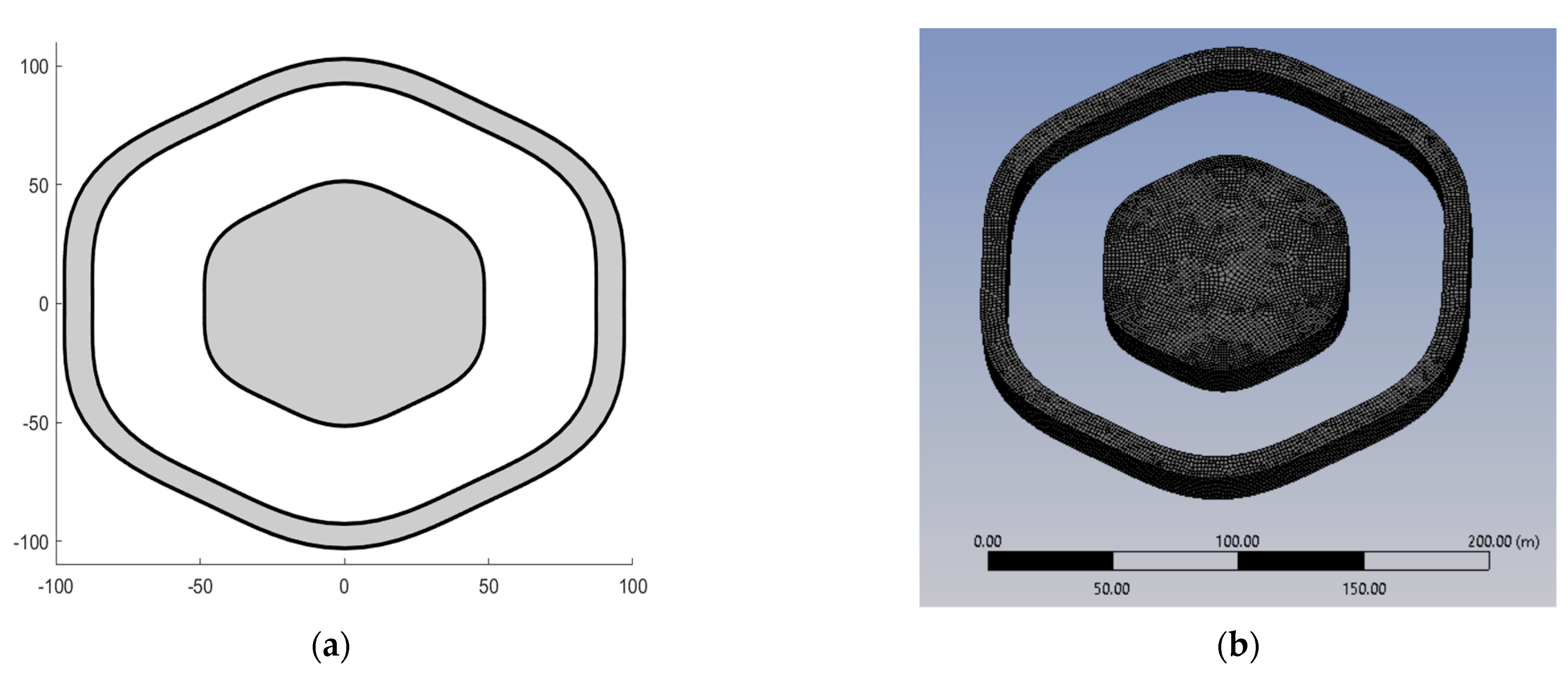
2. Problem Definition
3. Governing Equation and Boundary Conditions
4. Solutions for Diffracted and Radiated Potentials
5. Determination of Wave Exciting Force
6. Determination of Radiation Forces
7. Motion Responses of Floating Ring Structure
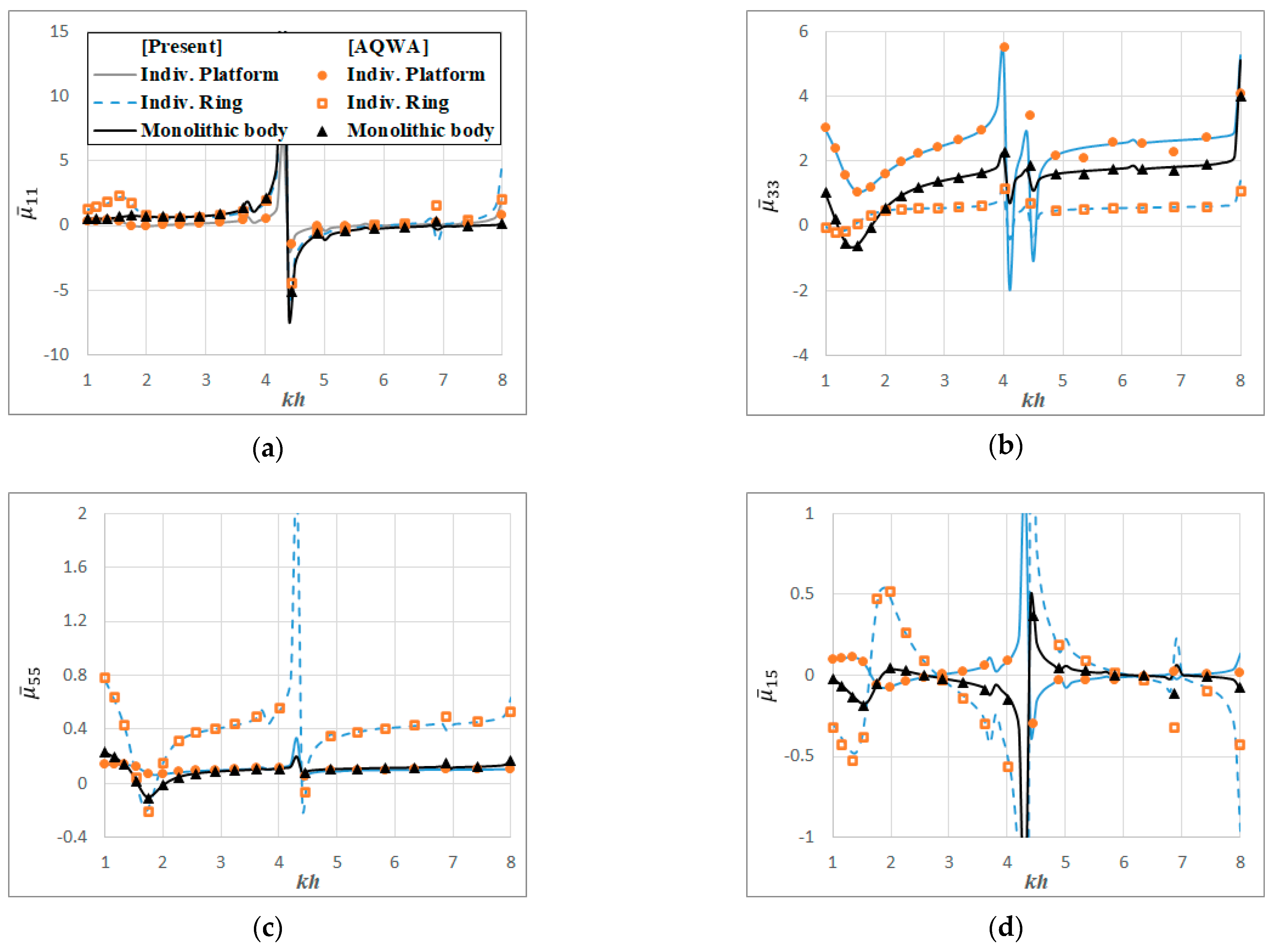
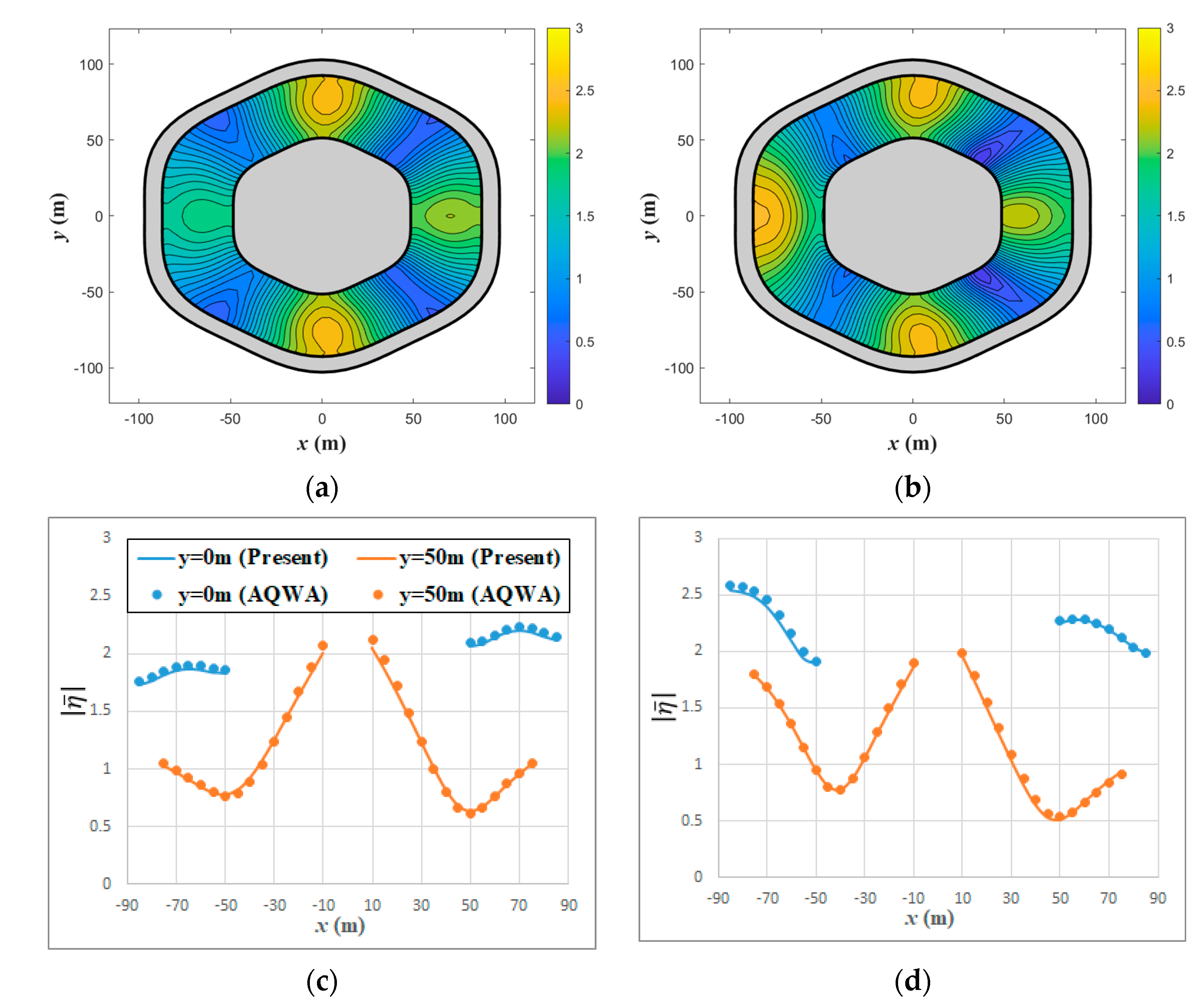
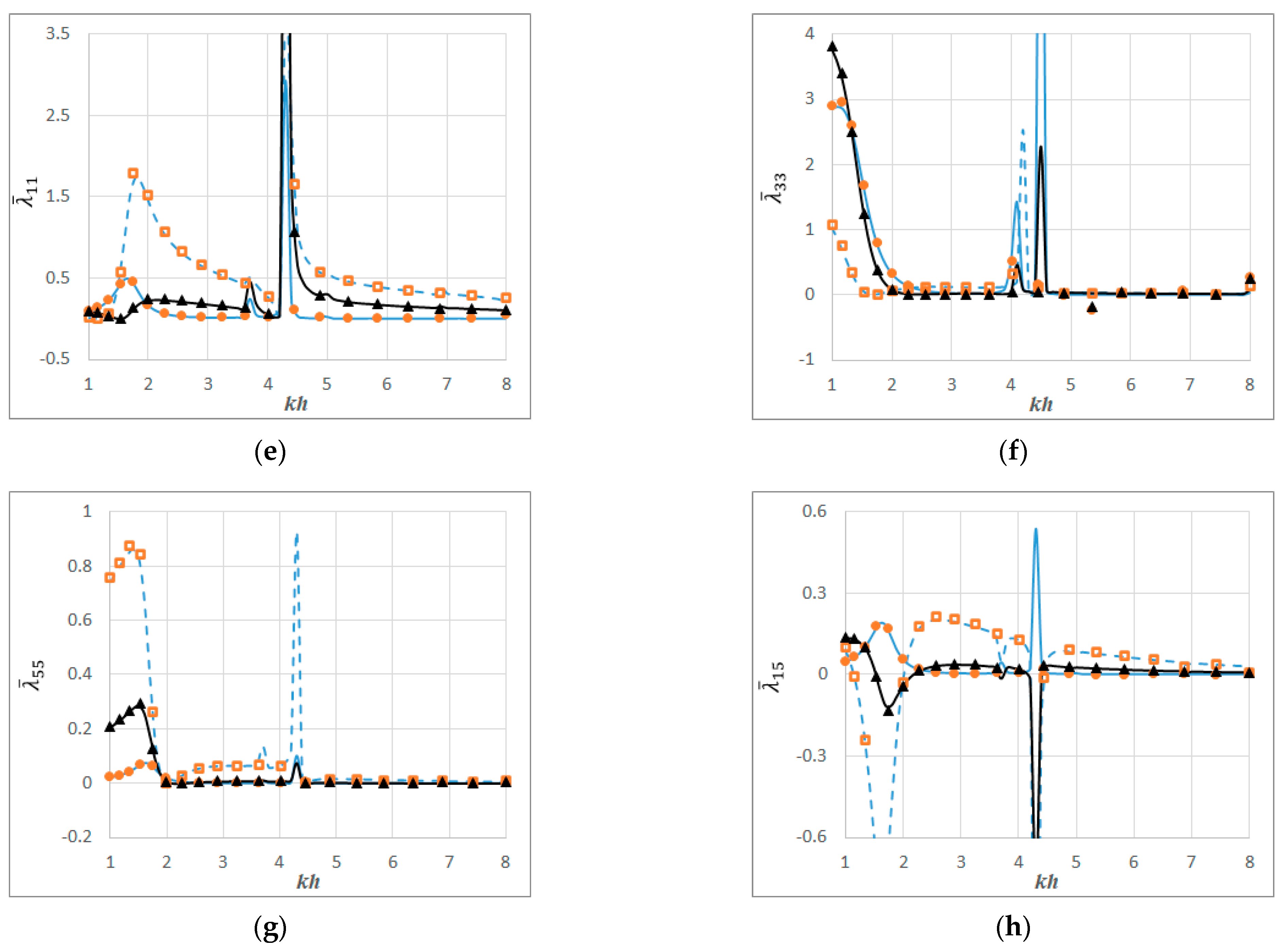
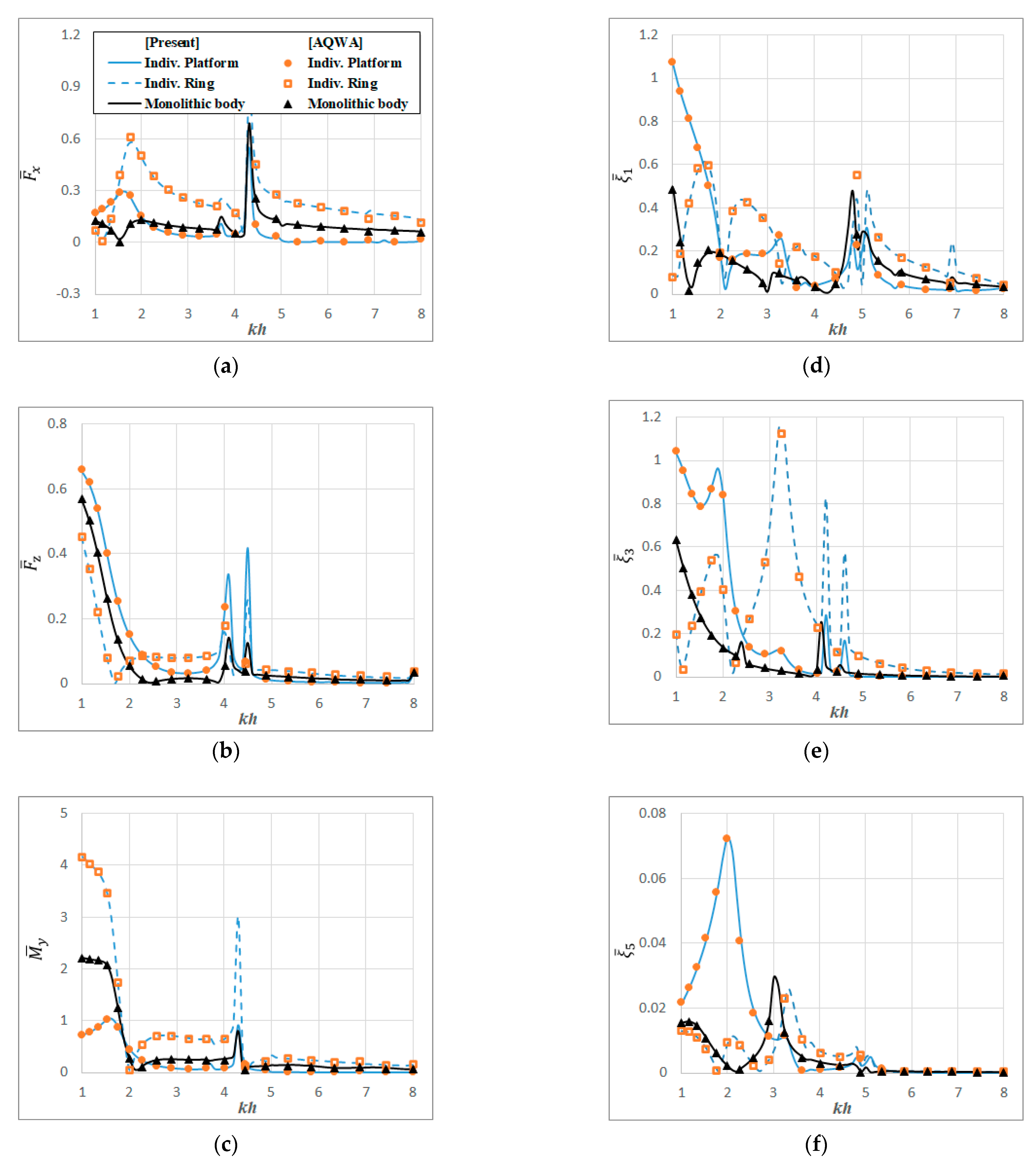
8. Verification of Semi-Analytical Approach and Computer Code
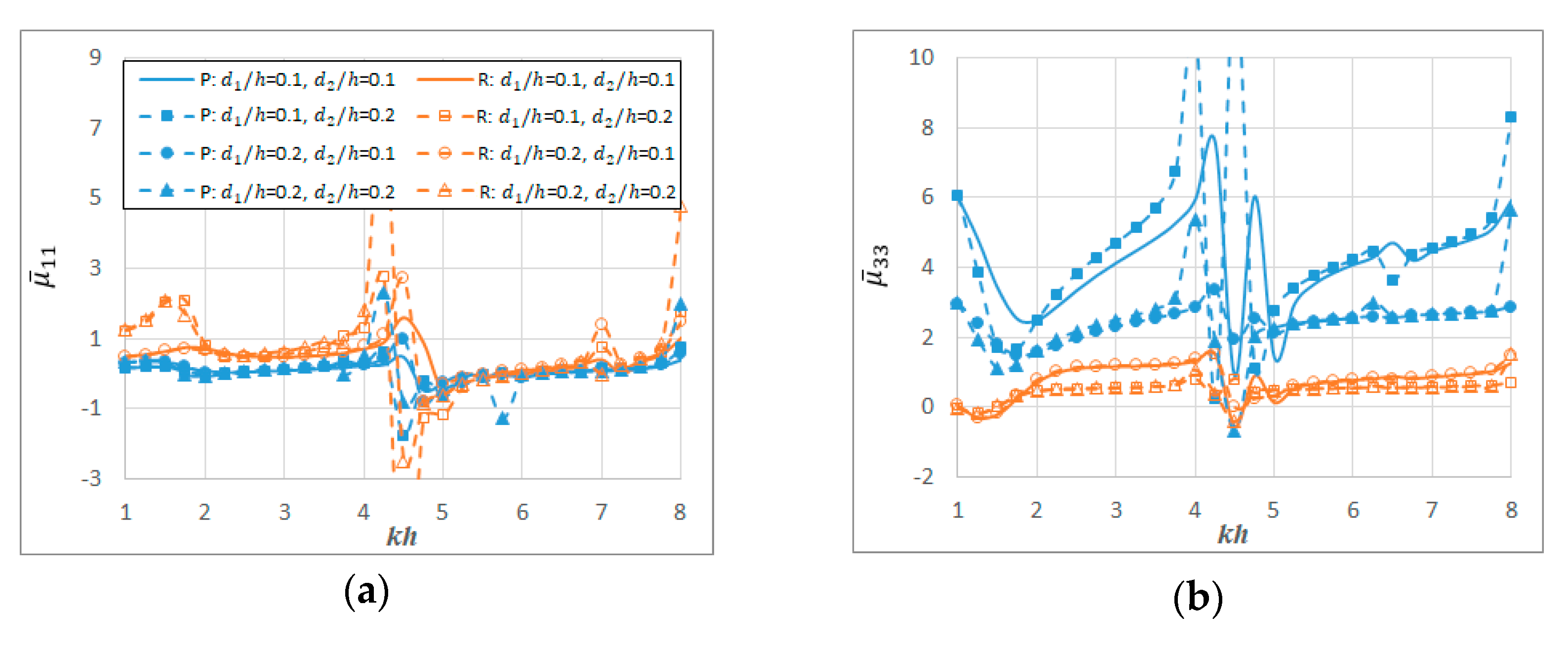
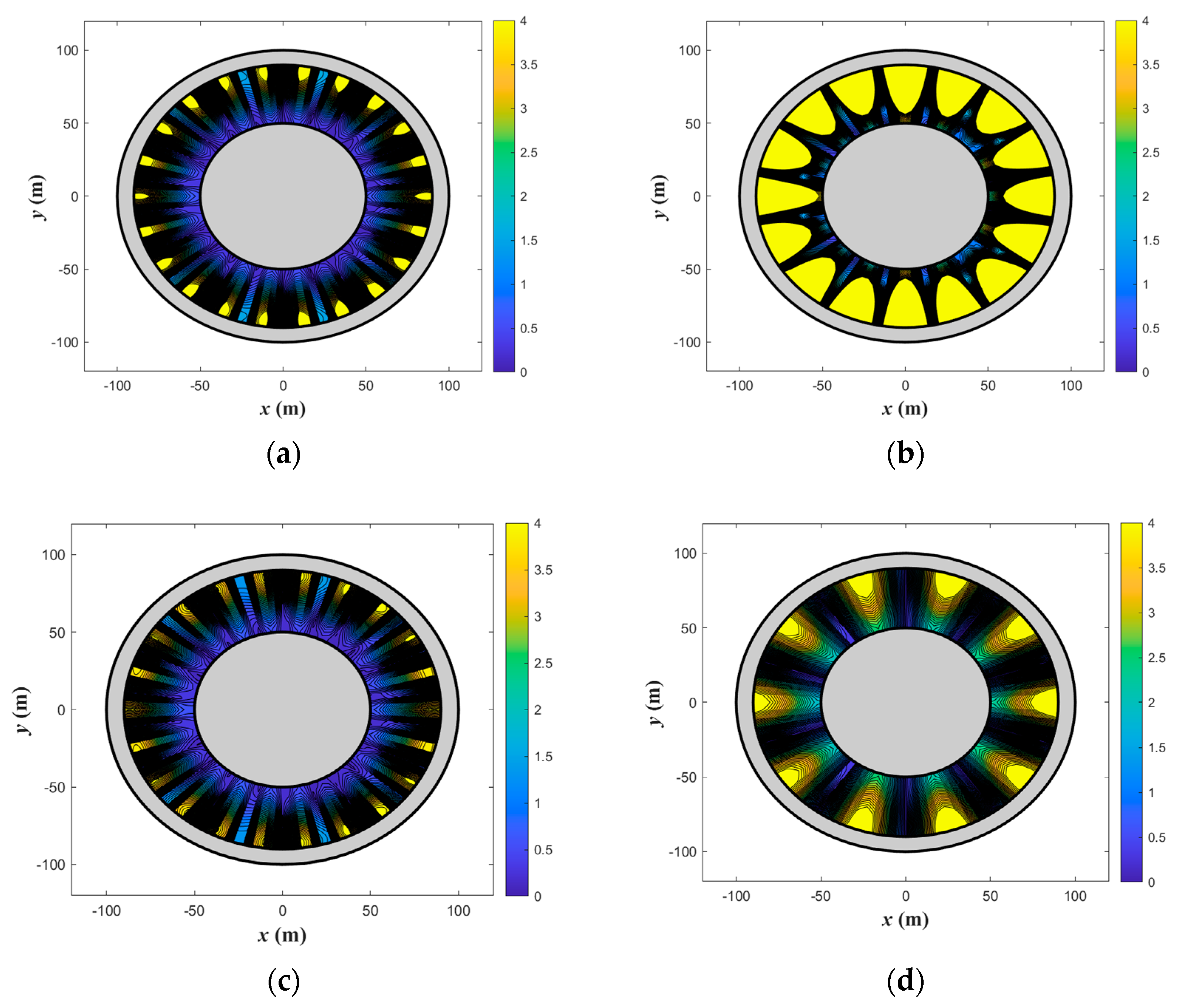
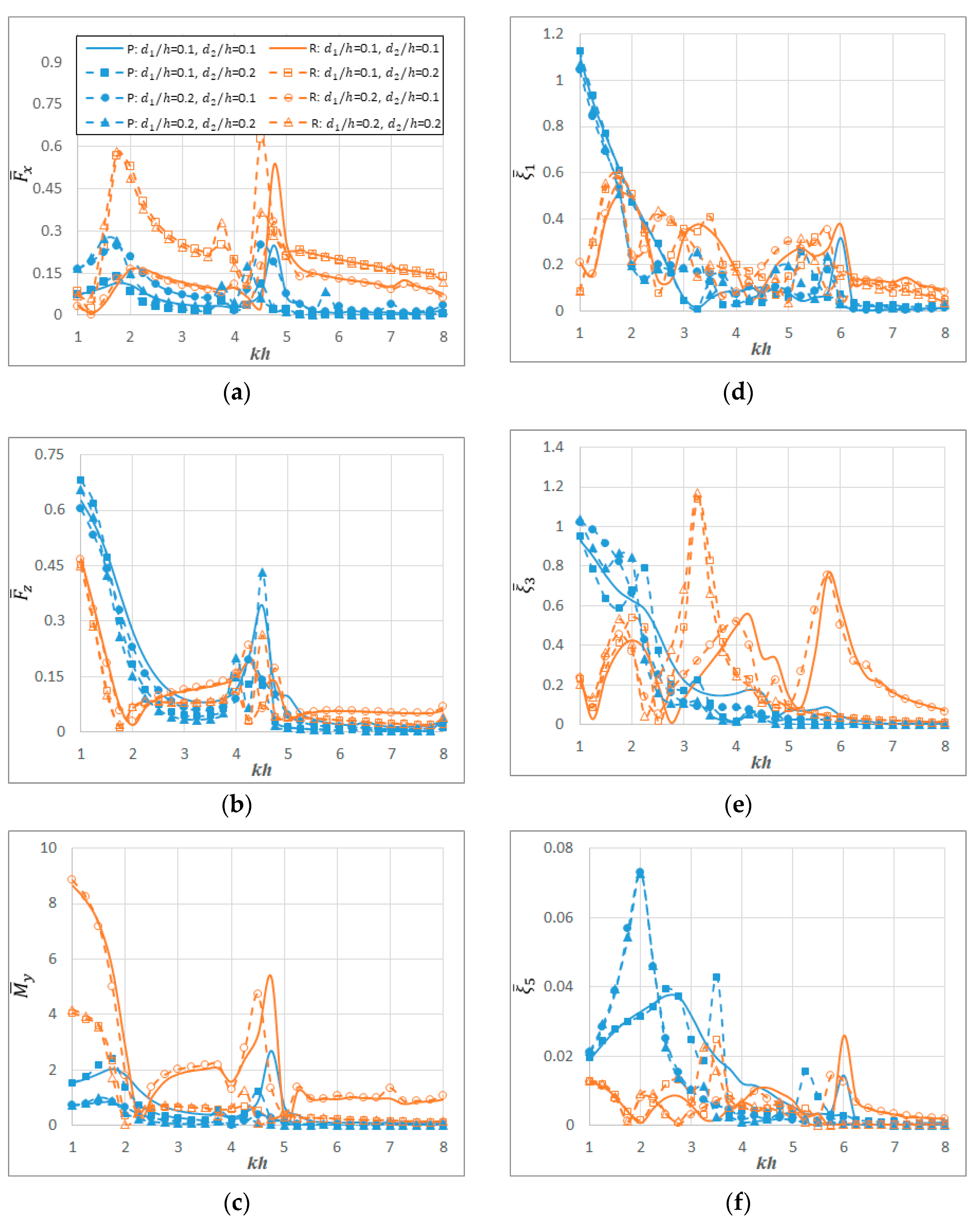
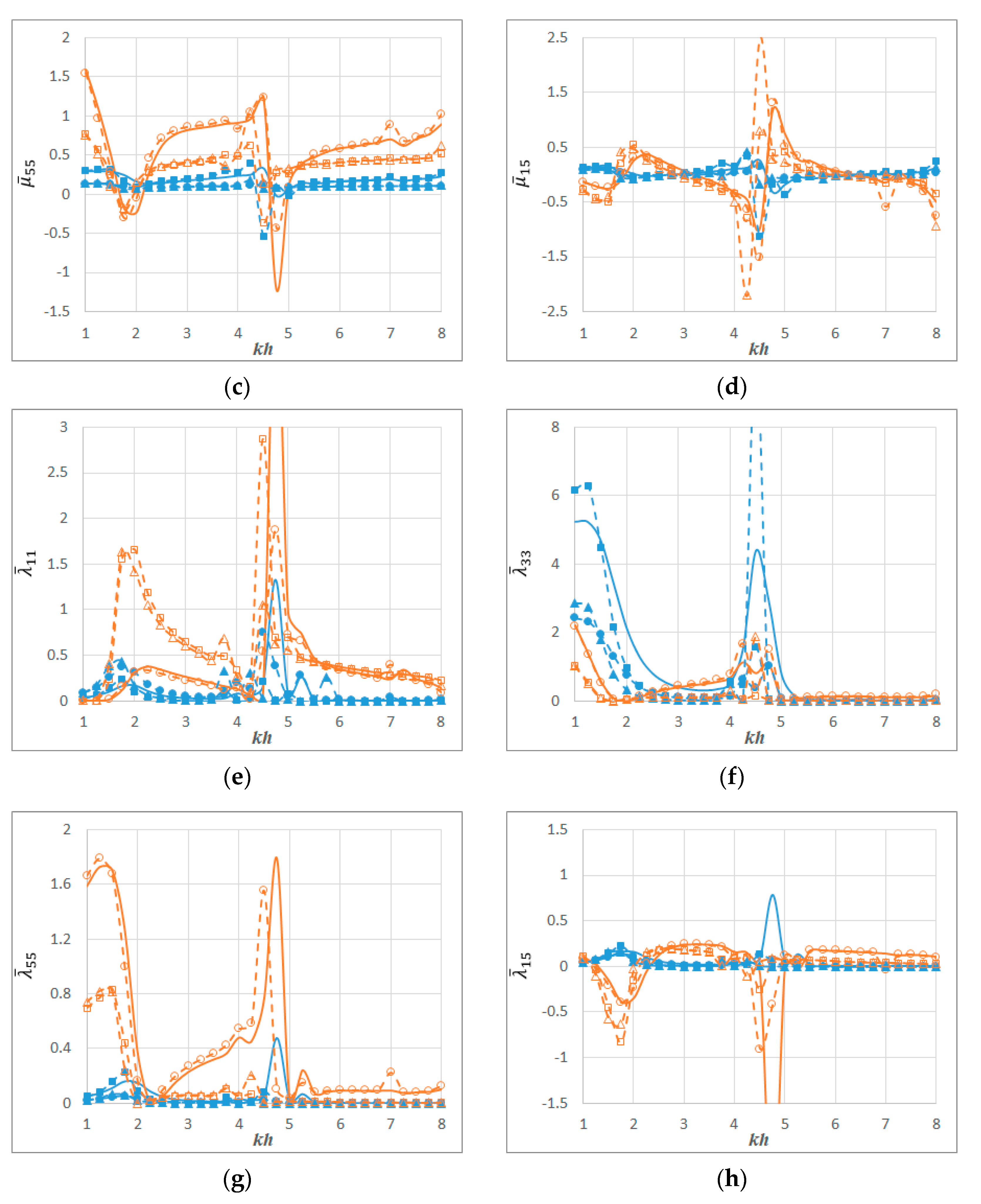
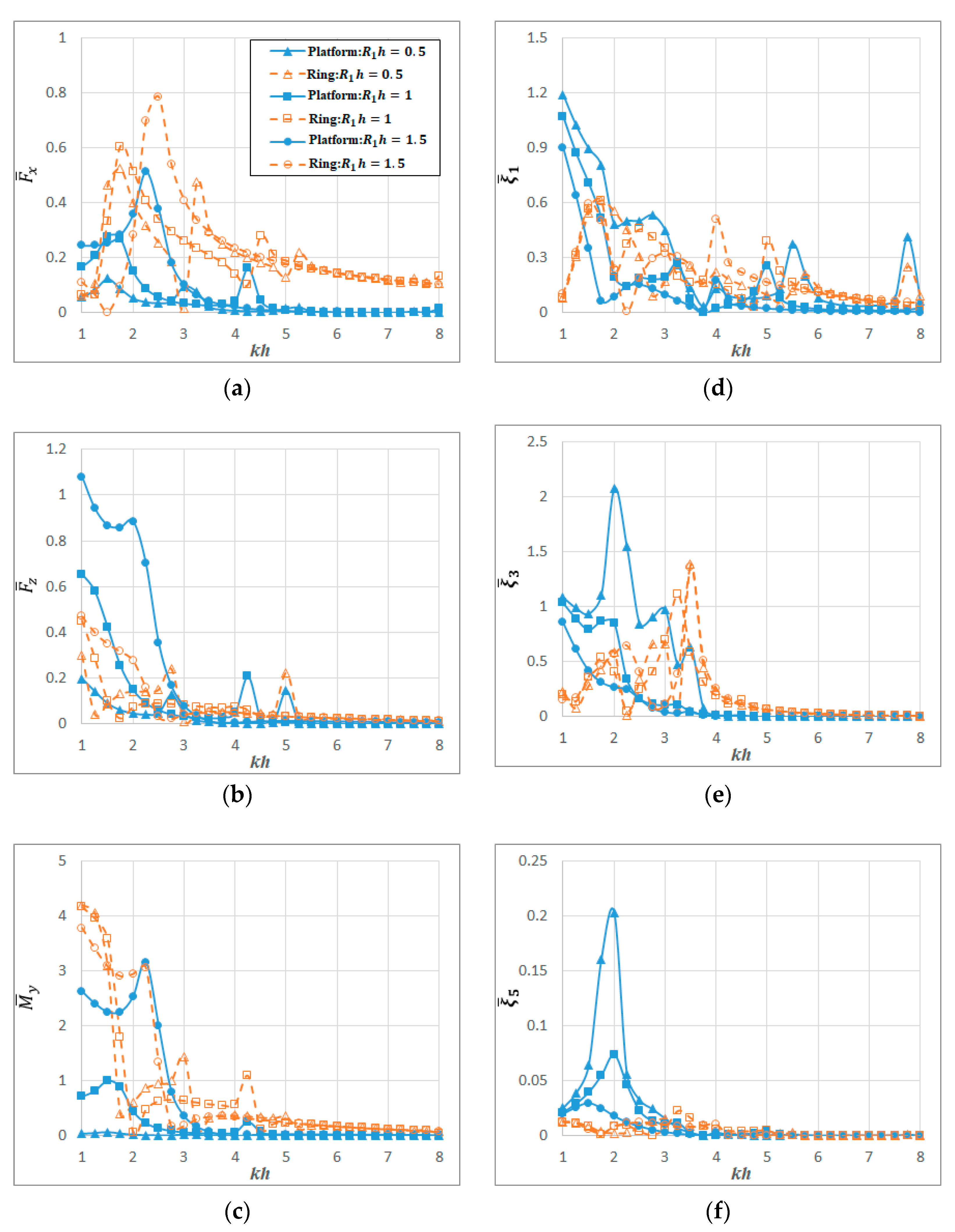
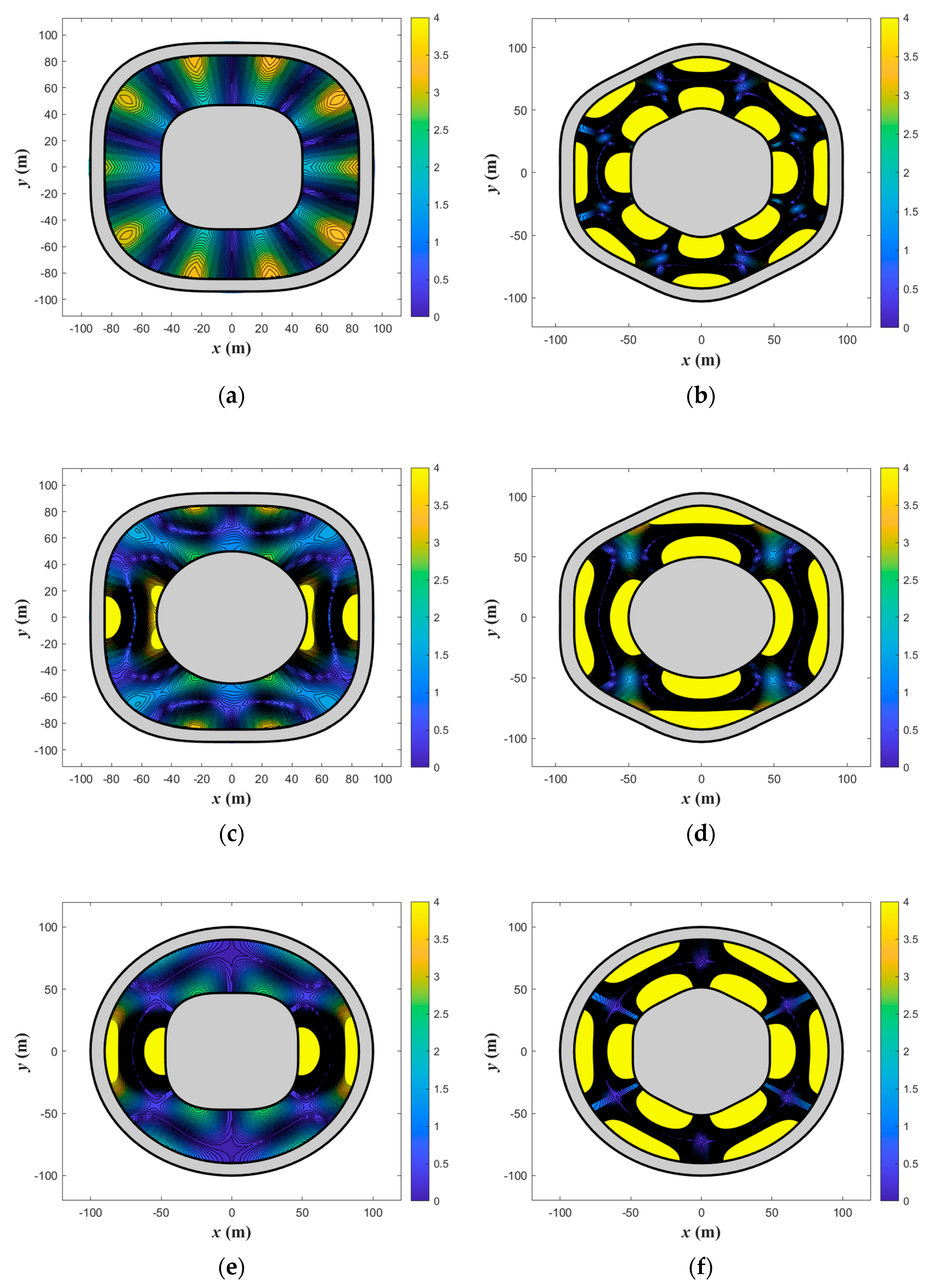
9. Results and Discussion
10. Concluding Remarks
Author Contributions
Funding
Institutional Review Board Statement
Informed Consent Statement
Data Availability Statement
Conflicts of Interest
Appendix A
Appendix B
Appendix C
References
- Wang, C.M.; Wang, B. Large Floating Structures; Springer: Singapore, 2015; Volume 3. [Google Scholar]
- Wang, C.M.; Lim, S.H.; Tay, Z.Y. WCFS2019: Proceedings of the the World Conference on Floating Solutions; Springer: Singapore, 2020. [Google Scholar]
- Piątek, Ł.; Lim, S.H.; Wang, C.M.; Graaf-van Dinther, R. WCFS2020: Proceedings of the the Second World Conference of Floating Solutions, Rotterdam; Springer: Singapore, 2022. [Google Scholar]
- Miloh, T. Wave loads on a floating solar pond. In The Proceedings, International Workshop on Ship and Platform Motions; Yeung, R.W., Ed.; University of California: Berkeley, CA, USA, 1983. [Google Scholar]
- Wang, C.M.; Chu, Y.I.; Park, J.C. Moving offshore for fish farming. J. Aquac. Mar. Biol. 2019, 8, 38–39. [Google Scholar] [CrossRef]
- McNown, J.S. 18. Waves and Seiche in Idealized Ports. In Proceedings of NBS Semicentennial Symposium on Gravity Waves Held at the NBS on June 18–20, 1951; National Bureau of Standards Circular 521: Washington, DC, USA, 1952; pp. 153–164. [Google Scholar]
- Miles, J.; Munk, W. Harbor paradox. J. Waterw. Harb. Div. 1961, 87, 111–132. [Google Scholar] [CrossRef]
- Garrett, C. Bottomless harbours. J. Fluid Mech. 1970, 43, 433–449. [Google Scholar] [CrossRef]
- Fernandes, A.C. Analysis of an Axisymmetric Pneumatic Buoy by Reciprocity Relations and a Ring-Source Method; Massachusetts Institute of Technology: Cambridge, MA, USA, 1983. [Google Scholar]
- Konispoliatis, D.; Mazarakos, T.; Mavrakos, S. Hydrodynamic analysis of three–unit arrays of floating annular oscillating–water–column wave energy converters. Appl. Ocean Res. 2016, 61, 42–64. [Google Scholar] [CrossRef]
- Mavrakos, S. Wave loads on a stationary floating bottomless cylindrical body with finite wall thickness. Appl. Ocean Res. 1985, 7, 213–224. [Google Scholar] [CrossRef]
- Mavrakos, S. Hydrodynamic coefficients for a thick-walled bottomless cylindrical body floating in water of finite depth. Ocean Eng. 1988, 15, 213–229. [Google Scholar] [CrossRef]
- Mavrakos, S.A.; Chatjigeorgiou, I.K. Second-order hydrodynamic effects on an arrangement of two concentric truncated vertical cylinders. J. Mar. Struct. 2009, 22, 545–575. [Google Scholar] [CrossRef]
- Mavrakos, S.A. Hydrodynamic coefficients in heave of two concentric surface-piercing truncated circular cylinders. Appl. Ocean Res. 2004, 26, 84–97. [Google Scholar] [CrossRef]
- Mavrakos, S.A. Hydrodynamic characteristics of two concentric surface–piercing. Mitochondrial Med. 2006, 221–228. [Google Scholar]
- Mavrakos, S.A.; Katsaounis, G.M.; Chatjigeorgiou, I.K. Performance characteristics of a tightly moored piston-like wave energy converter under first-and second-order wave loads. In International Conference on Offshore Mechanics and Arctic Engineering; AMSE: Estoril, Portugal, 2008; pp. 783–792. [Google Scholar]
- Wetmore, S.B.; Ramsden, H.D. CIDS: A Mobile Concrete Island Drilling System for Arctic Offshore Operations. Mar. Technol. SNAME News 1984, 21, 1–11. [Google Scholar] [CrossRef]
- Fishfarmexpert. FjordMAX Promises More Fish and Smaller Footprint. Available online: https://www.fishfarmingexpert.com/article/fjordmax-promises-more-fish-and-smaller-footprint/ (accessed on 25 July 2022).
- Wang, P.; Zhao, M.; Du, X.; Liu, J. Analytical solution for the short-crested wave diffraction by an elliptical cylinder. Eur. J. Mech.-B/Fluids 2019, 74, 399–409. [Google Scholar] [CrossRef]
- Park, J.C.; Wang, C.M. Hydrodynamic behaviour of floating polygonal platforms under wave action. J. Mar. Sci. Eng. 2021, 9, 923. [Google Scholar] [CrossRef]
- Park, J.C.; Wang, C. Hydrodynamic behaviour of floating polygonal ring structures under wave action. Ocean Eng. 2022, 249, 110195. [Google Scholar] [CrossRef]
- Mansour, A.M.; Williams, A.N.; Wang, K. The diffraction of linear waves by a uniform vertical cylinder with cosine-type radial perturbations. Ocean Eng. 2002, 29, 239–259. [Google Scholar] [CrossRef]
- Liu, J.; Guo, A.; Li, H. Analytical solution for the linear wave diffraction by a uniform vertical cylinder with an arbitrary smooth cross-section. Ocean Eng. 2016, 126, 163–175. [Google Scholar] [CrossRef]
- Liu, J.; Guo, A.; Fang, Q.; Li, H.; Hu, H.; Liu, P. Investigation of linear wave action around a truncated cylinder with non-circular cross section. J. Mar. Sci. Technol. 2018, 23, 866–876. [Google Scholar] [CrossRef]


| Polygonal Shapes |  Circle |  Triangle |  Square |  Pentagon |  Hexagon |
|---|---|---|---|---|---|
| Velocity Potential | Condition | Functions Used | Fourier Expansions | ||
|---|---|---|---|---|---|
| Incoming waves | |||||
| Incoming waves | |||||
| Outgoing waves | |||||
| Incoming waves | |||||
| Outgoing waves | |||||
| Outgoing waves | |||||
| N/A | Incident waves | ||||
| Derivative of Velocity Potential | Condition | Functions Used | Fourier Expansions | ||
|---|---|---|---|---|---|
| Incoming waves | |||||
| Incoming waves | |||||
| Outgoing waves | |||||
| Incoming waves | |||||
| Outgoing waves | |||||
| Outgoing waves | |||||
| N/A | Incident waves | ||||
Publisher’s Note: MDPI stays neutral with regard to jurisdictional claims in published maps and institutional affiliations. |
© 2022 by the authors. Licensee MDPI, Basel, Switzerland. This article is an open access article distributed under the terms and conditions of the Creative Commons Attribution (CC BY) license (https://creativecommons.org/licenses/by/4.0/).
Share and Cite
Park, J.C.; Wang, C.M. Hydrodynamic Behaviour of a Floating Polygonal Platform Centrally Placed within a Polygonal Ring Structure under Wave Action. J. Mar. Sci. Eng. 2022, 10, 1430. https://doi.org/10.3390/jmse10101430
Park JC, Wang CM. Hydrodynamic Behaviour of a Floating Polygonal Platform Centrally Placed within a Polygonal Ring Structure under Wave Action. Journal of Marine Science and Engineering. 2022; 10(10):1430. https://doi.org/10.3390/jmse10101430
Chicago/Turabian StylePark, Jeong Cheol, and Chien Ming Wang. 2022. "Hydrodynamic Behaviour of a Floating Polygonal Platform Centrally Placed within a Polygonal Ring Structure under Wave Action" Journal of Marine Science and Engineering 10, no. 10: 1430. https://doi.org/10.3390/jmse10101430
APA StylePark, J. C., & Wang, C. M. (2022). Hydrodynamic Behaviour of a Floating Polygonal Platform Centrally Placed within a Polygonal Ring Structure under Wave Action. Journal of Marine Science and Engineering, 10(10), 1430. https://doi.org/10.3390/jmse10101430