
The Numerical Simulation of a Submarine Based on a Dynamic Mesh Method

1
School of Ocean Engineering, Harbin Institute of Technology, Weihai 264209, China
2
Shandong Institute of Shipbuilding Technology, Weihai 264209, China
*
Author to whom correspondence should be addressed.
J. Mar. Sci. Eng. 2022, 10(10), 1417; https://doi.org/10.3390/jmse10101417
Submission received: 26 August 2022
/
Revised: 16 September 2022
/
Accepted: 27 September 2022
/
Published: 3 October 2022
(This article belongs to the Special Issue Novel Numerical Methods for Complicated and Violent Flows)
Abstract
:In this paper, a new numerical model is proposed by combining the overset mesh technique and dynamic mesh method in order to simulate the straight navigation and steady turning motion of a submarine model. The RNG k-ε turbulence model is applied to close the three-dimensional Reynolds-averaged Navier–Stokes equations. The comparison between the numerical results and experimental data for the straight navigation experiment shows that the values of the total resistance and surface pressure coefficients of the proposed numerical model under different forward speeds are highly consistent with the experimental data of the David Taylor Research Center (DTRC). The proposed model is applied to simulate the forces and pressure coefficient of the SUBOFF submarine model at different velocities and rotation rates. The wake waves of the submarine under the conditions of the same rotation rate but with different velocities at the buoyancy center are presented. The results show that the pressure coefficient between the port side and starboard side differs according to the turning motions. The influences of the velocity and rotation rate on the forces and pressure coefficient are discussed. It will be demonstrated that the new numerical model maintains a high mesh quality by avoiding mesh deformation, and this leads to the higher numerical accuracy of the steady turning motions.
1. Introduction
A submarine undergoes complex motions during its underwater operation, such as navigation, turning motions, diving and floating [1]. It is essential to generate high-quality mesh for the numerical simulation of submarine motions. Sliding mesh, overset mesh, and rigid moving mesh are the three most important mesh generation methods for moving object simulations. It is feasible to combine several mesh generation methods in one numerical model if necessary [2].
Sliding mesh and overset mesh, which benefit from exchanging interpolation results via the interface and overlapped grid boundary, respectively, can reduce the possibility of mesh deformation and reconstruction [3]. Deng et al. [4] used the sliding mesh method to simulate the rotating arm test of a submarine. An interior region rotating synchronously with the submarine was applied in the numerical model. This method avoids mesh deformation during the transient simulation, but the exchange of data on the interface between the interior region and exterior region leads to uncertainties in the results.
The overset mesh method has already been applied in naval engineering [5,6], numerical wave tank experiments [7] and the numerical analysis of near-field waves [8] in order to solve hydrodynamic problems. Zaghi et al. [9] applied the overset mesh method to predict the flow field around a fully appended submarine, with various deflection angles of the horizontal aft rudder. Cao et al. [10] used the overset mesh to investigate the hydrodynamic performance of the steady turning motion of a fully appended submarine in a rotating coordinate system. The Coriolis force and centrifugal force resulting from the rotation of the coordinate system were applied to the source of the momentum terms. Zhang et al. [11] also employed the overset mesh method to simulate the rotating arm test of a submarine. This numerical model consisted of a background region and an overset region. The overset region rotated together with the submarine in the stationary background region. This method closely resembles the actual motion of the submarine, but it is CPU-consuming, especially with a large amount of mesh.
The rigid moving mesh method is widely implemented to simulate the motion of a single object because it does not require the regeneration of the mesh and can easily maintain the initial quality of the mesh. It was applied in the numerical simulation of aircraft dynamic derivatives [12]. The displacement and velocity of the boundary in the far field are significant because of the movement of the computational domain. It is difficult to keep the boundary condition stable. The commercial software FLUENT defines the cell zone motion by compiling UDFs, which refers to DEFINE_ZONE_MOTION in the moving mesh simulation and specifies the motion of the rigid body as DEFINE_CG_MOTION. Wu, et al. [13] utilized UDFs in FLUENT and proposed a model of combining the sliding mesh method and dynamic mesh method to control the turning motion of an underwater vehicle and investigate the thrust characteristics. The computational domain of the underwater vehicle was subjected to turning motions by dynamically re-meshing and layering mesh. However, with the time marching of simulation, the reconstruction of the unstructured mesh led to a poor mesh quality.
In addition to the dynamic mesh method, the generation of body-fitted mesh can also influence the simulation results. The Submarine Hydrodynamics Working Group (SHWG) used several types of mesh topologies to investigate the capability of the RANS viscous flow solver by predicting the flow field around the DARPA SUBOFF hull for a steady turning motion [14]. Lyu et al. [15] and Cao et al. [16] used structured mesh to investigate the hydrodynamic performance of the flow field around the submarine. The amount of the structured mesh must be large for a complicated model to achieve a high mesh quality, which consumes great computing resources. Pan, et al. [17] numerically carried out the rotating arm test by using unstructured mesh around the submarine for easy re-meshing. The unstructured mesh was filled in the region of the rotational trajectory around the submarine. The flexible deformation and reconstruction of unstructured mesh can meet the requirements of complicated models, but it is hard to maintain the mesh quality.
It is hard to maintain a high mesh quality in the whole process of simulation, especially for the turning motion. The new numerical model proposed in this study combines an overset mesh technique and dynamic layering mesh method to simulate the straight navigation and steady turning motion of a submarine model (the combination is referred to as “the dynamic mesh method” below). The dynamic mesh method solves the problem arising from poor mesh quality, uncertainties of exchanging data on the interface and the instability of the boundary conditions. This approach avoids mesh deformation, because the computational domain is subjected to motion together with the submarine by the dynamic layering mesh method. Hence, it is possible to maintain the initial mesh quality around the submarine during the whole process of the motion. The overset mesh method implements overlapping boundaries to exchange data instead of the interface. The boundaries of the inlet and outlet are stationary in the global coordinate due to the layer-by-layer renewal of the structured mesh. Therefore, the boundary condition is more stable in this way than with the rigid moving mesh method. FLUENT software is applied to predict the hydrodynamic performance of the bare hull of the DARPA SUBOFF DTRC Model 5470 [18]. The RNG k-ε turbulence the model is utilized to close RANS equations. The transient solvers and pressure–velocity coupling scheme are employed to solve the algebraic equations. The volume of the fluid (VOF) model is implemented to track the air–water interface and realize the observation of the wake waves. The following paper is divided into four parts in. In the first part describes the convergence study and validation of the numerical results with the experimental data. In the second part, the analysis of wake waves of the submarine under the same rotation rate but different velocities at the buoyancy center is presented. The influences of the velocity and rotation rate on the forces and pressure coefficients are discussed in the third part. In the last part, the conclusions are drawn based on the study.
2. Numerical Model
2.1. Governing Equations
Based on Reynolds-averaged Navier–Stokes (RANS) equations, the 3D continuous equations and momentum equations can be written as Equations (1) and (2), respectively. RANS equations are discretized by the finite volume method and solved by segregating pressure-based algorithms. The values are stored in the cell centers:
where , , , P, and here represent the time-average velocity, fluctuation velocity, mass force, pressure, fluid density and kinematic viscosity, respectively.
2.2. Turbulence Model
The RNG k-ε turbulence model is utilized to close the RANS equations. The RNG k-ε turbulence model is widely applied in numerical simulations. It considers the rotary condition by modifying the turbulent dynamic coefficient, which is more accurate when predicting the model’s influence on the bent streamline. The turbulent kinetic energy, in Equation (3), and dissipation rate, in Equation (4), are written as follows:
where , , and represent the turbulent kinetic energy, turbulent dissipation rate, diffusion dynamic viscosity coefficient, and turbulent viscosity coefficient, respectively. and represent the turbulent kinetic energy caused by the average velocity gradient and buoyancy. and represent the efficient Prandtl number of the turbulent kinetic energy and dissipation rate. The values of constants and are 1.42 and 1.68, respectively.
3. Model Verification
The hydrodynamic problems of a SUBOFF submarine when navigating and turning are explored to validate the proposed numerical model. Firstly, the computational domain and mesh topologies are introduced. Secondly, the parameters of the dynamic mesh method and boundary conditions are specified. Thirdly, the convergence analysis is conducted to explore the effects of the mesh size and time step on the numerical results. Finally, the validation in terms of the total resistance and pressure coefficient of the submarine hull surface is illustrated by comparison with the experimental data.
3.1. Computational Domain and Grids
The geometry of the bare hull with the length of L = 3 m is used in this research. The maximum hull diameter of the model is 0.348 m. The submerged depth is H = 0.16 L, which is defined as the distance from the center line of the model to the still water surface. The density of the water is = 998.2 kg/m3 and the kinematic viscosity is = 1.00374 × 10⁻⁶ m2/s. The computational domain consists of the background mesh region and object overset mesh region to guarantee the mesh quality around the hull body and boundary layer. The background region width is w = 6 L for straight navigation and w = 5 L for a turning motion, and the length of the region in Figure 1a is 10 L. The turning process of the submarine is divided into a maneuvering period, transition period and steady turning period. The submarine in the steady turning period, when it maintains a uniform circular motion with constant turning rate r [19], is considered in this study. During the steady turning period, the model is forced in a turn to port. The non-dimensional rotation rate γ is defined as:
where U = rR is the velocity of the submarine center of buoyancy, and R is the rotational radius of the submarine. The non-dimensional rotation rate is expressed as follows:
The drift angle is zero during the turning motion in this study; thus, the velocity direction of the submarine is tangential to the trajectory line. The simulation selects part of the steady turning process according to the central symmetry of the computational domain. A C-type domain was designed, as shown in Figure 1b, to test the feasibility of the dynamic mesh method.
The computational domain has a U shape section to ensure a better-fitting mesh topology and reduce the number of mesh cells. The background mesh in Figure 2a,b only consists of structured hexahedral mesh cells, and the overset mesh region consists of hybrid mesh. The overset mesh region is shown in Figure 2c The unstructured mesh is distributed on the interior boundary and transition position. Structured mesh fills the boundary layer of the hull surface and other internal areas between two layers of unstructured mesh. This combination of mesh can guarantee the mesh quality in the boundary layer and body-fitted mesh of the hull surface. At the same time, it can reduce the computing costs and improve the accuracy of the iteration by increasing the proportion of the structured mesh rather than using the unstructured mesh of the entire region.
3.2. Dynamic Mesh Method and Boundary Conditions
Two types of user-defined functions (UDF) are employed in the method used in this study to control the mesh motion. Background mesh moves at the same velocity as the overset mesh region in the case of straight navigation and rotates at the same turning rate for a steady turning motion. All the mesh in the computational region moves together with the submarine throughout the whole process of the simulation. There is no mesh deformation around the submarine; thus, theoretically, this method can reduce the chance of interpolation errors caused by the increasing number of iteration steps [2].
The layering method is applied to control the dynamic mesh renewal of the background region. Figure 3a,c shows the grids of the computational domain at the beginning of the simulation from the top view. Figure 3b,d shows the renewal of the mesh topologies. The boundary of the velocity inlet and pressure outlet is set to be stationary in the global coordinate. Thus, the movement of the background mesh will stretch the first layer of mesh cells at the velocity inlet and reduce the height of the last layer of mesh cells at the pressure outlet so as to maintain the total length of the computational domain. The split factor = 0.4, collapse factor = 0.2 and ideal cell height are used in the layering method to restrict the mesh renewal. A new layer of cells of height will be generated when the first layer of the cell height ≥ and the two layers of cells collapse into one layer, when the cell height of the last layer at the outlet is ≤ . The mesh increases layer by layer at the inlet with the dynamic mesh motion of the computational domain and decreases at the outlet. Meanwhile, the new layers of mesh with a high mesh quality, which are generated behind the submarine, meet the requirements for the observation of wake waves.
3.3. Convergence Study
In our method, a convergence study is performed on a SUBOFF model with a forward speed of Fr = 0.5 in straight navigation at the target y+ = 30. The model with the length L = 3 m is submerged in water at a depth of 0.16 L. The basic mesh size is defined by the ideal cell height at the velocity inlet. The cell sizes of the overset mesh and background mesh are also adjusted accordingly. The basic mesh sizes of the ideal cell height are set as 0.042 m, 0.063 m, 0.084 m and 0.126 m, with the time step of 0.01 s. The net increase in cells in the table below refers to the increase in the cell number per second of flow time. Taking the basic size of 0.042 m as an example, there are 1,398,400 cells in the domain at the beginning of the simulation, and the total cell number increases to 3,461,040 cells at the flow time t = 5 s. The net increase in the cell number per second is around 412,528, as shown in Table 1. The value of the cell net increase also fluctuates over the flow time. The error of Rt is defined as the algebraic difference in the total resistance force divided by the force calculated at the minimum basic size. According to the data in Table 1, the error of the total resistance when the basic mesh size equals 0.063 m is much smaller than that for the mesh sizes of 0.084 m and 0.126 m. To balance the numerical accuracy and efficiency, the basic mesh size of 0.063 m is chosen for the further straight navigation study. The time step convergence study is based on the mesh size of 0.063 m. The error of the total resistance with the time step increasing from 0.005 s to 0.01 s is 0.52% for straight navigation, which is less than the error at the time steps of 0.02 s and 0.05 s. Thus, the results of the time step convergence analysis in Table 2 indicate that the time step of 0.01 s is acceptable for further research.
The same SUBOFF model is applied in the convergence study of the steady turning scenario. Table 3 and Table 4 show the results of the mesh convergence analysis and time step convergence analysis for the steady turning motion at a submerged depth of 0.16 L with a velocity of Fr = 0.5 at the center of buoyancy and rotation rate of = 0.2. According to Table 3, the basic size in the steady turning case is set as 0.042 m, which is smaller than that in the straight navigation case. Because the error of the total resistance at 0.063 m is 1.529%, this demonstrates a lesser accuracy compared to the basic size of 0.042 m. The results of the time step convergence analysis in Table 4 show that the time step of 0.01 s is still appropriate for the steady turning case.
3.4. Validation of the Numerical Results
A towing tank experiment of the SUBOFF model was carried out using a strut model support in the DTRC deep-water towing basin. This strut can provide a broad range of velocity changes in order to satisfy the experimental requirements [20]. The length of the standard SUBOFF model utilized in the experiments is 4.356 m. To validate the numerical results of the straight navigation, we set the width of the computational domain to be the same as that of the experiment basin, which equals 15.54 m. The submerged depth of the model is 2.74 m. The numerical results of the total resistance at six different forward speeds are compared with the experimental results [21] in Figure 4. The measurement of the non-dimensional surface pressure coefficient of the submerged SUBOFF at the speed U = 3.34 m/s was conducted in the wind tunnel experiments at the DTRC. The surface pressure coefficient is defined as Cp = (P), where represents the static pressure. The numerical results of Cp along the upper meridian at the speed U = 3.34 m/s are compared with the experimental results in Figure 5.
Figure 4 indicates that the CFD results of the total resistance fit well with the experimental results when the Froude number is less than 0.78. Accordingly, the further simulations based on this numerical model focus on the condition that Fr < 0.78. The typical forward speeds are selected as Fr = 0.3, 0.5 and 0.7 for the following research so as to represent the velocity change of the submarine. As shown in Figure 5, the pressure coefficients of the CFD results generally agree with the experimental results after 0.2 L. In particular, after 0.4 L, the results of the CFD are highly consistent with the experiments. The numerical validation proves that it is appropriate to use the dynamic mesh method for predicting the hydrodynamic performance of the SUBOFF.
4. Results and Discussion
4.1. Analysis of the Wake Waves
4.1.1. Comparison between the Inflow Method and Dynamic Mesh Method
The feasibility of the inflow method is validated by simulating the flow field of a full-scale SUBOFF navigating in density-stratified fluid [22]. In contrast to the inflow method, which applies a moving fluid to a fixed submarine model, the submarine model of the dynamic mesh method encompasses actual motion in static water. Both the dynamic mesh method and the inflow method are applied to simulate the SUBOFF straight navigation with a forwarding velocity of Fr = 0.5 and submerged depth of H = 0.16 L in this research. The velocity vector field simulated by the dynamic mesh method is compared with that of the inflow method to prove the feasibility of the dynamic mesh method. According to the comparison of the relative velocity on the plane of z = 0 (the origin of the coordinates is set as the center of buoyancy of the SUBOFF) in Figure 6, the results of the dynamic mesh method are highly consistent with those of the inflow method. The dynamic mesh method is proved to be effective for simulating the flow field around the submarine. The wave profile along y = 0 is shown in Figure 7. The two methods strongly agree with each other, with a slight difference in the wave height after the second wave trough, which proves the effectiveness of the simulation of the wake development by the dynamic mesh method.
4.1.2. Wake Waves of the Steady Turning Motion
Studies have shown that the velocity has a significant effect on the wake waves of the submarine in straight navigation [23]. The present study simulated the wake waves when the velocity of the center of buoyancy varies from Fr = 0.3 to Fr = 0.7 with a submerged depth of H = 0.16 L and rotation rate of = 0.2. Figure 8 shows the wave patterns for every five seconds at Fr = 0.5 until the time when the waves are fully developed. As the submarine rotates, the waves are induced by the pressure gradient and velocity gradient of the flow field. The fluid near the port side is compressed more severely than that near the starboard when the submarine is forced in a turn to port. Thus, the wave pattern differs between the two sides of the submarine.
The free-surface waves generated by SUBOFF at different velocities of the center of buoyancy are shown in Figure 9. It is obvious that the higher the velocity reached is, the more significant the wave is, with a longer wavelength obtained in the transverse direction. However, the number of significant waves decreases as the submarine speeds up. The crests and troughs of diverging waves are much more significant on the inside of the rotational radius than those on the outside.
4.2. Influence of the Velocity
4.2.1. Pressure Coefficient Acting on the Submarine
The surface pressure coefficients along the meridians of the port side and starboard side in the cases of straight navigation and steady turning at Fr = 0.5 and = 0.2 are shown in Figure 10. This study uses the pressure coefficients along the meridians of the port side and starboard side to reflect the characteristics of the pressure on the hull surface. The pressure coefficient decreases with increasing distance from the bow and rises again at the stern area at around X = 0.8 L. This characteristic of the pressure distribution of submerged objects observed in this study is similar to the ship maneuvering results [24]. Figure 10 shows that there is no pressure difference between the port side and starboard side in the straight navigation case. The pressure difference between the port side and starboard side is caused by the turning motion. Figure 10 shows that the absolute value of the negative pressure coefficient of the starboard side is higher than that of the port side at the bow area (X/L < 0.15) and the stern area (X/L > 0.75). The magnitude of the pressure coefficient along the meridian of the starboard is lower than that of the port side in the middle parallel part.
Figure 11 represents the velocity vector field on the plane of z = 0 in the case of a steady turning motion. The vector pointing to the surface of the stern area indicates that this area is subjected to positive pressure; thus, the pressure coefficient is greater than 0. The area where the velocity vector is leaving the surface means that the pressure coefficient is less than 0. The velocity of the fluid on the submarine surface differs from place to place. Figure 11 shows that a higher relative velocity occurs around X/L = 0.1 L and X/L = 0.7 L. According to Bernoulli’s equation, the nose of the bow obtains the maximum pressure because of the stagnation point, and the pressure will drop rapidly as the velocity increases. The relative velocity of the fluid decreases because of the flow separation, approaching the stern of the submarine after X/L = 0.8 L, which causes the pressure to increase at the same time. In addition, the backflow at the rear region of the submarine leads to more energy being consumed due to the viscosity. This phenomenon, accompanied by energy loss, will finally result in the pressure of the stern being lower than that of the bow.
4.2.2. Influence of the Velocity on the Pressure Coefficient
The pressure of the submarine is affected by its forwarding velocity. Figure 12a,b shows the pressure coefficients along the meridians of the port side and starboard side of the submarine at different velocities and at the rotation rate = 0.2. As the velocity increases, the rising trend of the parallel middle body at Fr = 0.3 gradually develops into a downtrend at Fr = 0.5. Taking the wake waves into consideration, the high velocity of the submarine causes the boundary layer separation point to move forward and the fluid gets more kinetic energy, so that the wake waves is more significant. This scenario is accompanied by greater energy loss that leads to a more significant pressure drop at the same time.
4.2.3. Influence of the Velocity on the Force
Liu et al. [25] demonstrated that the resistance of a submarine in straight navigation is affected by the forwarding speed. The resistance in the case of steady turning can be reduced to a tangential force Ft and normal force Fn. The force component is illustrated in Figure 13, with the direction of the forces in Figure 13 set in the positive direction. The tangential force represents the resultant force component of the wave-making resistance, viscous force and pressure force in the opposite direction of navigation. The pressure force comes from the longitudinal pressure gradient, which is caused by the kinetic energy loss due to viscosity. Figure 14a shows that the tangential force increases as the steady turning velocity increases. The normal force represents the lateral force caused by the pressure difference between the port and starboard sides of the submarine [19]. The normal force, shown in Figure 14b, has the same trend as the tangential force.
4.3. Influence of the Rotation Rate
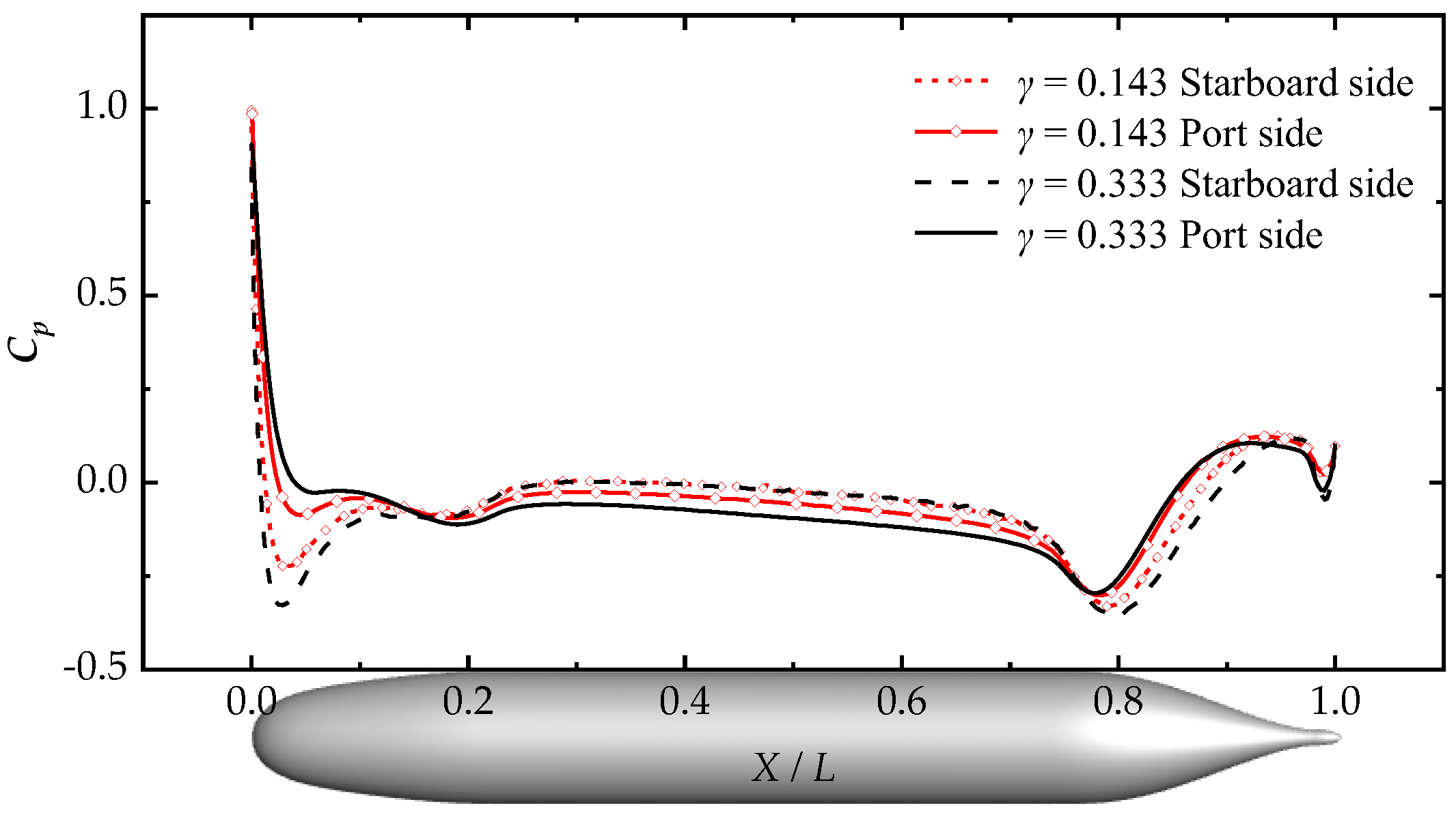
According to the results for the cases of straight navigation and steady turning motion at Fr = 0.5, the pressure coefficients of both sides are identical in the straight navigation case. The turning motion causes the pressure difference between the port side and starboard side. If the rotational radius changes and the same velocity of Fr = 0.5 of the submarine at the center of buoyancy is maintained, the difference in the pressure coefficient will significantly change when the submarine acquires the same orientation relative to the rotational center. The rotation rate, which relates to the ratio of the hull length to rotational radius, corresponds to = 0.333 (R = 3 L) and = 0.143 (R = 7 L), respectively. As shown in Figure 15, the dashed line and solid line marked with points represent the pressure coefficients of the starboard side and port side, respectively, at = 0.143. The gap in the pressure coefficient at X/L < 0.15 and X/L > 0.75, in the case of = 0.143, is much smaller than in the case of = 0.333. The effect of the rotation rate on the pressure coefficient is very minimal for the parallel middle body of the starboard when the submarine is forced in a turn to port. Nevertheless, the magnitude of the pressure coefficient on the port side becomes smaller as the rotation rate decreases. Hence, decreasing the rotation rate can reduce the pressure difference between the port and starboard sides.
The normal force, shown in Table 5, is greater than 0, meaning that the normal force is in the same direction as shown in Figure 13, when the submarine is forced in a turn to port. According to Table 5, the change in the tangential force is minimal when the submarine turns at the same velocity. However, the normal force decreases significantly as the rotational radius increases at the same time. The rotation rate γ, which represents the ratio of the length of the submarine to rotational radius, decreases accordingly as the rotational radius increases. The results of the tangential force indicate that rotation rate does not have much effect on the longitudinal pressure gradient, viscous shear stress gradient and wave-making intensity. In contrast, the normal component of the force is strongly influenced by the rotation rate of the submarine in the steady turning motion. The tangential force is much greater than normal force, so that the resultant force of the two force components shows a small decrease in this trend.
5. Conclusions
This study established a numerical model in FLUENT by using a combination of the dynamic layering mesh method and overset mesh technique in order to simulate the motion of the SUBOFF bare hull. The present approach solves the problem arising from a poor mesh quality, uncertainties in the exchange of data on the interface and the instability of the boundary conditions. It improves the mesh quality and avoids mesh deformation around the submarine, whereas before, the model needed to be re-meshed dynamically. In addition to the improvement of the accuracy of the simulation, the uncertainties of this approach are reduced compared with the sliding mesh method, which requires the exchanging of data on the interface. The total number of mesh cells in the model increases over the simulation time. It is possible to start with a small number of mesh cells to save computing costs. The model is proved to be feasible by comparing the numerical results with the experimental data in a straight navigation case. The conclusions of the present study are as follows:
- (1)
- The steady turning motion of the submarine causes the pressure difference between the port side and starboard side, which results from the difference in the velocity field distribution and the flow separation on both sides of the submarine. The velocity vector field on the plane of z = 0 reflects the characteristics of the flow field around the submarine during its turning motion. It can explain the surface pressure variation precisely through the analysis of the velocity vector field based on Bernoulli’s equation.
- (2)
- In the steady turning period, under the condition of the same rotation rate, the influences of the velocity on the wake waves, pressure coefficient and force are significant. The force components in both the tangential direction and normal direction increase as the velocity increases. This indicates that the forward velocity affects the flow field in terms of the pressure gradient, viscous shear stress gradient and wave-making intensity.
- (3)
- When the submarine retains the same velocity but changes in the rotation rate, the force component in the normal direction changes significantly. Decreasing the rotation rate will decrease the normal force. Thus, the normal force is strongly affected by the rotation rate. The tangential force tends to remain constant at the same time, indicating that it is independent of the rotation rate.
Even though the present approach improves numerical accuracy and efficiency, it has limitations as well. The cell height of each layer for the renewal of the mesh in the computational domain is fixed and cannot change during the calculation. Thus, it is necessary to choose a proper cell height ho in order to balance the numerical accuracy and efficiency. The C-type domain is suitable for obtaining the complete wake waves of the submarine under a turning motion. It is possible to shorten the computational domain when the simulations focus only on the hydrodynamic derivatives of the submarine.
Author Contributions
Study design by G.H.; data analysis by G.H.; literature search by C.Z., H.X. and S.L.; figures by C.Z. and H.X.; writing by C.Z.; validation by G.H. and H.X. All authors have read and agreed to the published version of the manuscript.
Funding
This work was funded by the Taishan Scholars Project of Shandong Province (tsqn201909172) and the University Young Innovational Team Program, Shandong Province (2019KJN003).
Institutional Review Board Statement
This study was approved by Institutional Review Board.
Informed Consent Statement
Informed Consent Statement was obtained from all subjects involved in the study.
Data Availability Statement
The data presented in this study are available on request from the corresponding author.
Conflicts of Interest
The authors declare no conflict of interest.
References
- Chen, Z.; Dai, Y.; Deng, F.; Ni, G. Mathematical model study and simulation analysis of submarine underwater rotary movement. Ship Sci. Technol. 2015, 37, 46–50. [Google Scholar]
- Zhang, L.; Deng, X.; Zhang, H. A review of dynamic mesh generation techniques and unsteady computing methods. Adv. Mech. 2010, 40, 424–447. [Google Scholar]
- Huang, C. Direct Simulation of Maneuver of the Underwater Vehicle Based on Overset Grid. Master’s Thesis, Wuhan University of Technology, Wuhan, China, 2018. [Google Scholar]
- Deng, F.; Dai, Y.; Chen, Z.; Zhang, B. Sliding mesh based on numerical simulation of rotating arms tests for submarines. Command. Control. Simul. 2016, 38, 122–126. [Google Scholar]
- Ma, Z.H.; Qian, L.; Martínez-Ferrer, P.J.; Causon, D.M.; Mingham, C.G.; Bai, W. An overset mesh based multiphase flow solver for water entry problems. Comput. Fluids 2018, 172, 689–705. [Google Scholar] [CrossRef] [Green Version]
- Sun, Z.; Liu, G.-J.; Zou, L.; Zheng, H.; Djidjeli, K. Investigation of Non-Linear Ship Hydroelasticity by CFD-FEM Coupling Method. J. Mar. Sci. Eng. 2021, 9, 511. [Google Scholar] [CrossRef]
- Windt, C.; Davidson, J.; Akram, B.; Ringwood, J.V. Performance Assessment of the Overset Grid Method for Numerical Wave Tank Experiments in the OpenFOAM Environment. In Proceedings of the ASME 2018 37th International Conference on Ocean, Offshore and Arctic Engineering, Madrid, Spain, 17–22 June 2018. [Google Scholar]
- Romano, A.; Lara, J.L.; Barajas, G.; Di Paolo, B.; Bellotti, G.; Di Risio, M.; Losada, I.J.; De Girolamo, P. Tsunamis Generated by Submerged Landslides: Numerical Analysis of the Near-Field Wave Characteristics. J. Geophys. Res. Ocean. 2020, 125, e2020JC016157. [Google Scholar] [CrossRef]
- Zaghi, S.; Mascio, A.D.; Broglia, R.; Muscari, R. Application of dynamic overlapping grids to the simulation of the flow around a fully-appended submarine. Math. Comput. Simul. 2015, 116, 75–88. [Google Scholar] [CrossRef]
- Cao, L.; Zhu, J.; Huang, K.; Ge, Y.; Wang, Z. Numerical simulation of a fully appended submarine model in steady turn. J. Nav. Univ. Eng. 2015, 27, 17–20. [Google Scholar]
- Zhang, D.; Yan, J.; Zhao, B.; Zhu, K. Numerical simulations of submarine rotating arms based on overset mesh. Sci. Technol. Eng. 2022, 22, 393–399. [Google Scholar]
- Mi, B.; Zhan, H.; Wang, B. Numerical simulation of dynamic derivatives based on rigid moving mesh technique. J. Aerosp. Power 2014, 29, 2659–2664. [Google Scholar] [CrossRef]
- Wu, J.; Zhang, E.; Zhong, L. Research on underwater vehicle’s thrust characteristics in the state of rotary motion. Ship Sci. Technol. 2018, 40, 1–7. [Google Scholar]
- Toxopeus, S.L.; Atsavapranee, P.; Wolf, E.; Daum, S.; Gerber, A.G. Collaborative CFD Exercise for a Submarine in a Steady Turn. In Proceedings of the International Conference on Ocean, Rio de Janeiro, Brazil, 1–6 July 2012. [Google Scholar]
- Lyu, X.; Tang, H.; Sun, J.; Wu, X.; Chen, X. Simulation of microbubble resistance reduction on a suboff model. Brodogr. Teor. I Praksa Brodogr. I Pomor. Teh. 2014, 65, 23–32. [Google Scholar]
- Cao, L.; Zhu, J.; Zeng, G. Viscous-Flow calculations of submarine maneuvering hydrodynamic coefficients and flow field based on same grid topology. J. Appl. Fluid Mech. 2016, 9, 817–826. [Google Scholar] [CrossRef]
- Pan, Y.; Zhou, Q.; Zhang, H. Numerical simulation of rotating arm test for prediction of submarine rotary derivatives. J. Hydrodyn. 2015, 27, 68–75. [Google Scholar] [CrossRef]
- Groves, N.C.; Huang, T.T.; Chang, M.S. Geometric Characteristics of DARPA (Defense Advanced Research Projects Agency) SUBOFF Models (DTRC Model Numbers 5470 and 5471); David Taylor Research Center Bethesda MD Ship Hydromechanics Department: Bethesda, MD, USA, 1989. [Google Scholar]
- Lin, J.; Ni, G.; Dai, Y.; Qu, D. Research on parameters’ change rule of submarine’s steady rotary movement. Ship Sci. Technol. 2014, 36, 31–33+37. [Google Scholar]
- Wang, X.; Lian, Z.; Xu, J.; Li, X. SUBOFF standard model underwater resistance test method. In Proceedings of the 14th National Congress on Hydrodynamics & the 28th National Conference on Hydrodynamics, Changchun, China, 8 August 2017; pp. 450–456. [Google Scholar]
- Liu, H.L.; Huang, T.T. Summary of DARPA Suboff Experimental Program Data; Defense Technical Information Center: Fort Belvoir, VA, USA, 1998. [Google Scholar]
- Liu, S.; He, G.; Wang, Z.; Luan, Z.; Zhang, Z.; Wang, W.; Gao, Y. Resistance and flow field of a submarine in a density stratified fluid. Ocean. Eng. 2020, 217, 107934. [Google Scholar] [CrossRef]
- Liu, S.; He, G.; Wang, W.; Gao, Y. Analysis on the wake of a shallow navigation submarine in the density-stratified fluid. J. Harbin Inst. Technol. 2021, 53, 52–59. [Google Scholar]
- Tang, Y. Study of Ship Turning Simulation Based on CFD. Master’s Thesis, Dalian Maritime University, Dalian, China, 2015. [Google Scholar]
- Liu, S.; He, G.; Wang, W.; Pan, Y. Effect of density stratification on wave-making resistance of submarine navigating in deep water. J. Harbin Eng. Univ. 2021, 42, 1373–1379. [Google Scholar]
Figure 1.
Schematic of the computational domain. (a) Straight navigation. (b) Steady turning motion.
Figure 1.
Schematic of the computational domain. (a) Straight navigation. (b) Steady turning motion.
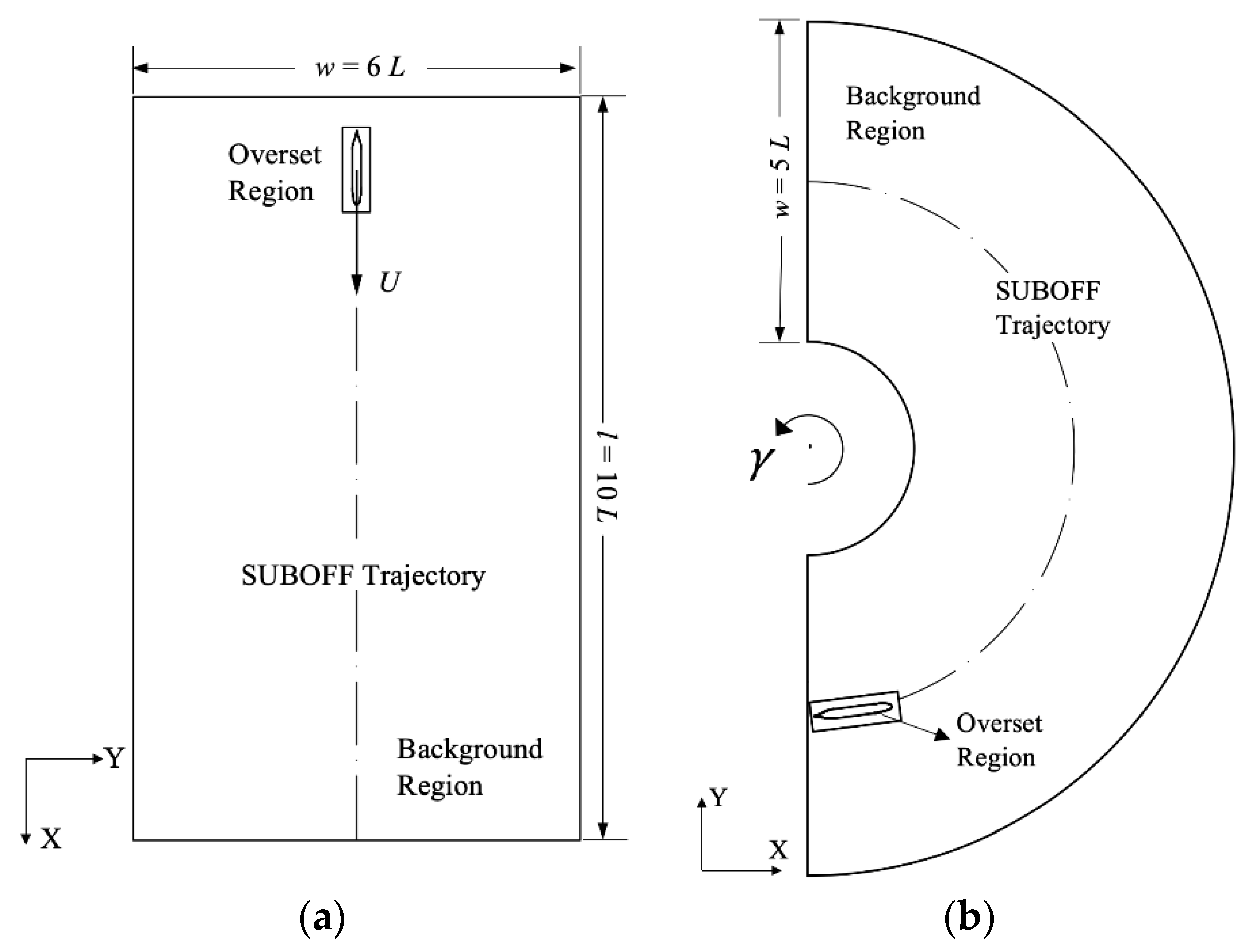
Figure 2.
Initial grids of the computational domain. (a) Straight navigation. (b) Steady turning motion, (c) Overset region section profile.
Figure 2.
Initial grids of the computational domain. (a) Straight navigation. (b) Steady turning motion, (c) Overset region section profile.
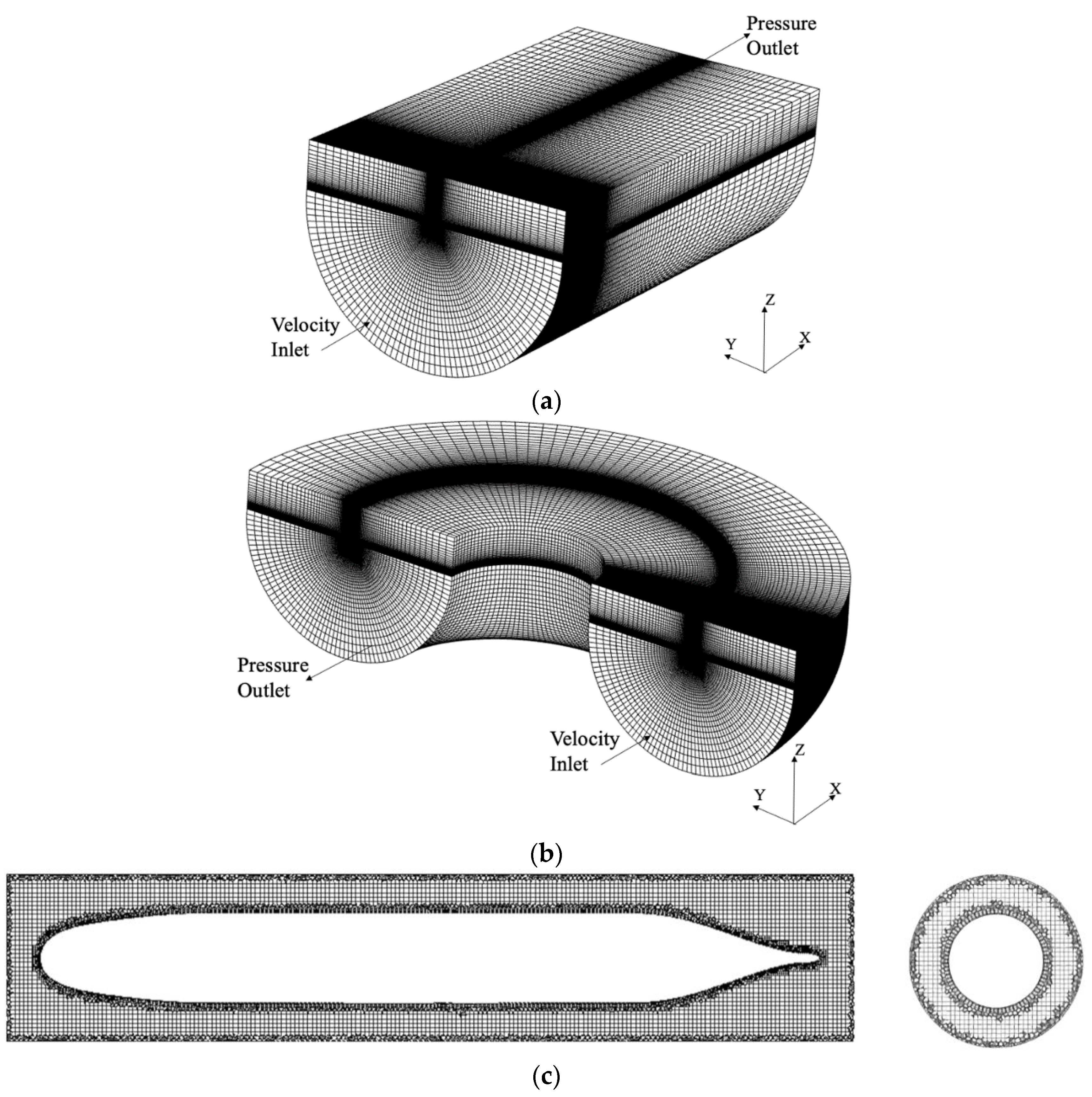
Figure 3.
Mesh topologies (top view). (a) Initial mesh, (b) Renewal of mesh, (c) Initial mesh, (d) Renewal of mesh.
Figure 3.
Mesh topologies (top view). (a) Initial mesh, (b) Renewal of mesh, (c) Initial mesh, (d) Renewal of mesh.

Figure 4.
Validation of the resistance results.

Figure 5.
Validation of the pressure coefficient along the upper meridian.

Figure 6.
Velocity vector field at z = 0 with the two methods.
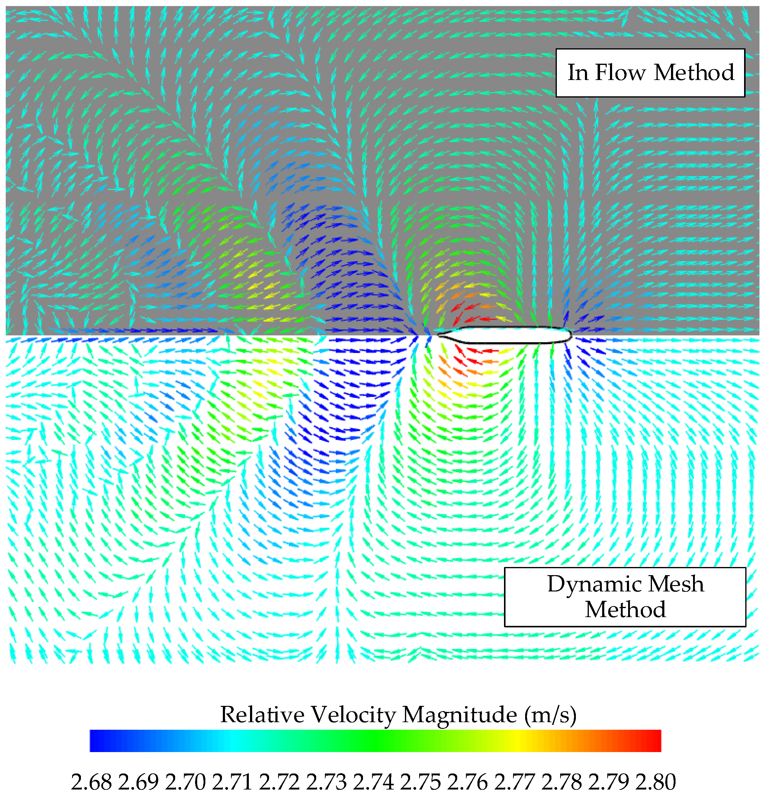
Figure 7.
Wave profile on the free surface.
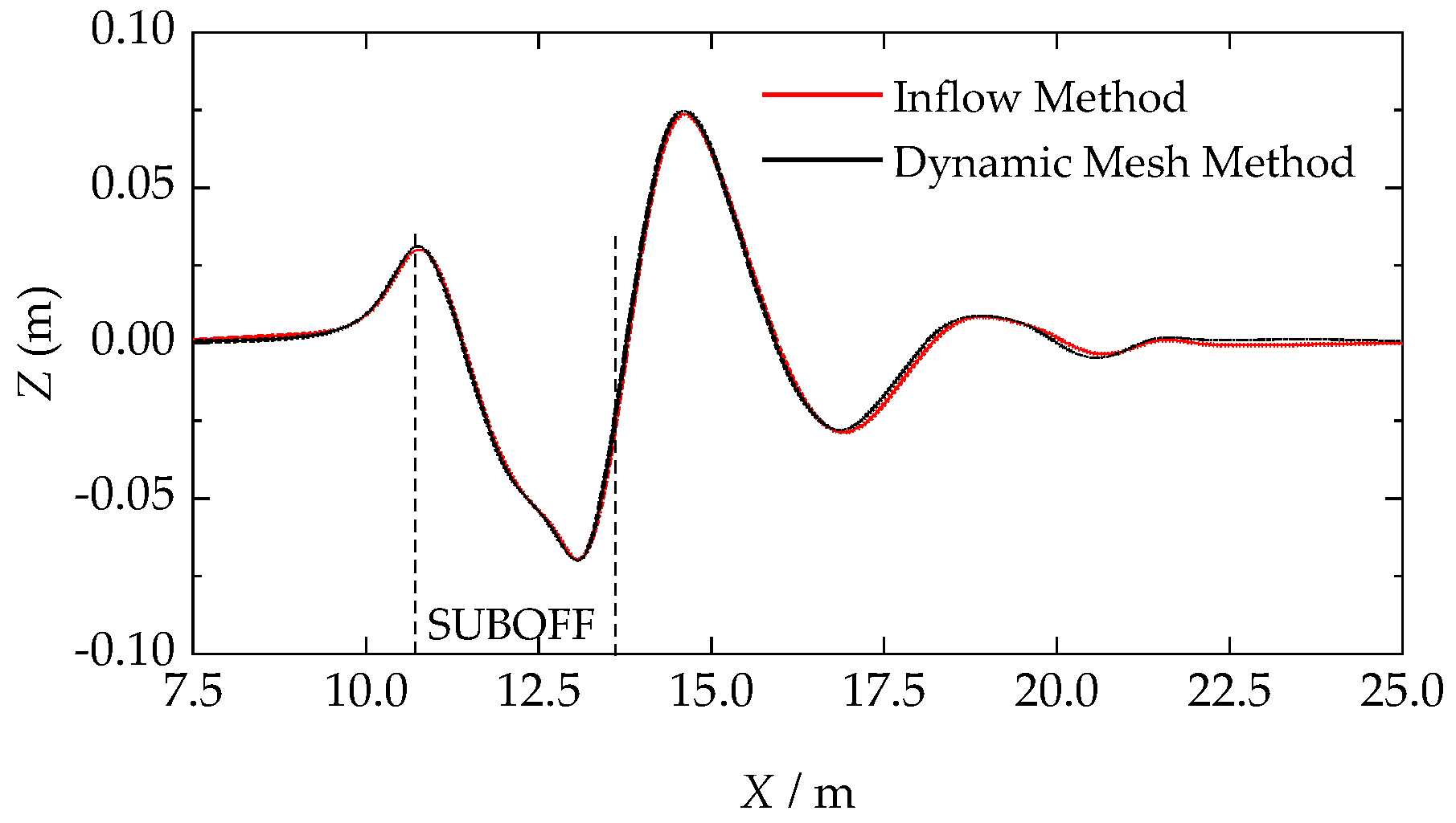
Figure 8.
Development of wakes at the free surface at Fr = 0.5. (a) t = 5 s, (b) t = 10 s, (c) t = 15 s.
Figure 8.
Development of wakes at the free surface at Fr = 0.5. (a) t = 5 s, (b) t = 10 s, (c) t = 15 s.
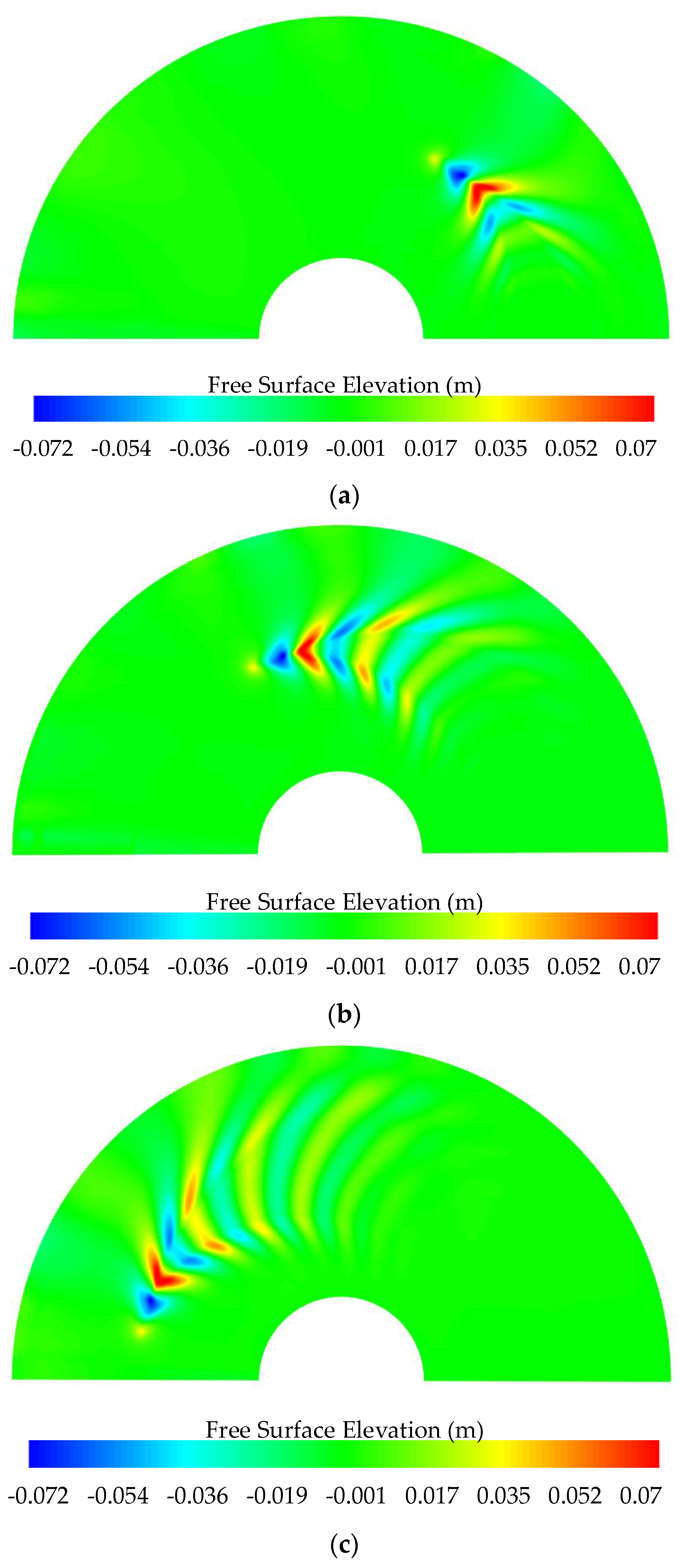
Figure 9.
Characteristics of wakes at the free surface at different velocities. (a) Fr = 0.3, (b) Fr = 0.5, (c) Fr = 0.7.
Figure 9.
Characteristics of wakes at the free surface at different velocities. (a) Fr = 0.3, (b) Fr = 0.5, (c) Fr = 0.7.

Figure 10.
Pressure coefficients along the meridians of the port side and starboard side for different motion types.
Figure 10.
Pressure coefficients along the meridians of the port side and starboard side for different motion types.
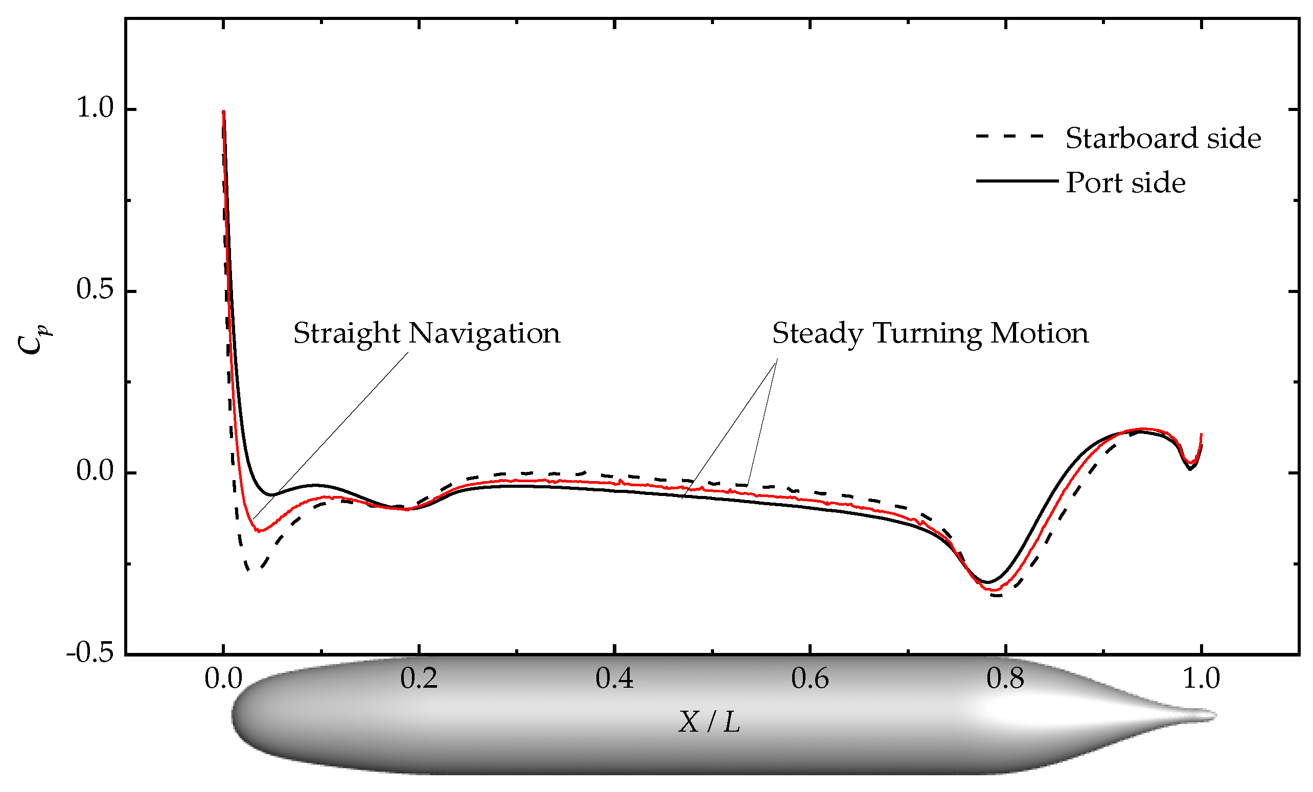
Figure 11.
Velocity vector field on the plane of z = 0.
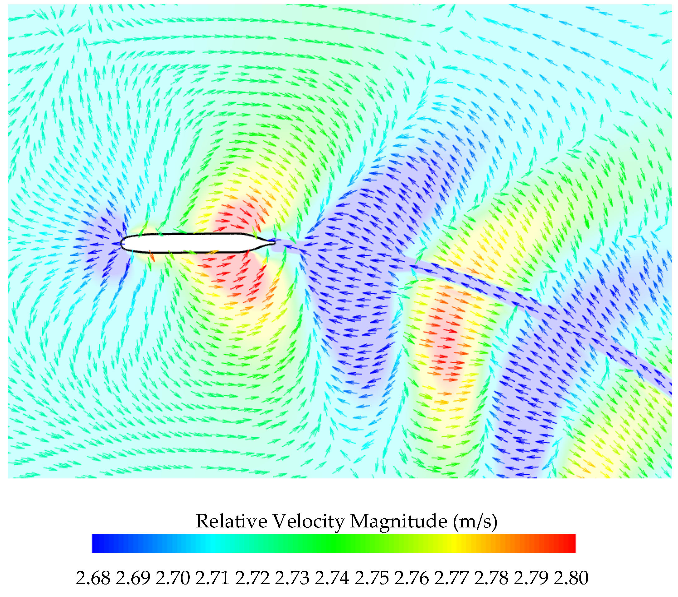
Figure 12.
Pressure coefficients along the meridians of the port side and starboard side at different velocities. (a) Starboard side. (b) Port side.
Figure 12.
Pressure coefficients along the meridians of the port side and starboard side at different velocities. (a) Starboard side. (b) Port side.
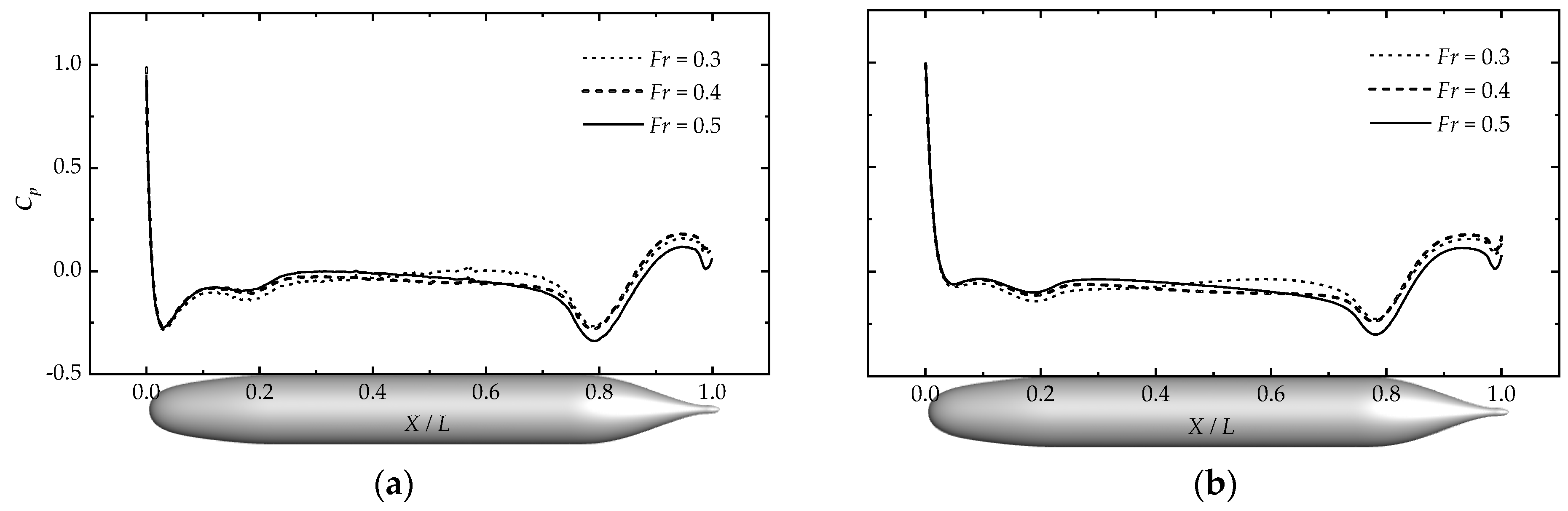
Figure 13.
Schematic of the force components.
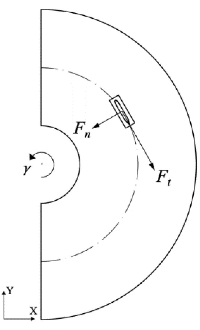
Figure 14.
Force component at varying velocities at the center of buoyancy. (a) The tangential component of resistance. (b) The normal component of resistance.
Figure 14.
Force component at varying velocities at the center of buoyancy. (a) The tangential component of resistance. (b) The normal component of resistance.
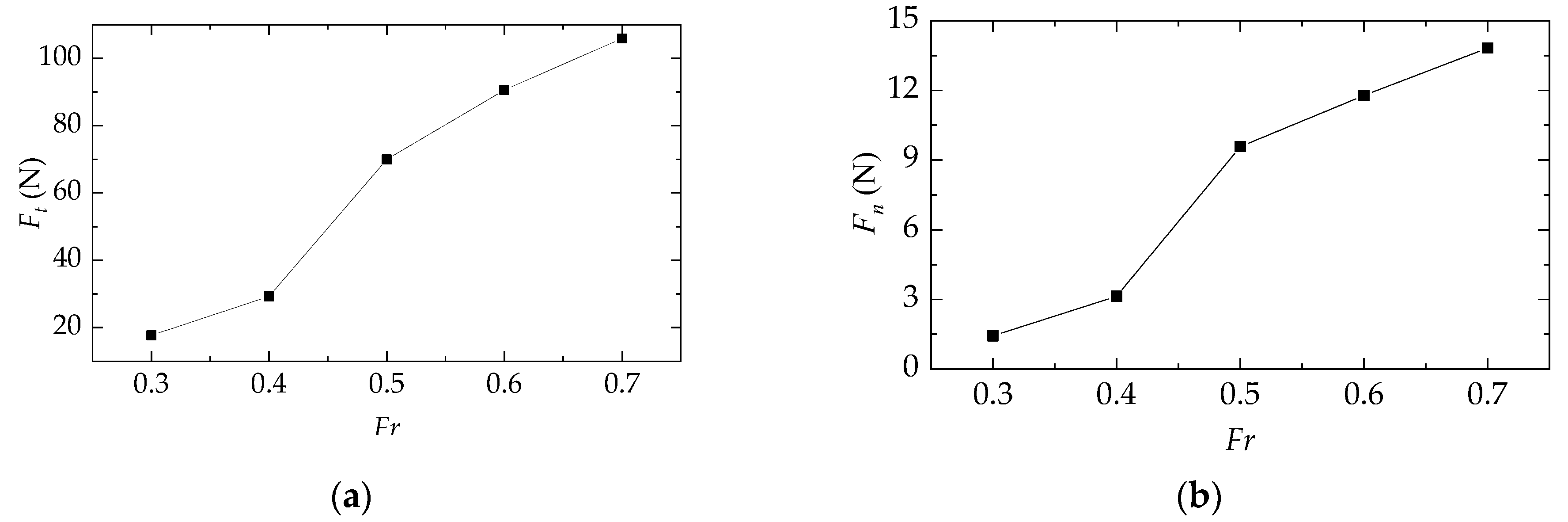
Figure 15.
Pressure coefficients along the meridians of the port side and starboard side at different rotation rates.
Figure 15.
Pressure coefficients along the meridians of the port side and starboard side at different rotation rates.

Table 1.
Mesh convergence analysis for straight navigation.
| Basic Size(m) | Net Increase in Cells (Thousand/s) | Total Resistance Rt (N) | Error of Rt (%) |
|---|---|---|---|
| 0.042 | 412.528 | 70.465 | —— |
| 0.063 | 324.429 | 70.461 | 0.006 |
| 0.084 | 206.963 | 69.984 | 0.683 |
| 0.126 | 128.653 | 69.404 | 1.507 |
Table 2.
Time step convergence analysis for straight navigation.
| Time Step (s) | Number of Steps (Step) | Total Resistance Rt (N) | Error of Rt (%) |
|---|---|---|---|
| 0.005 | 1000 | 70.829 | —— |
| 0.01 | 500 | 70.461 | 0.520 |
| 0.02 | 250 | 69.291 | 2.172 |
| 0.05 | 100 | 68.568 | 3.193 |
Table 3.
Mesh convergence analysis for steady turning.
| Basic Size(m) | Net Increase in Cells (Thousand/s) | Total Resistance Rt (N) | Error of Rt (%) |
|---|---|---|---|
| 0.0315 | 225.763 | 71.749 | —— |
| 0.042 | 170.822 | 71.342 | 0.568 |
| 0.063 | 115.586 | 70.653 | 1.529 |
| 0.084 | 83.421 | 69.976 | 2.471 |
Table 4.
Time step convergence analysis for steady turning.
| Time Step (s) | Number of Steps (Step) | Total Resistance Rt (N) | Error of Rt (%) |
|---|---|---|---|
| 0.005 | 1000 | 71.816 | —— |
| 0.01 | 500 | 71.342 | 0.660 |
| 0.02 | 250 | 70.388 | 1.989 |
| 0.05 | 100 | 69.720 | 2.918 |
Table 5.
Force component of the submarine at different rotation rates at Fr = 0.5.
| Froude Number Fr (-) | Rotational Radius R (m) | Rotation Rate γ = L/R (-) | Tangential Force Ft (N) | Normal Force Fn (N) | Resultant Force Rt (N) |
|---|---|---|---|---|---|
| 0.5 | 3 L | 0.333 | 69.305 | 19.665 | 72.041 |
| 5 L | 0.200 | 69.938 | 9.575 | 70.590 | |
| 7 L | 0.143 | 69.970 | 3.441 | 70.216 |
Publisher’s Note: MDPI stays neutral with regard to jurisdictional claims in published maps and institutional affiliations. |
© 2022 by the authors. Licensee MDPI, Basel, Switzerland. This article is an open access article distributed under the terms and conditions of the Creative Commons Attribution (CC BY) license (https://creativecommons.org/licenses/by/4.0/).
Share and Cite
MDPI and ACS Style
He, G.; Zhang, C.; Xie, H.; Liu, S. The Numerical Simulation of a Submarine Based on a Dynamic Mesh Method. J. Mar. Sci. Eng. 2022, 10, 1417. https://doi.org/10.3390/jmse10101417
AMA Style
He G, Zhang C, Xie H, Liu S. The Numerical Simulation of a Submarine Based on a Dynamic Mesh Method. Journal of Marine Science and Engineering. 2022; 10(10):1417. https://doi.org/10.3390/jmse10101417
Chicago/Turabian StyleHe, Guanghua, Cheng Zhang, Hongfei Xie, and Shuang Liu. 2022. "The Numerical Simulation of a Submarine Based on a Dynamic Mesh Method" Journal of Marine Science and Engineering 10, no. 10: 1417. https://doi.org/10.3390/jmse10101417
Note that from the first issue of 2016, this journal uses article numbers instead of page numbers. See further details here.