
An Optimal BP Neural Network Track Prediction Method Based on a GA–ACO Hybrid Algorithm


Abstract
:1. Introduction
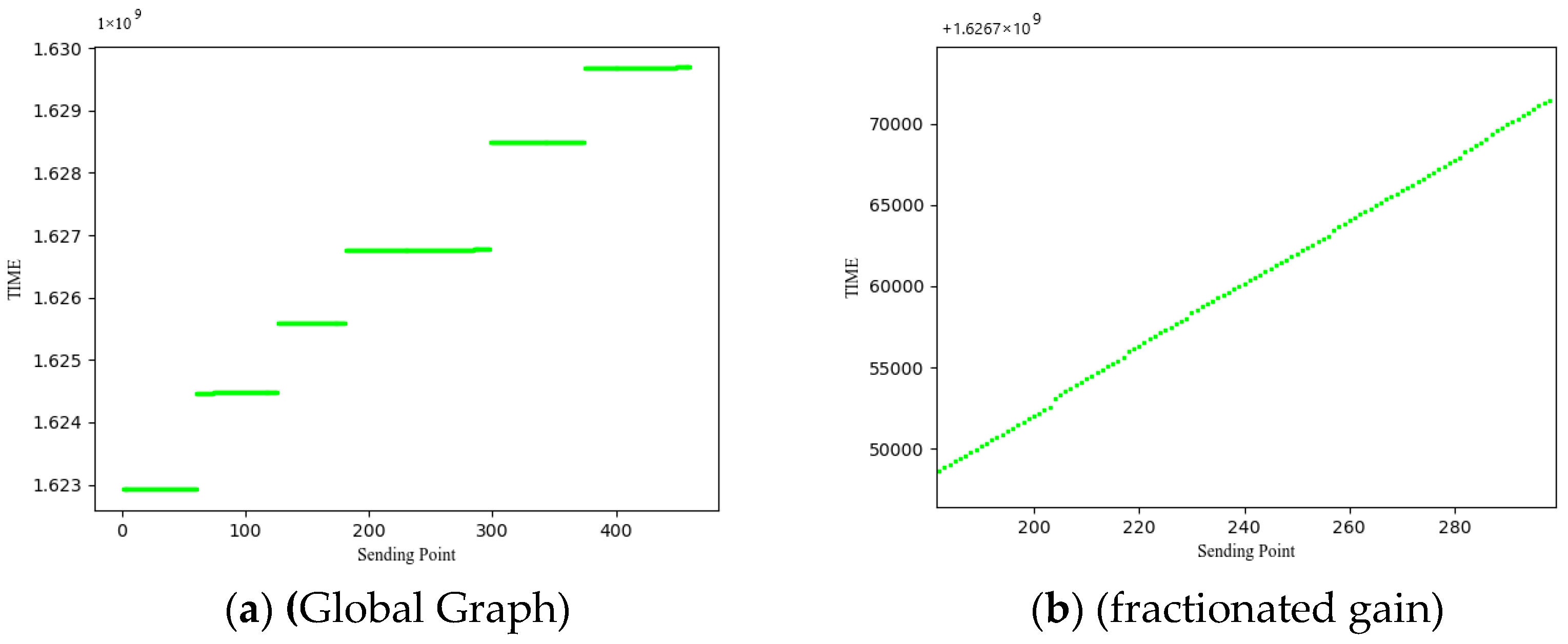
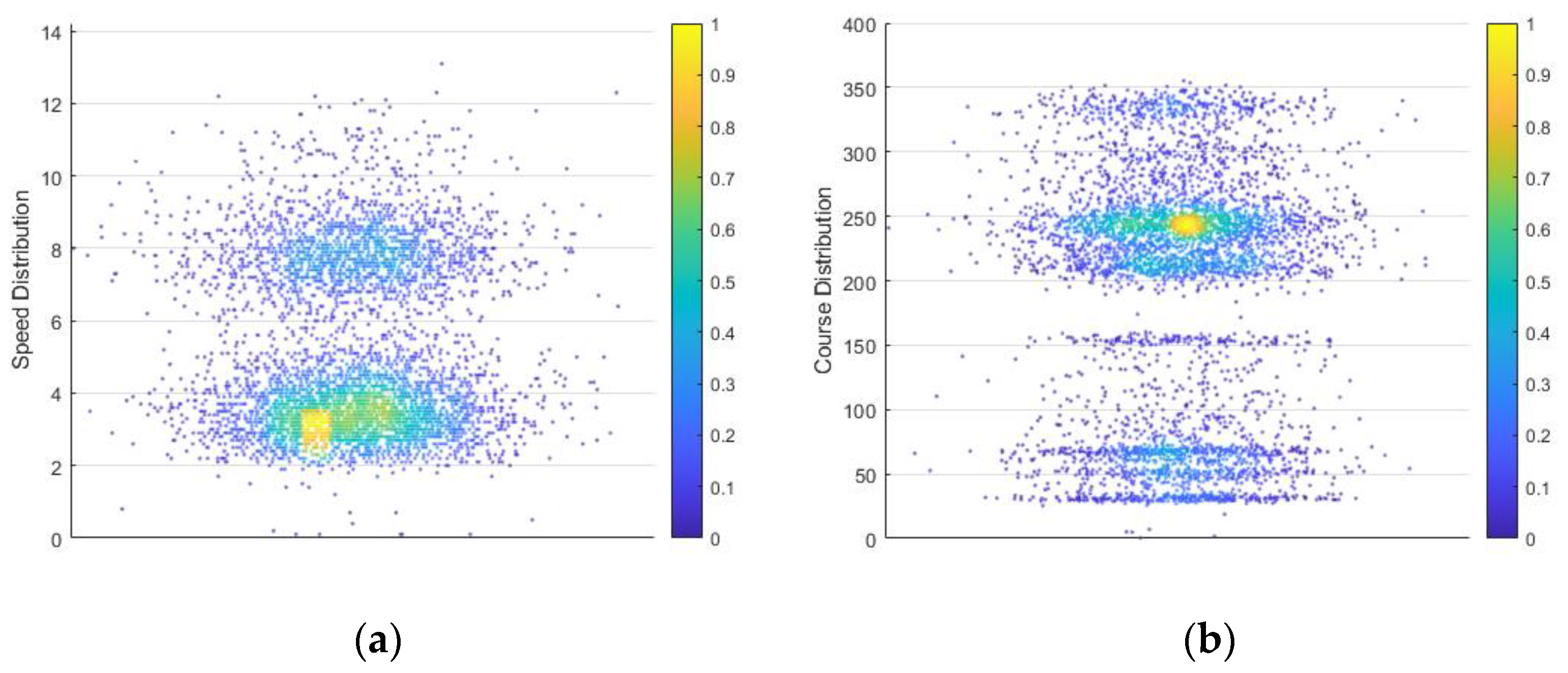
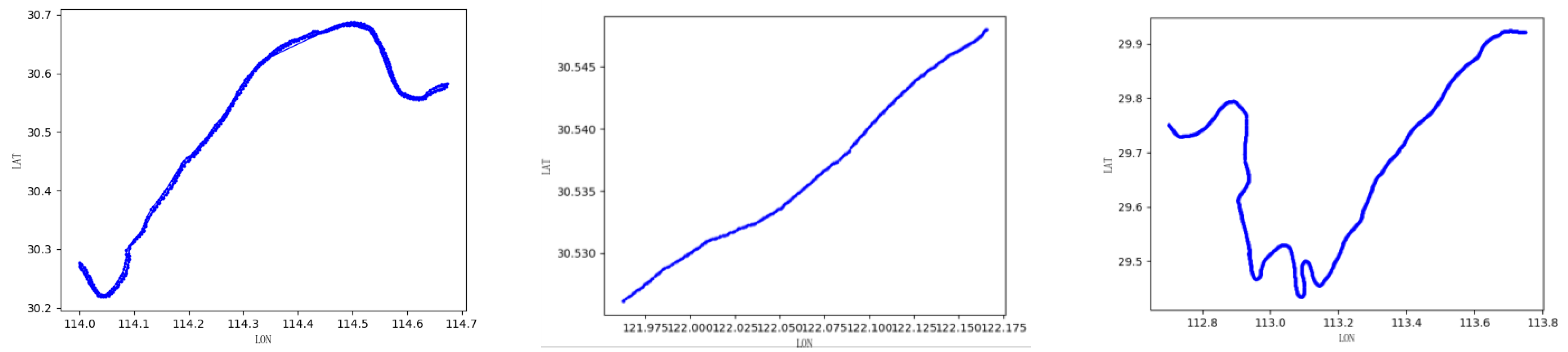
2. Data Preprocessing
| Algorithms 1. AIS data preprocessing |
| Data preprocessing pseudocode |
| 1: Connect to the database. |
| 2: Get Ni; where i in Len(N);//N is the total number of Trajectories. // |
| 3: if Ni.mmsi = Ni−1.mmsi &&R; Ni.sog ∈ [1 kn, 15 kn] && Ni.Δt: <300 s |
| //sog is the speed of the vessel, Δt is the time interval between two-state. // |
| 4: then Optimization (Ui), ;//Optimize (-) is the trajectory optimizing function. // |
| Return: Ui |
3. Design of a Track Prediction Model Integrating Multi-Technology
3.1. Design Idea
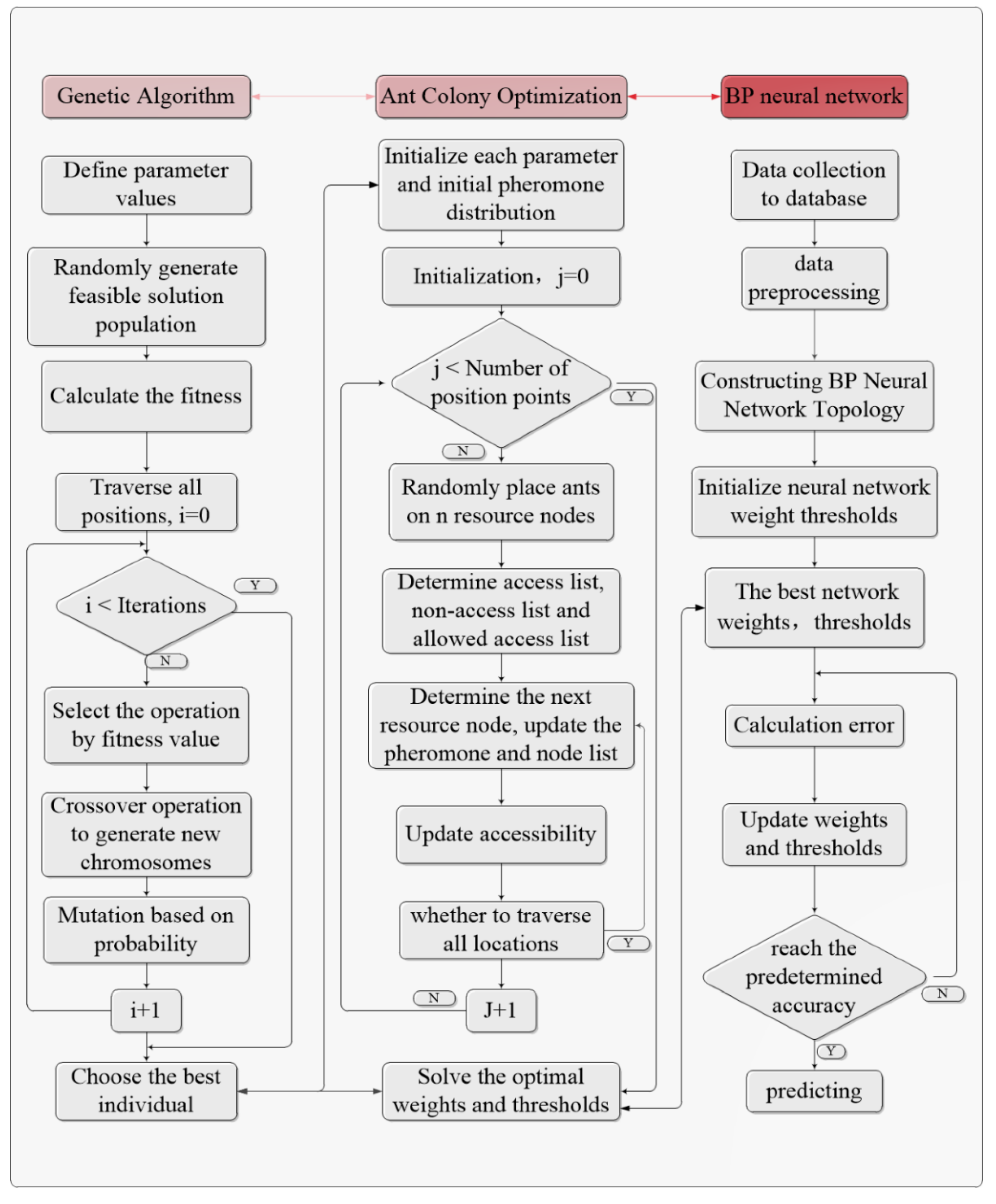
3.2. The GA–ACO–BP Hybrid Algorithm
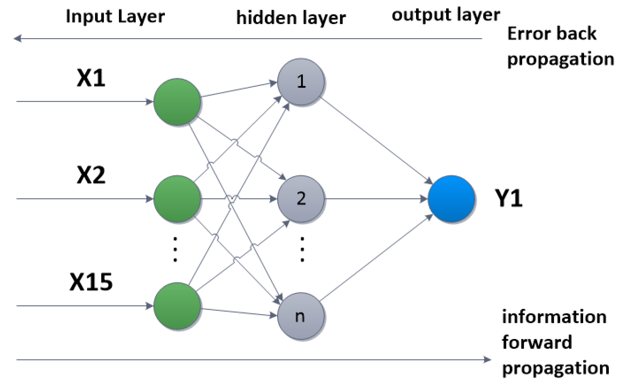
3.2.1. The BP Neural Network
3.2.2. Ant Colony Optimization
3.2.3. The Genetic Algorithm
3.3. The Track Prediction Model
4. Experimental Results and Analysis
4.1. Performance Indicators
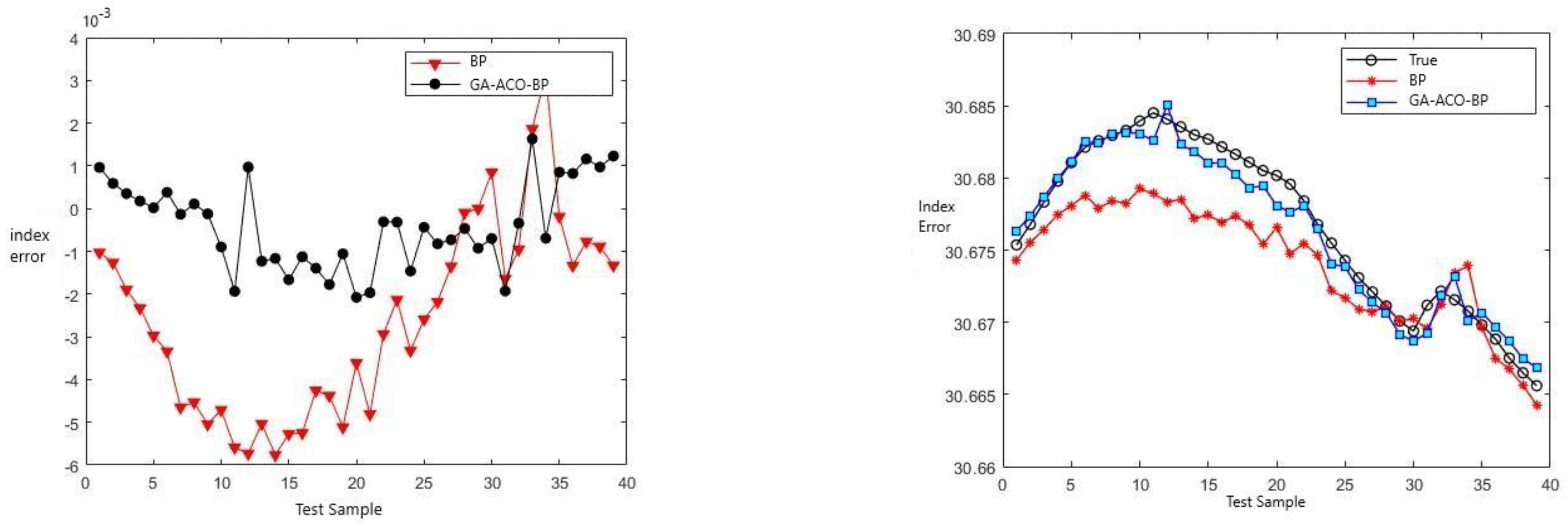
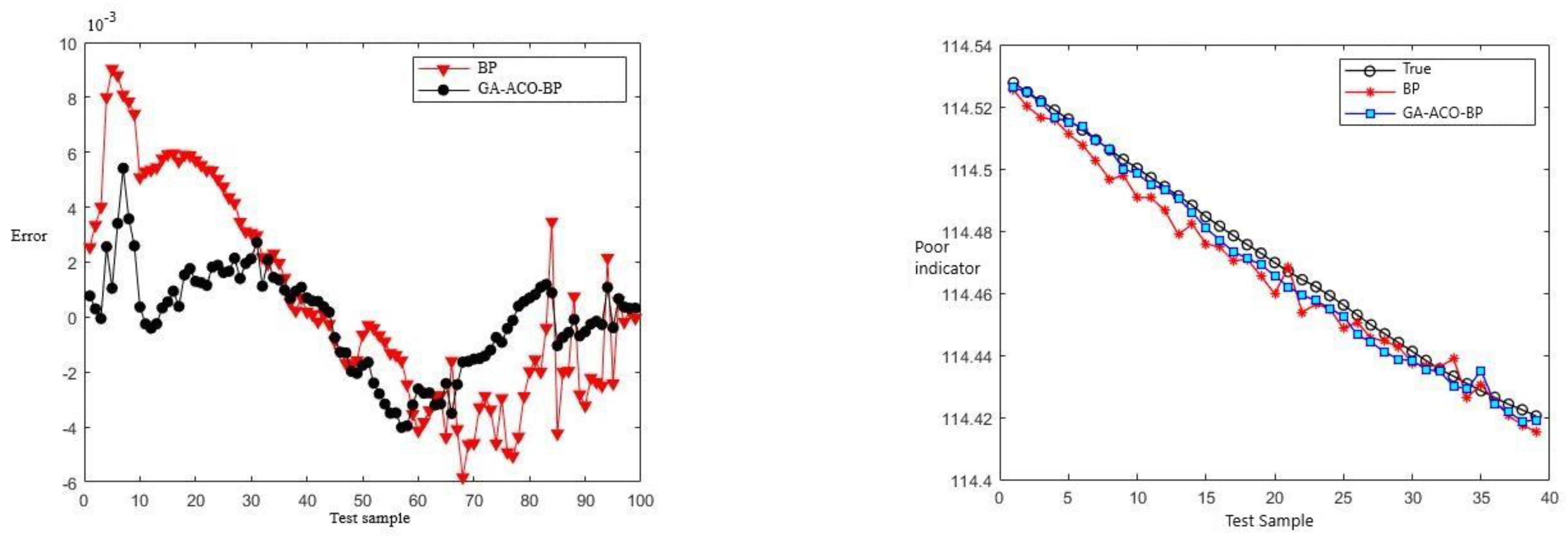
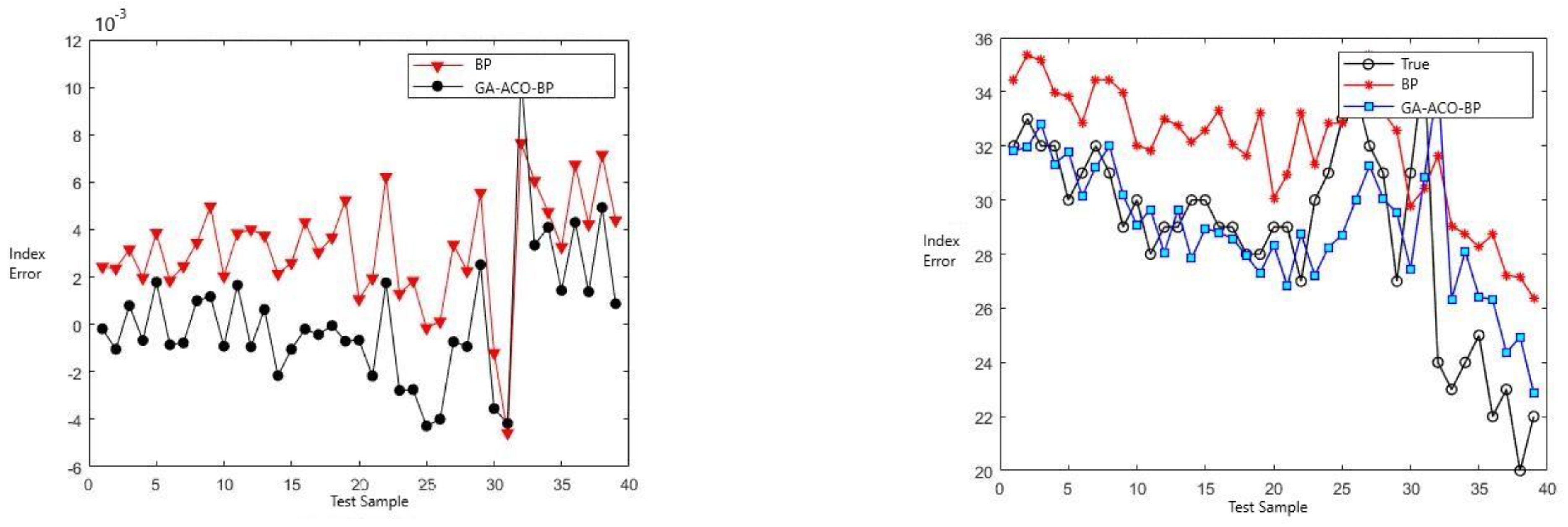
4.2. Analysis of Results
5. Conclusions
Author Contributions
Funding
Institutional Review Board Statement
Informed Consent Statement
Data Availability Statement
Conflicts of Interest
References
- Yoo, Y.; Kim, T. An Improved Ship Collision Risk Evaluation Method for Korea Maritime Safety Audit Considering Traffic Flow Characteristics. J. Mar. Sci. Eng. 2019, 7, 448. [Google Scholar] [CrossRef]
- He, Z.; Shao, Z.; Zeng, J. Ship navigation safety risk assessment based on genetic algorithm and BP neural network. Sci. Res. Rev. 2020, 13, 117. [Google Scholar]
- Xu, T.; Zhang, Q. Ship Traffic Flow Prediction in Wind Farms Water Area Based on Spatiotemporal Dependence. J. Mar. Sci. Eng. 2022, 10, 295. [Google Scholar] [CrossRef]
- Lv, P.; Zhuang, Y.; Yang, K. Prediction of Ship Traffic Flow Based on BP Neural Network and Markov Model. MATEC Web Conf. 2016, 81, 04007. [Google Scholar] [CrossRef]
- Bukhari, A.C.; Tusseyeva, I.; Kim, Y.G. An intelligent real-time multi-vessel collision risk assessment system from VTS view point based on fuzzy inference system. Expert Syst. Appl. 2013, 40, 1220–1230. [Google Scholar] [CrossRef]
- Xiao, F.; Ligteringen, H.; van Gulijk, C.; Ale, B. Comparison study on AIS data of ship traffic behavior. Ocean. Eng. 2015, 95, 84–93. [Google Scholar] [CrossRef]
- Brian, M.; Prasad, P.L. Ship behavior prediction via trajectory extraction-based clustering for maritime situation awareness. J. Ocean. Eng. Sci. 2021, 7, 1–13. [Google Scholar]
- Capobianco, S.; Millefiori, L.M.; Forti, N.; Braca, P.; Willett, P. Deep Learning Methods for Vessel Trajectory Prediction based on Recurrent Neural Networks. IEEE Trans. Aerosp. Electron. Syst. 2021, 57, 4329–4346. [Google Scholar] [CrossRef]
- Suo, Y.; Chen, W.; Claramunt, C.; Yang, S. A Ship Trajectory Prediction Framework Based on a Recurrent Neural Network. Sensors 2020, 20, 5133. [Google Scholar] [CrossRef] [PubMed]
- Qian, L.; Zheng, Y.; Li, L.; Ma, Y.; Zhou, C.; Zhang, D. A New Method of Inland Water Ship Trajectory Prediction Based on Long Short-Term Memory Network Optimized by Genetic Algorithm. Appl. Sci. 2022, 12, 4073. [Google Scholar] [CrossRef]
- Liu, Y.; Duan, W.; Huang, L.; Duan, S.; Ma, X. The input vector space optimization for LSTM deep learning model in real-time prediction of ship motions. Ocean. Eng. 2020, 213, 107681. [Google Scholar] [CrossRef]
- Tang, H.; Yin, Y.; Shen, H. A model for vessel trajectory prediction based on long short-term memory neural network. J. Mar. Eng. Technol. 2022, 21, 136–145. [Google Scholar] [CrossRef]
- Zhi-Jun, W.; Shan Tian, L.M. A 4D Trajectory Prediction Model Based on the BP Neural Network. J. Intell. Syst. 2019, 29, 1545–1557. [Google Scholar]
- Song, L.; Shengli, W.; Dingbao, X. Radar track prediction method based on BP neural network. J. Eng. 2019, 2019, 8051–8055. [Google Scholar] [CrossRef]
- Zhou, H.; Chen, Y.; Zhang, S. Ship Trajectory Prediction Based on BP Neural Network. J. Artif. Intell. 2019, 1, 29–36. [Google Scholar] [CrossRef]
- Rong, H.; Teixeira, A.P.; Soares, C.G. Ship trajectory uncertainty prediction based on a Gaussian Process model. Ocean Eng. 2019, 182, 499–511. [Google Scholar] [CrossRef]
- Wen-ying, J.; Yan, L.; Ming, C. An ant colony optimization–genetic algorithm approach for ship pipe route design. Int. Shipbuild. Prog. 2014, 61, 163–183. [Google Scholar]
- Dong, H.C.; Dong, Z.M. Surrogate-assisted grey wolf optimization for high-dimensional, computationally ex pensive black-box problems. Swarm Evol. Ary Comput. 2020, 57, 100713. [Google Scholar] [CrossRef]
- Deng, H.B.; Peng, L.Z.; Zhang, H.B.; Yang, B.; Chen, Z. Ranking based biased learning swarm optimizer for large-scale optimization. Inf. Sci. 2019, 493, 120–137. [Google Scholar] [CrossRef]


| DATA SET | AIS |
|---|---|
| Position | Wuhan |
| Period | 21 June 2021–21 July 2021 19 May 2022–20 May 2022 |
| Time interval | <3 min |
| Raw data | 10,497,031 |
| Total number of tracks after processing | 571 |
| Total AIS data after processing | 180,647 |
| Input indicator | TIME/LON/LAT/SOG/COG/A/ROT |
| Output indicator | LON/LAT/TIME/SOG |
| Name | Value |
|---|---|
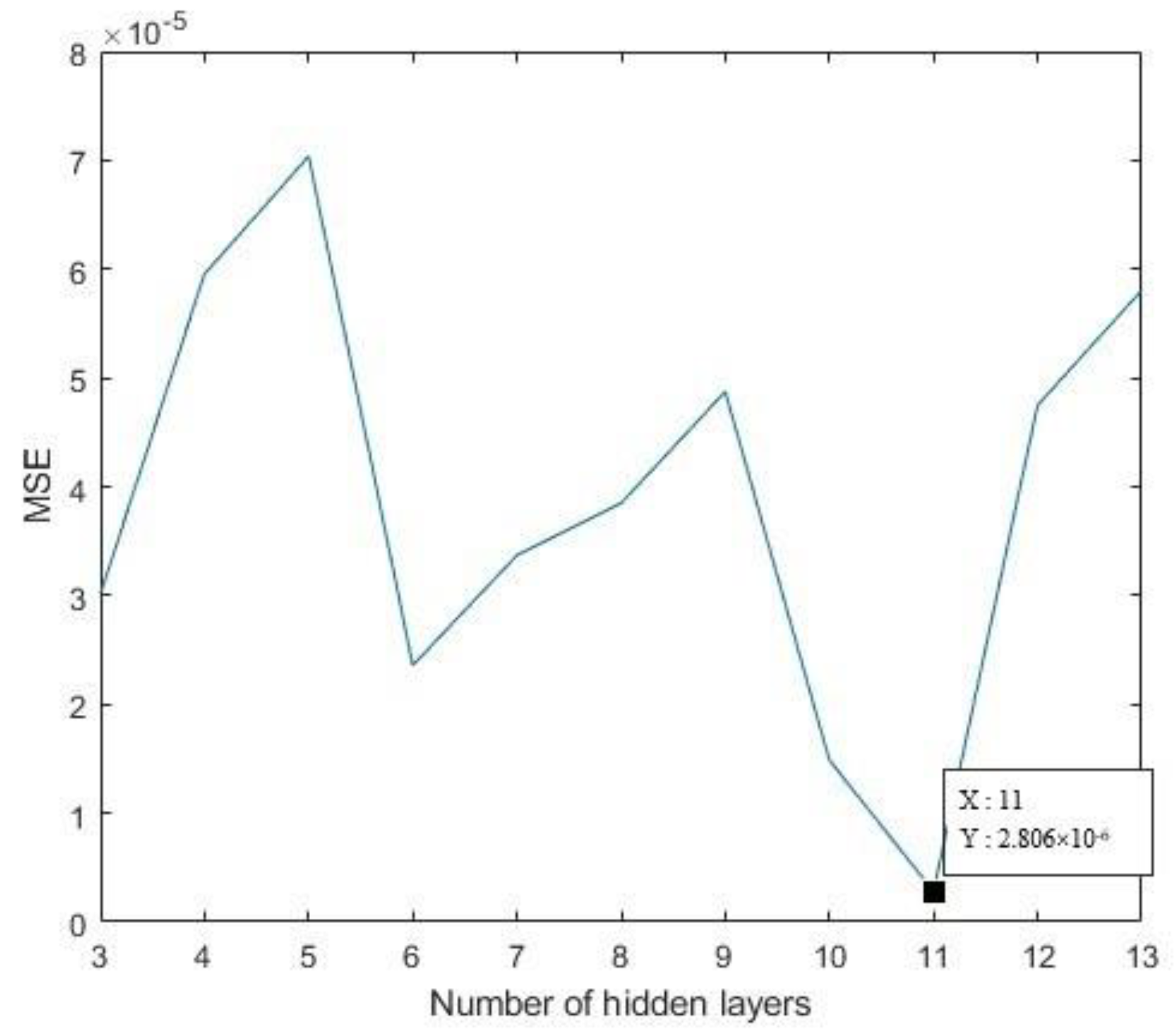
| Hidden layer nodes | 11 |
| Learn rate | 0.001 |
| Target error | 0.0001 |
| Time step | 25 |
| epochs | 100 |
| Min_grad | 10−6 |
| Name | Value | |
|---|---|---|
| GA | Population size | 30 |
| Hybrid rate | 0.6 | |
| Mutation rate | 0.2 | |
| MaxGeneration | 50 | |
| ACO | MaxGeneration | 100 |
| Ant size | 30 | |
| Time step | 25 | |
| volatility coefficient | 0.3 | |
| Min_grad | 10−6 |
| Network Model | MAE | MSE | RMSE | MAPE |
|---|---|---|---|---|
| LSTM | 0.0030329 | 4.8574 × 10⁻⁶ | 0.0022114 | 0.005752% |
| BP neural network | 0.0031725 | 7.4802 × 10⁻⁴ | 0.0038473 | 0.01036% |
| GA–BP neural network | 0.0020121 | 8.2417 × 10⁻⁵ | 0.0022972 | 0.006271% |
| ACO–BP neural network | 0.0040795 | 2.3528 × 10⁻⁵ | 0.0048506 | 0.0035635% |
| GA–ACO–BP neural network | 0.0014547 | 3.3217 × 10⁻⁶ | 0.0018226 | 0.0027472% |
| Neural Network | Training Duration (s) | Test Duration (s) | ||
|---|---|---|---|---|
| prediction accuracy | 10−4 | 10−5 | 10−4 | 10−5 |
| GA–BP | 45.785745 | 50.524558 | 0.0025646 | 0.0034546 |
| GA–ACO–BP | 32.714566 | 35.456464 | 0.038456 | 0.0039457 |
| ACO–BP | 60.564647 | 67.454645 | 0.0067544 | 0.0078651 |
| LSTM | 41.845995 | 47.456664 | 0.0039671 | 0.0045783 |
| Neural Network | Training Duration (s) | Test Duration (s) | ||
|---|---|---|---|---|
| prediction accuracy | 10−4 | 10−5 | 10−4 | 10−5 |
| GA–BP | 42.546455 | 45.832545 | 0.0018112 | 0.0022972 |
| GA–ACO–BP | 37.546544 | 41.546544 | 0.0036457 | 0.0038473 |
| ACO–BP | 50.457531 | 55.45788 | 0.0058371 | 0.0063040 |
| LSTM | 31.874541 | 37.418444 | 0.0038757 | 0.0039603 |
Publisher’s Note: MDPI stays neutral with regard to jurisdictional claims in published maps and institutional affiliations. |
© 2022 by the authors. Licensee MDPI, Basel, Switzerland. This article is an open access article distributed under the terms and conditions of the Creative Commons Attribution (CC BY) license (https://creativecommons.org/licenses/by/4.0/).
Share and Cite
Zheng, Y.; Lv, X.; Qian, L.; Liu, X. An Optimal BP Neural Network Track Prediction Method Based on a GA–ACO Hybrid Algorithm. J. Mar. Sci. Eng. 2022, 10, 1399. https://doi.org/10.3390/jmse10101399
Zheng Y, Lv X, Qian L, Liu X. An Optimal BP Neural Network Track Prediction Method Based on a GA–ACO Hybrid Algorithm. Journal of Marine Science and Engineering. 2022; 10(10):1399. https://doi.org/10.3390/jmse10101399
Chicago/Turabian StyleZheng, Yuanzhou, Xuemeng Lv, Long Qian, and Xinyu Liu. 2022. "An Optimal BP Neural Network Track Prediction Method Based on a GA–ACO Hybrid Algorithm" Journal of Marine Science and Engineering 10, no. 10: 1399. https://doi.org/10.3390/jmse10101399
APA StyleZheng, Y., Lv, X., Qian, L., & Liu, X. (2022). An Optimal BP Neural Network Track Prediction Method Based on a GA–ACO Hybrid Algorithm. Journal of Marine Science and Engineering, 10(10), 1399. https://doi.org/10.3390/jmse10101399