Study of the LQRY-SMC Control Method for the Longitudinal Motion of Fully Submerged Hydrofoil Crafts

Abstract

The control system is one of the important components of the hydrofoil craft. By adjusting the navigation attitude of the craft, the hydrofoil craft can navigate stably and safely in the turbulent environment. Aiming at the problem that existing control algorithms have poor stability in the longitudinal motion control of hydrofoil craft, the longitudinal motion reduction is limited, and there are excessive requirements for accurate disturbance wave data. Based on the fully submerged hydrofoil craft model, this article proposes a joint control method LQRY-SMC combining linear-quadratic optimal control with output regulation (LQRY) and sliding-mode control (SMC), and adds genetic algorithm to optimize the weighting matrix parameters, get better control-feedback gain, improve the global optimal-control stability, thus improving the comfort of the crew, and prevent the attack of the hull, deck wetness and damage to instruments. The simulation results show that compared with the existing methods, the heave displacement and pitch angle obtained by LQRY-SMC under the turbulent flow of different significant wave heights are reduced by about 50%, and the influence of longitudinal motion on hydrofoil crafts is avoided to a large extent, which proves the effectiveness and superiority of the method proposed.

1. Introduction

The fully submerged hydrofoil craft is a new type of high-performance ship. When sailing at high speed, the hydrofoil installed at the bottom of the craft body is used to generate hydrodynamic lift to lift part or all of the craft body off the water surface, so as to reduce the resistance and improve the sailing speed. The maximum speed can reach more than 50 knots. Compared with traditional ships, it has the characteristics of low resistance, high speed and good seakeeping. The appearance of hydrofoil crafts enables people to save time at sea and obtain a more comfortable shipping experience. However, under the interference of sea waves, hydrofoil crafts will inevitably produce heave and pitch motion, which seriously affects the comfort and work efficiency of the crew. On the other hand, the intense longitudinal movement will cause damage to the onboard instruments and equipment, increase the probability of the attack of the hull, deck wetness, and even hydrofoil out of the water, bring danger to navigation [1].

In order to make the hydrofoil craft navigate stably and safely in the turbulent environment, an important way is to add a control algorithm to the longitudinal motion system of the hydrofoil craft to reduce the heave displacement and pitch angle to a certain extent. By controlling the control surface of the hydrofoil trailing edge flap of the hydrofoil craft, the lift of the hydrofoil craft can be continuously adjusted to offset the interference of the waves and improve the seakeeping performance of the hydrofoil craft. At present, the most commonly used control methods of hydrofoil crafts are based on the improved PID algorithm or classical robust control, and for this multi-input and multi-output nonlinear strong coupling system with uncertain disturbance and unknown parameter disturbance, the above method has poor application effect, large error and cannot meet the requirements. Therefore, many scholars convert the nonlinear model into a linear model for research [2,3,4]. The longitudinal motion control system of ships can be traced back to the 1950s. Matdaud Z. summarized the key technologies used by the United States and the Soviet Union to control the longitudinal motion of ground-effect ships to stabilize ships in the past, and classified and summarized the control system [5]. Kaiye Hu et al. found that the active hydrofoil structure has better stability effect than the fixed hydrofoil in regular waves, and the stability effect decreases with the increase of sea conditions in irregular waves [6]. The longitudinal motion of the high-speed catamaran stability control model also provides a reference for the study of the automatic control system of hydrofoil crafts. Sang Hyun Kim combines LQR controller and Kalman filter to form a totally submerged hydrofoil model and control system. The final results show that it is very effective in still water, but it is not effective under the influence of sea waves, because it cannot reduce the impact of wave track motion and hydrofoil lift change [7]. An optimized preview servo system is designed for the problem, so that the stability of the control system can be enhanced in regular and irregular waves [8]. Hongli Chen et al. designed a PID controller capable of intelligent adaptive interference compensation by using backstepping and online calculation based on generalized dynamic fuzzy neural network, which can greatly reduce the output error of heave displacement and pitch angle, and have a certain control effect on longitudinal attitude [9], and can even use reinforcement learning to make the effect comparable to that of a PID controller [10]. Inspired by the aerospace vehicle [11], the unmanned aerial vehicle [12,13] and the underwater vehicle [14], Sheng Liu et al. proposed an improved adaptive complementary sliding mode controller with disturbance observer, and proved the stability of the system with the Lyapunov stability theory. The improved sliding surface can attenuate the switching gain and maintain the interference reflection performance, and can stabilize the longitudinal motion of the hydrofoil craft with small stability error and fast response [15,16,17]. Jangwhan Bai compared the advantages and disadvantages of the above three control methods under the same state space equation and gave a conclusion [18].

Based on the analysis of the above documents, the following problems exist: PID control is sensitive to the wave height in irregular waves, and there is even a large instability factor. LQR control is applicable in various wave environments. The algorithm uses small control inputs and can attenuate the motion, but it still cannot make the heave displacement and pitch angle reach the longitudinal stable state. Sliding-mode control provides the maximum reduction of quasi-static motion. However, when the disturbance conditions are uncertain, the performance of sliding mode control is greatly affected by the wave environment. In addition, it also needs a larger flap angle of front and rear hydrofoil than LQR control.

In the field of control, not only can separate control methods be used, but also they can be combined.Subsequently, some scholars have proposed a sliding mode controller based on LQR sliding surface for the balance control of the rotating two-stage inverted pendulum (RDIP) system. The sliding surface is designed based on LQR optimal gain. Under external interference and model and parameter uncertainty, LQR-SMC can maintain the stability of the system and obtain better performance than using them alone [19,20,21], wwhereas the LQR system considers only the size of the system state and the control quantity. For the model of hydrofoil craft, the output quantity needs to be taken as one of the performance indexes to form a linear quadratic state feedback regulator (LQRY). In document [22], it is also mentioned that LQRY has smaller overshoot and shorter regulation time.

It is found from the above documents that under-the-sea conditions with significant wave height less than 3 m, the heaving displacement amplitude of the current best control method is about 0.5 m, and the pitch angle amplitude is about 4°, which can maintain the basic safety of navigation, but still cannot meet the requirements of stability. Therefore, this article will use LQRY-SMC joint control to reduce the heave displacement and pitch angle of the hydrofoil craft, which can enhance the robustness of the system, greatly reduce the longitudinal motion amplitude and maintain the longitudinal motion stability.

The structure of this article is as follows: In Section 2, the disturbance force and moment of the submerged hydrofoil boat and irregular waves are modeled. Section 3 introduces the control methods used in this article and the algorithm improvement for LQRY optimization. In Section 4, the software is used to establish the simulation model and get the corresponding data for comparison. Finally, Section 5 summarizes the research work of this article. The flow chart of this article is shown in Figure 1.

2. Mathematical Model of Longitudinal Motion

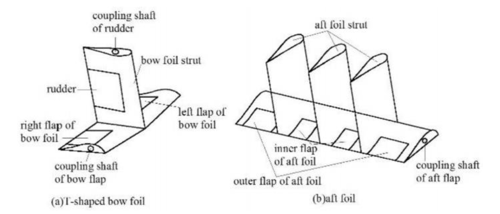
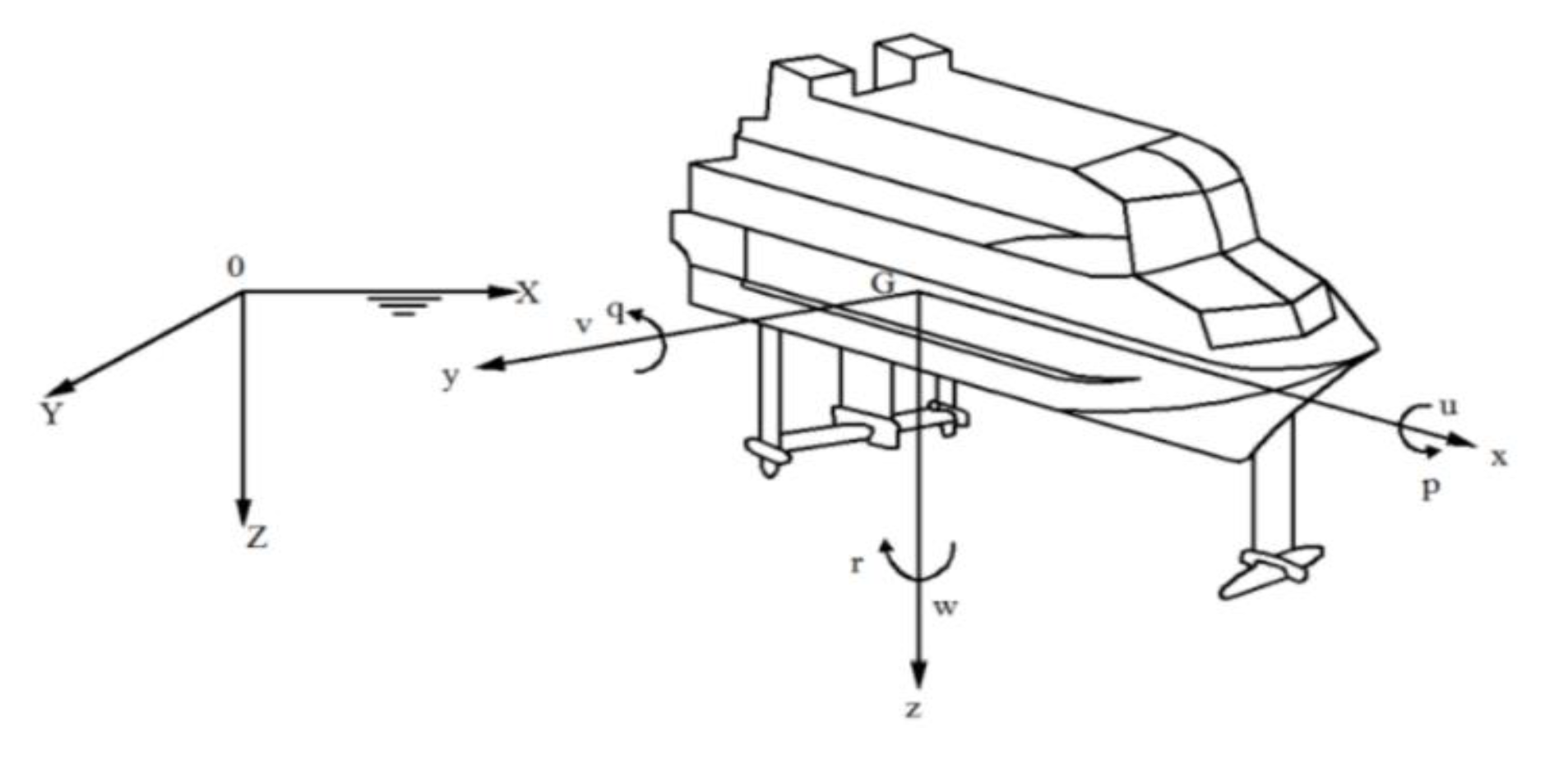
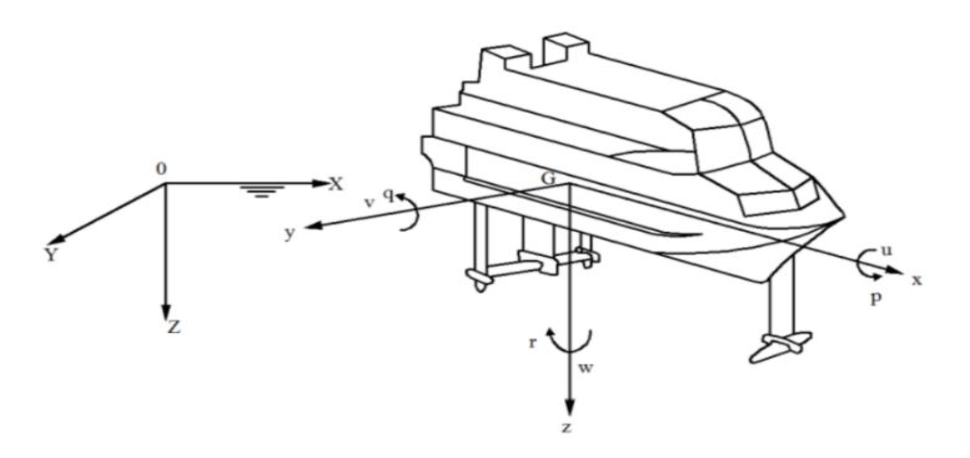
2.1. Construction of Longitudinal Model of Hydrofoil Craft

Hydrofoil craft is composed of four parts: hull, hydrofoil, propulsion system and control system. This article is based on PCH-1 made in the United States [23,24]. It is a fully submersible seaplane designed by the United States, which is suitable for marine conditions and meets military standards. The duckbill configuration is adopted and a control flap is used to control the heave of the fully submerged hydrofoil craft. A hydrofoil with a larger aspect ratio is used as the rear hydrofoil to provide more lift. The control flap is connected to it to control the pitch and heave attitude together with the front flap. The three views of the hydrofoil craft model and the hydrofoil-flap assembly drawing used are shown in Figure 2 and Figure 3 respectively.

In order to comprehensively study the motion of a ship, it is necessary to establish a fixed coordinate system and a moving coordinate system [25]. The coordinate system fixed on the earth is also called the fixed coordinate system, and O is the origin of the coordinate system fixed on the earth’s surface. The X-axis is in the still water plane, and it can usually be selected as the general motion direction of the ship. The Y-axis is selected as the direction in which the X-axis rotates clockwise in the hydrostatic plane. The Z-axis is perpendicular to the hydrostatic plane and points to the earth center. The coordinate system fixed to the ship is also called the moving coordinate system. The origin G of the coordinate system is usually taken at the center of gravity of the ship and moves with the ship. The x-axis is taken as the longitudinal section perpendicular to the midship and pointing to the bow. The y-axis is perpendicular to the midship cross section and points to the right chord. The z-axis is perpendicular to the waterline plane and points to the keel. In ship motion, there are usually six degrees of freedom, of which three degrees of freedom are longitudinal motions, namely, surge, pitch and heave. This article mainly studies pitch and heave, and does not consider surge. As shown in Figure 4, it is the coordinate system of fully submerged hydrofoil craft.

Because of the irregularity of the hull shape and the randomness of the sea state, the hydrofoil craft is assumed to move in an infinite uniform flow field. The mathematical expressions of heave and pitch are as follows [26]:

$$\{\begin{array}{c}m(\ddot{h}+U_e\dot{\theta })=Z_f+Z_c+Z_w\\ I_{yy}\ddot{\theta }=M_f+M_c+M_w\end{array}$$

(1)

where m is the mass of the hydrofoil craft, h is the heave displacement, U_e is the ship speed, θ is the pitch angle, Z_f, M_f is the lift and moment of the hydrofoil, Z_c, M_c is the control force and control moment, and Z_w, M_w is the disturbance force and disturbance moment of the sea wave. The expansion of formula (1) can be written as follows:

$$\{\begin{array}{c}m(\ddot{h}+U_e\dot{\theta })={\displaystyle \sum _{i=1}^2(F_{fi}+F_{fpi})+mg\cos \theta +Z_w}\\ I_{yy}\ddot{\theta }=-{\displaystyle \sum _{i=1}^2(x_{fi}-x_G)(F_{fi}+F_{fpi})+M_w}\end{array}$$

(2)

where F_fi is the force generated by the hydrofoil, I_yy is the moment of inertia of the hull, and x_fi, x_G is the distance from the hydrofoil and the center of gravity to the center of the ship. The symbol of x_fi, x_G is determined by the position of the relative stress action point in the ship. The “+” sign is taken before and “−” sign is taken after. When i = 1, it is related to the front wing, and i = 2, it is related to the rear wing.

Then rewrite the above formula into the following form to obtain:

$$\{\begin{array}{c}Z(\ddot{h},\dot{h},h,\ddot{\theta },\dot{\theta },\theta )=m(\ddot{h}+U_e\dot{\theta })-{\displaystyle \sum _{i=1}^2(F_{fi}+F_{fpi})-mg\cos \theta -Z_w=0}\\ M(\ddot{h},\dot{h},h,\ddot{\theta },\dot{\theta },\theta )=I_{yy}\ddot{\theta }+{\displaystyle \sum _{i=1}^2(x_{fi}-x_G)(F_{fi}+F_{fpi})-M_w=0}\end{array}$$

(3)

Linearize the left end of the equation and substitute the parameters of PCH hydrofoil craft to obtain:

$$\{\begin{array}{c}{Z}_{\ddot{h}}\ddot{h}+Z_{\dot{h}}\dot{h}+Z_{h}h+Z_{\ddot{\theta }}\ddot{\theta }+Z_{\dot{\theta }}\dot{\theta }+Z_{\theta }\theta =-Z_{\delta }{}_{{}_e}{\delta }_e-Z_{\delta }{}_f{\delta }_f-Z_w\\ M_{\ddot{h}}\ddot{h}+M_{\dot{h}}\dot{h}+M_{h}h+M_{\ddot{\theta }}\ddot{\theta }+M_{\dot{\theta }}\dot{\theta }+M_{\theta }\theta =-M_{\delta }{}_{{}_e}{\delta }_e-M_{\delta }{}_f{\delta }_f-M_w\end{array}$$

(4)

$$\{\begin{array}{c}\ddot{h}+6.06h+0.338h+3.41\ddot{\theta }+42.4\dot{\theta }+454\theta =-51.5{\delta }_e-62.9{\delta }_f-Z_w\\ 0.016\ddot{h}+0.069\dot{h}+\ddot{\theta }+8.45\dot{\theta }+0.654\theta =4.58{\delta }_e-1.88{\delta }_f-M_w\end{array}$$

(5)

In modern control theory, state feedback and matrix operation are adopted to convert the above differential equation into the form of state equation, so the continuous state equation of longitudinal motion is:

$$\left[\begin{array}{c}\ddot{h}\\ \ddot{\theta }\end{array}\right]=\left[\begin{array}{cccc}-0.6079& -6.412& -478.024& -14.3747\\ 0.0791& 0.1033& 7.0452& -8.2187\end{array}\right]\left[\begin{array}{c}\begin{array}{l}h\\ \dot{h}\end{array}\\ \begin{array}{l}\theta \\ \dot{\theta }\end{array}\end{array}\right]+\left[\begin{array}{cc}-71.016& -59.7706\\ 5.7234& -0.9177\end{array}\right]\left[\begin{array}{c}{\delta }_e\\ {\delta }_f\end{array}\right]+\left[\begin{array}{cc}1.0577& -3.6069\\ 0.017& 1.0577\end{array}\right]\left[\begin{array}{c}{Z}_w\\ M_w\end{array}\right]$$

(6)

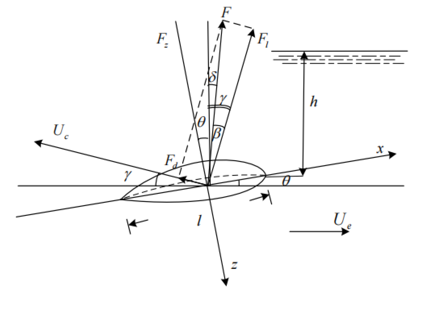
2.2. Force analysis of Hydrofoil

The hydrofoil installed at the bottom is the biggest difference between hydrofoil crafts and other ships, which is the key to ensure its stable navigation. When traveling at a certain speed, the pressure difference caused by the flow velocity difference between the upper and lower hydrofoil plates will generate buoyancy, which will make the hull come completely out of the water, reduce the resistance, improve the speed, and provide better stability. The plane geometric structure and wing section structure of the hydrofoil are shown in Figure 5 and Figure 6.

In Figure 5, where b is the wingspan, l_r is the tip chord, l_t is the root chord, the average chord length is l, and the aspect ratio is λ= b/l. In Figure 6, the section along the inflow direction is called the wing section. The foremost point LE on the wing section is the leading edge, and the rearmost point TE is the trailing edge. AB is the maximum thickness of the wing section and the distance from AB to the leading edge is x_c. The longest line segment CD is the maximum camber, and the distance from CD to the leading edge is x_f.

Next, the force analysis is carried out. The characteristic that the hydrofoil can generate lift is also called the hydrodynamic characteristic. The complete force analysis of the hydrofoil during the navigation of the hydrofoil craft is shown in Figure 7 [27].

In the figure, F is the resultant force of the hydrofoil, F_l is the lift of the hydrofoil, and F_d is the resistance of the hydrofoil. δ is the angle between the resultant force and the vertical line of the water surface, θ is the angle between the hydrofoil plane and the horizontal direction, β is the angle between the lift force and the resultant force, γ is the angle between the lift and the vertical water surface line. Lift, drag and lift drag ratio can be expressed as follows:

$$F_l=\frac{1}{2}{C}_L\rho U_e{}^{2}S$$

(7)

$$F_d=\frac{1}{2}{C}_D\rho U_e{}^{2}S$$

(8)

$$K=\frac{F_l}{F_d}=\frac{C_L}{C_D}$$

(9)

where ρ is the sea water density, U_e is the ship speed, and S = l·b is the area of the hydrofoil. Among them, the lift drag ratio K is one of the important parameters reflecting the performance of the hydrofoil, and it is the ratio of the lift coefficient and the drag coefficient. The lift coefficient can be obtained by two methods of test or calculation according to the hydrofoil theory. Generally, it is assumed that the thickness, camber and angle of attack of the airfoil section are small and the airfoil is deep from the water surface. The formula is as follows:

$$C_L=2\pi (\alpha +\frac{2f}{l})$$

(10)

where α is the attack angle of the hydrofoil and f is the camber. When the camber coefficient of the thin wing of the plate is approximately 0, the lift coefficient is obtained C_L = 2πα.

The flap is the part that provides stable control force for the longitudinal movement of the hydrofoil craft. The control force formula generated by the flap is as follows:

$$F_f=\frac{1}{2}{C}_{Lf}\rho U_e{}^2{S}_f{\alpha }_f$$

(11)

where, S_f is the area of the flap, α_f is the angle of attack of the flap, C_Lf is the lift coefficient of the flap, and its calculation method is similar to that of the hydrofoil. However, due to the limitation of the mechanical structure, the lift coefficient of the flap is linear within a certain angle, so the flap servo system needs to set the maximum angle to ensure the appropriate control force of the hydrofoil craft.

Since the waves have great randomness and complexity in time and space, they can be considered to be formed by the superposition of multiple regular waves with different wavelengths, frequencies, wave amplitudes, phases and propagation directions, and then the disturbance force and moment are analyzed. The irregular wave model is as follows:

$$\xi ={\displaystyle \sum _{i=1}^{\mathrm{n}}{A}_i\cos ({\omega }_{ei}t+{\epsilon }_i+{\psi }_i)}$$

(12)

where n = 50, ε_i is the ith phase randomly generated on [0, 20], and the formula of wave amplitude A_i and encounter frequency ω_ei is as follows:

$$A_i={(2S({\omega }_i)△\omega )}^{\frac{1}{2}}$$

(13)

$${\omega }_{ei}=(\frac{2\pi }{{\lambda }_i})(U_R\cos \chi -c)$$

(14)

$${\psi }_i=(\frac{2\pi }{{\lambda }_i})(x\cos \chi +y\sin \chi )$$

(15)

$${\omega }_i=\frac{2\pi c}{{\lambda }_i}$$

(16)

where, S(ω_i) is the P-M spectrum, λ_i is the wavelength, c is the wave velocity, χ is the encounter angle, and ω_i is the actual frequency. In this article, the P-M spectrum used in the research of ship hull, which is currently popular internationally, is used for analysis. The spectral density function is as follows [28].

$$S(\omega )=\frac{A}{{\omega }^5}{e}^{-\frac{B}{{\omega }^4}}$$

(17)

A = 8.1 × 10⁻³ g², B = 3.11/H_1/3², H_1/3 is significant wave height, and Figure 8 is the curve under different significant wave heights.

After analysis and collation, it is concluded that the forces and moments generated by irregular waves on the hydrofoil are:

$$Z_2={\displaystyle \sum _{i=1}^{\mathrm{n}}{F}_{\mathrm{z}i}\cos ({\omega }_{ei}t+{\varphi }_{zi}+{\epsilon }_i)}$$

(18)

$$M_2={\displaystyle \sum _{i=1}^{\mathrm{n}}{M}_{ei}\cos ({\omega }_{ei}t+{\varphi }_{Mi}+{\epsilon }_i)}$$

(19)

where:

$$F_{\mathrm{z}i}=2\pi U_R{A}_{i}c/{\lambda }_i{e}^{-2\pi z/{\lambda }_i}{[{(K_b\cos {\psi }_{bi}+K_f\cos {\psi }_{fi})}^2+{(K_b\sin {\psi }_{bi}+K_f\sin {\psi }_{fi})}^2]}^{\frac{1}{2}}$$

(20)

$$K_b=(1/2)\rho U_R{}^2{A}_{fb}{\left(\partial C_L/\partial \alpha \right)}_b$$

(21)

$${\psi }_{bi}=(2\pi X_b/{\lambda }_i)\cos \chi$$

(22)

$$K_f=(1/2)\rho U_R{}^2{A}_{ff}{\left(\partial C_L/\partial \alpha \right)}_f$$

(23)

$${\psi }_{fi}=(-2\pi /{\lambda }_i)(L_s-X_b)\cos \chi$$

(24)

$${\varphi }_{zi}=\arctan (-\frac{K_b\cos {\psi }_{bi}+K_f\cos {\psi }_{fi}}{K_b\sin {\psi }_{bi}+K_f\sin {\psi }_{fi}})$$

(25)

$$\begin{array}{ll}{M}_{ei}& =2\pi U_R{A}_{i}c/{\lambda }_i{e}^{-2\pi z/{\lambda }_i}[{(-X_b{K}_b\cos {\psi }_{bi}+(L_s-X_b)K_f\cos {\psi }_{fi})}^2\\ & +{(-X_b{K}_b\sin {\psi }_{bi}+(L_s-X_b)K_f\sin {\psi }_{fi})}^2{]}^{\frac{1}{2}}\end{array}$$

(26)

$${\varphi }_{Mi}=\arctan [-\frac{-X_b{K}_b\cos {\psi }_{bi}+(L_s-X_b)K_f\cos {\psi }_{fi}}{-X_b{K}_b\sin {\psi }_{bi}+(L_s-X_b)K_f\sin {\psi }_{fi}}]$$

(27)

where, X_b is the distance from the center of gravity of the hull to the front hydrofoil, and L_s is the distance between the front and rear hydrofoils. It should be noted that when the encounter frequency ω_ei is negative, the minus sign before Equations (25) and (27) should be removed to calculate φ_zi and φ_Mi.

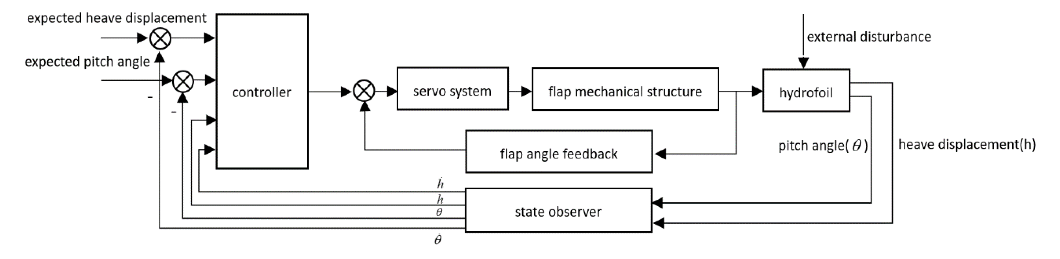
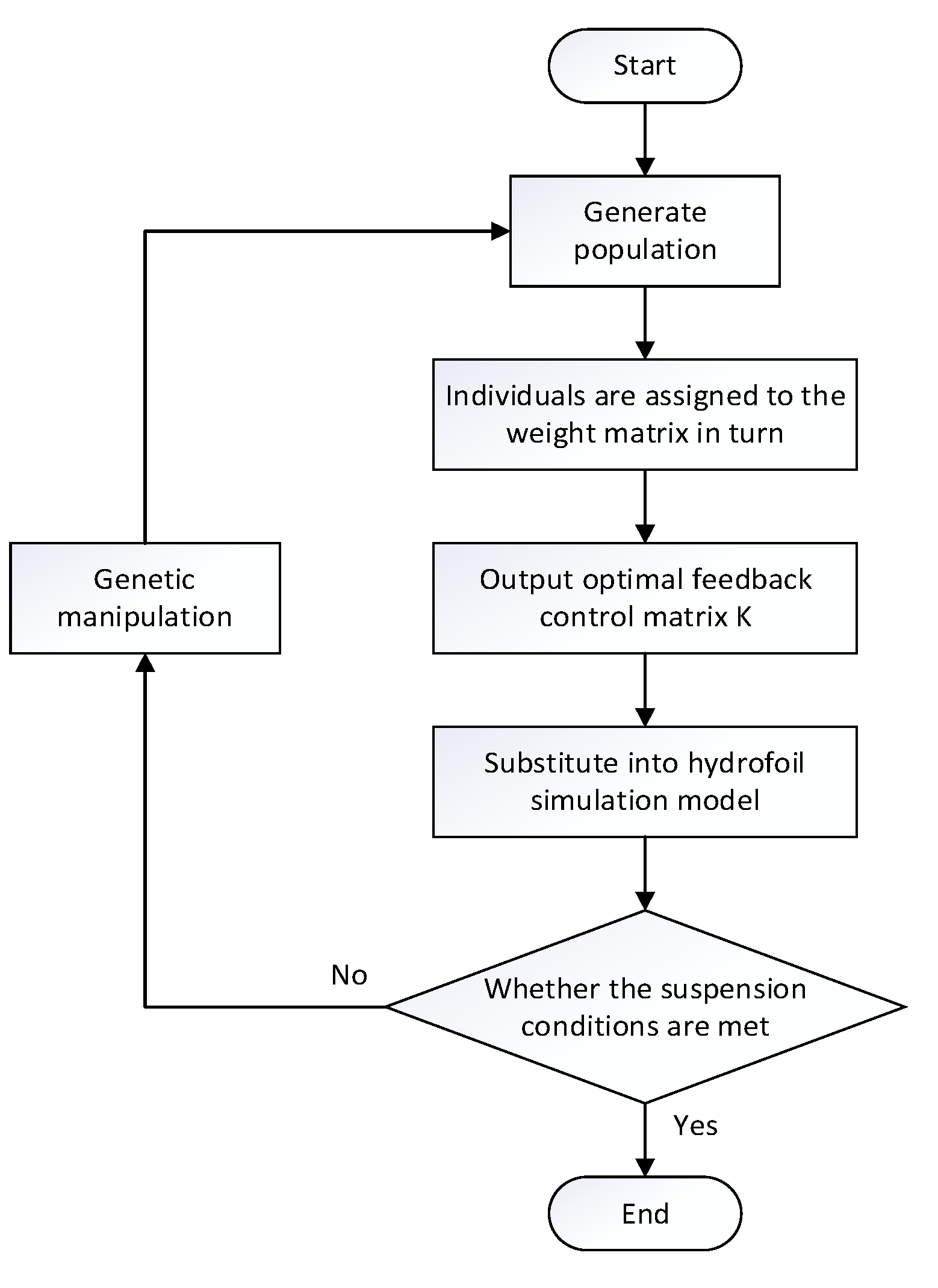
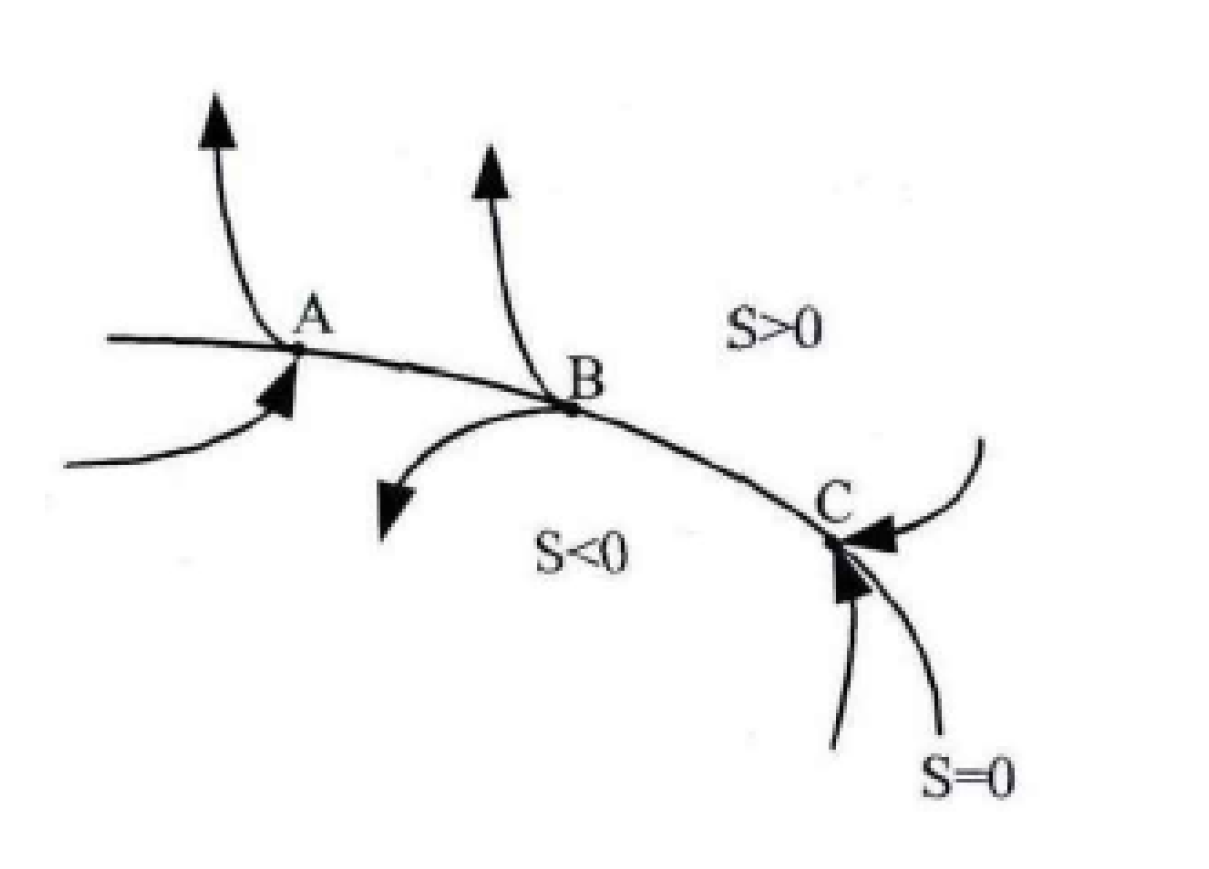
3. Design of Longitudinal Motion Controller of Hydrofoil Based on LQR/LQRY-SMC

The control system has a very important role in the stable navigation of the hydrofoil craft, and is also the focus of this article. According to the changes of the sea conditions, the flap angle is adjusted to generate the required restoring force and restoring moment, reduce the longitudinal motion of the full-submerged hydrofoil craft, and realize the stabilization of the longitudinal motion attitude of the full-submerged hydrofoil craft. Generally, a closed loop is composed of the controlled object (hull), sensor, controller and actuator. The state observer is used to obtain the required state value. The controller gives the flap-command angle signal according to the attitude angle and displacement to reduce the deviation between the actual value and the expected value. The actuator is mainly composed of the servo system, the flap-mechanical structure and the flap-angle feedback measurement device. Figure 9 is a block diagram of the control system.

The joint control in this article first needs to analyze the LQR control part. This method is easy to realize, and the optimal control law of state-linear feedback can be obtained. At the same time, the original system can achieve a better performance index with low cost. The performance index function J(u) needs to be defined to have a minimum value.

$$J(u)=\frac{1}{2}{x}^T(T)S(T)x(t)+\frac{1}{2}{\displaystyle {\int }_0^T(x^T(t)Q(t)x(t)+u^T(t)R(t)u(t))}dt$$

(28)

The Q and R matrices are used to adjust the input variables and state variables of the cost function to find the optimal value. If not only the influence of system state x(t) and control quantity u(t) is considered, but also the output quantity y(t) is introduced, it can be called LQ optimal control based on output regulation, also called LQRY control.

$$J(u)=\frac{1}{2}{x}^T(T)S(T)x(t)+\frac{1}{2}{\displaystyle {\int }_0^T(x^T(t)Q(t)x(t)+u^T(t)R(t)u(t)+y^T(t)F(t)y(t))}dt$$

(29)

The optimal feedback gain matrix of LQR/LQRY can be expressed as:

$$u(t)=-R^{-1}{B}^{T}Px(t)$$

(30)

$$K=-R^{-1}{B}^{T}P$$

(31)

where P is the solution of Riccati equation, the equation is as follows:

$$PA+A^{T}P+Q-PB{R}^{-1}{B}^{T}P=0$$

(32)

$$PA+A^{T}P+Q+C^{T}FC-PB{R}^{-1}{B}^{T}P=0$$

(33)

The above control mode can also use some optimization algorithms to further reduce the longitudinal motion of the hydrofoil craft. In this article, the genetic algorithm is used to select the appropriate fitness function to optimize the Q and R matrix [29]. The process diagram is shown in Figure 10.

Then analyze the sliding mode control part, let a system be: $\dot{x}=f(x),x\in R^n$, there is a plane $s(x)=s(x_1,x_2,\dots ,x_n)=0$, as shown in Figure 11.

As can be seen from the figure, this plane divides the state space into two parts. Once the moving point in the state space enters the plane range during the movement, there are three different states, namely, the normal point A, the starting point B and the ending point C. In order to keep the system stable, it is desirable that the motion point in the plane range be the termination point, because other motion points in the state space will become the constant motion of the termination point in the region when they enter the plane range, so this region is called the sliding-mode region. From the sliding-mode analysis, it needs to meet the following requirements: $\underset{s\to 0}{\lim s\dot{s}}\le 0$.

According to formula (6), the hydrofoil craft can be regarded as the following second-order uncertain nonlinear dynamic system:

$$\{\begin{array}{l}{\dot{x}}_1=x_2\\ {\dot{x}}_2=f(x)+g(x)+b(x)u\end{array}$$

(34)

f(x), g(x) and b(x) can be determined by formula (6) to obtain:

$$f(x)=\left[\begin{array}{cccc}-0.6079& -478.024& -6.4120& -14.3747\\ 0.0791& 7.0452& 0.1033& -8.2187\end{array}\right]\left[\begin{array}{c}h\\ \dot{h}\\ \theta \\ \dot{\theta }\end{array}\right]$$

(35)

$$b(x)=\left[\begin{array}{cc}-71.016& -59.7706\\ 5.7234& -0.9177\end{array}\right]$$

(36)

$$g(x)=\left[\begin{array}{cc}1.0577& -3.6069\\ 0.017& 1.0577\end{array}\right]\left[\begin{array}{c}{Z}_w\\ M_w\end{array}\right]$$

(37)

According to the characteristics of the fully submerged hydrofoil craft, the sliding-mode function selected by the sliding mode variable structure control part in this article is as follows:

$$s=x_1+\frac{1}{\beta }{x}_2{}^{p/q}$$

(38)

where β > 0, p > q, p and q are positive odd numbers. The sliding-mode controller designed according to the linearization feedback theory is:

$$u=-b^{-1}(x)\left(f(x)+\beta \frac{q}{p}{x}_2{}^{2-p/q}+0.1\mathrm{sgn}(s)\right)$$

(39)

Its stability is proved as follows:

$$\begin{array}{l}\dot{s}={\dot{x}}_1+\frac{p}{\beta q}{x}_2{}^{p/q-1}{\dot{x}}_2\\ =x_2+\frac{p}{\beta q}{x}_2{}^{p/q-1}[f(x)+g(x)+b(x)u]\\ =\frac{p}{\beta q}{x}_2{}^{p/q-1}(g(x)-0.1\mathrm{sgn}(s))\end{array}$$

(40)

Multiply both sides by s:

$$s\dot{s}=\frac{p}{\beta q}{x}_2{}^{p/q-1}(sg(x)-0.1\left|s\right|)$$

(41)

Because $1<p/q<2$, then $0<p/q-1<1$, $x_2{}^{p/q-1}>0$, it can be proved that

$$s\dot{s}\le -\frac{0.1p}{\beta q}{x}_2{}^{p/q-1}\left|s\right|$$

(42)

Because $-0.1p/\beta q*x_2{}^{p/q-1}\le 0$, then $s\dot{s}\le 0$, the controller satisfies the Lyapunov stability condition. In order to further enhance the control effect, it is considered to combine the above two control methods to form LQRY-SMC. The controller formula is as follows:

$$u=-Kx-b^{-1}(x)\left(f(x)+\beta \frac{q}{p}{x}_2{}^{2-p/q}+0.1\mathrm{sgn}(s)\right)$$

(43)

4. Design of Longitudinal Motion Controller of Hydrofoil Based on LQR/LQRY-SMC

The simulation in this section firstly needs to substitute the disturbance force and disturbance moment under irregular wave waves with different parameters into the formula in Section 2.2, and then substitute the data results into the controller simulation as the external disturbance part. Under different wave heights, the LQRY and sliding-mode control alone and the LQRY-SMC using them together are simulated and the data diagram is obtained.

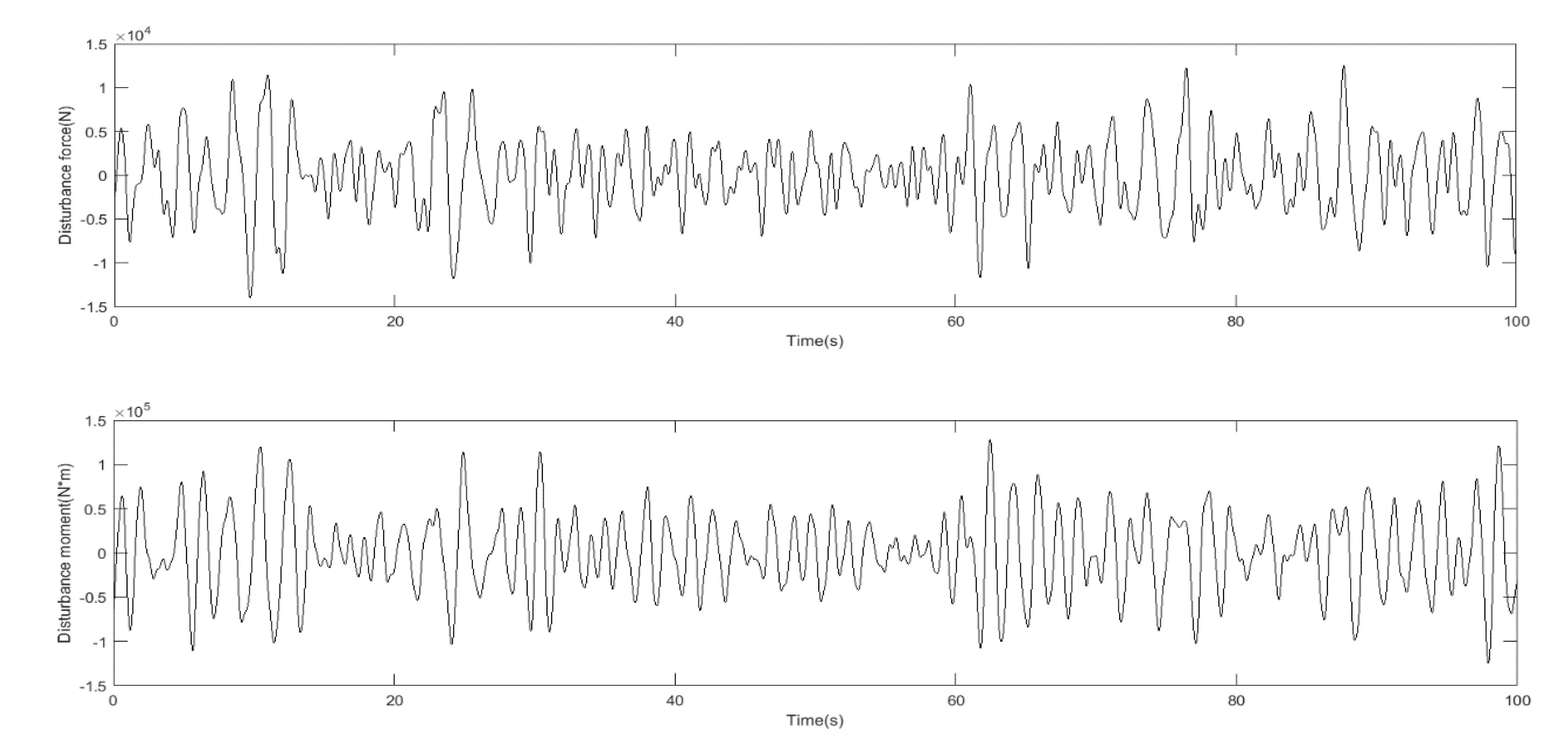
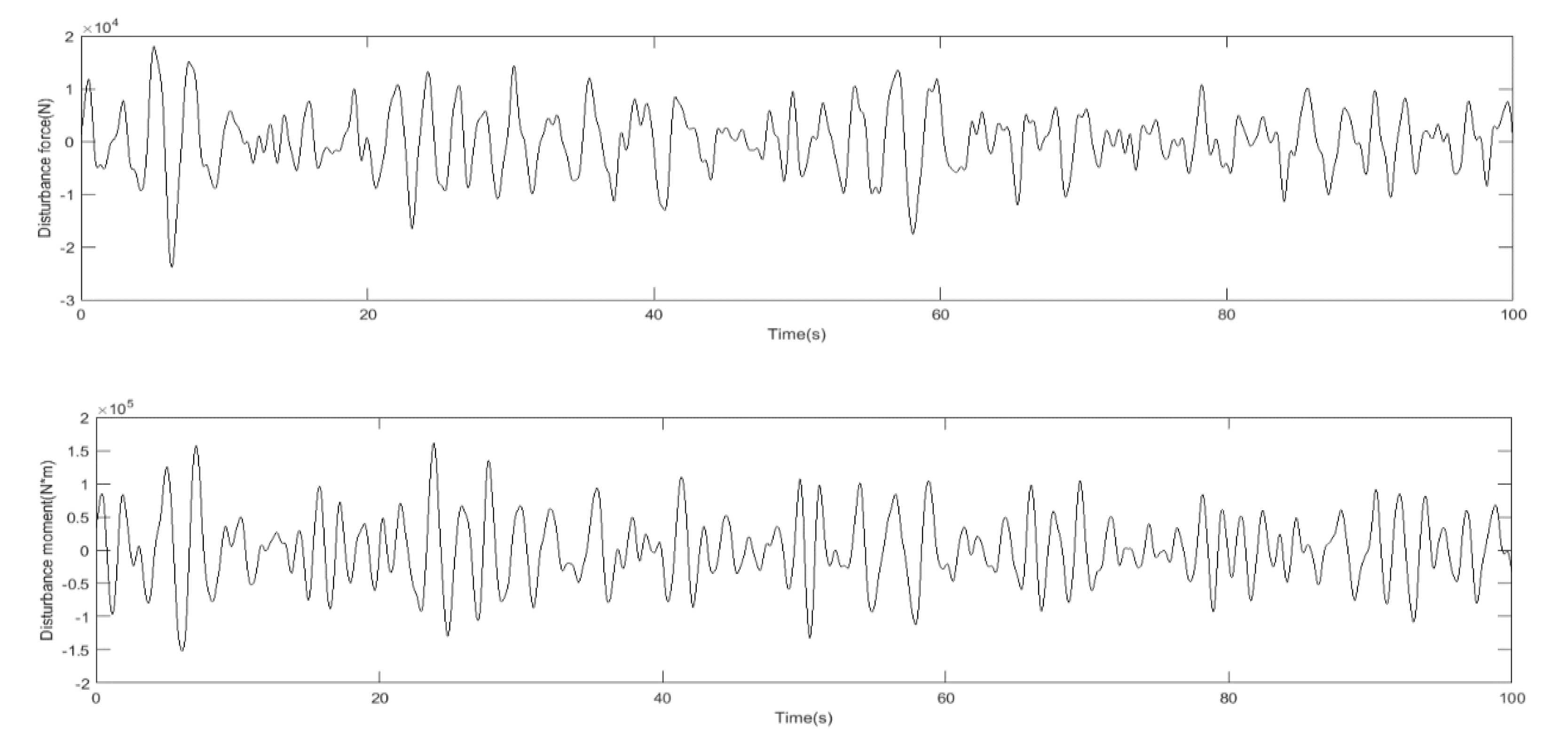
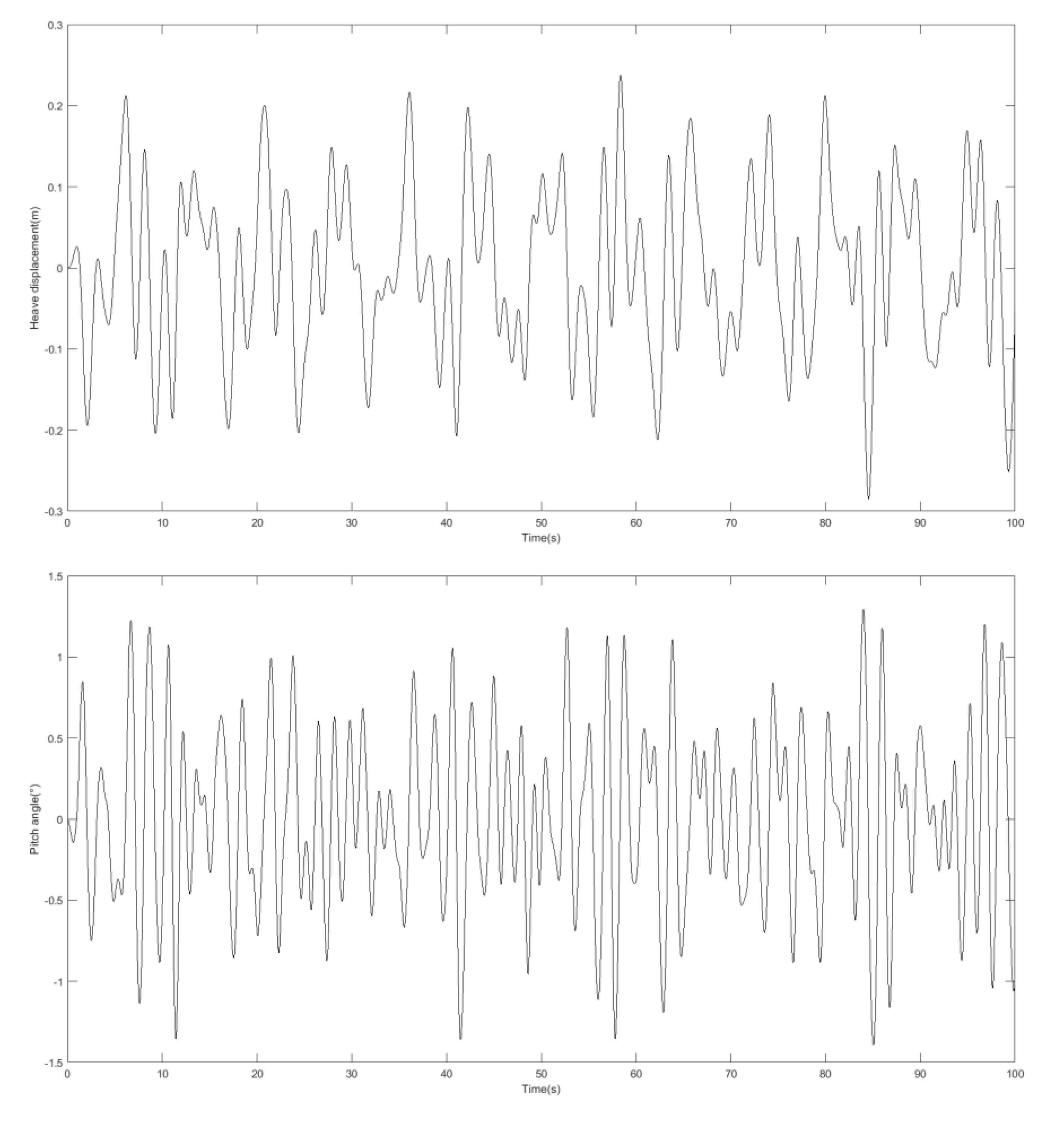
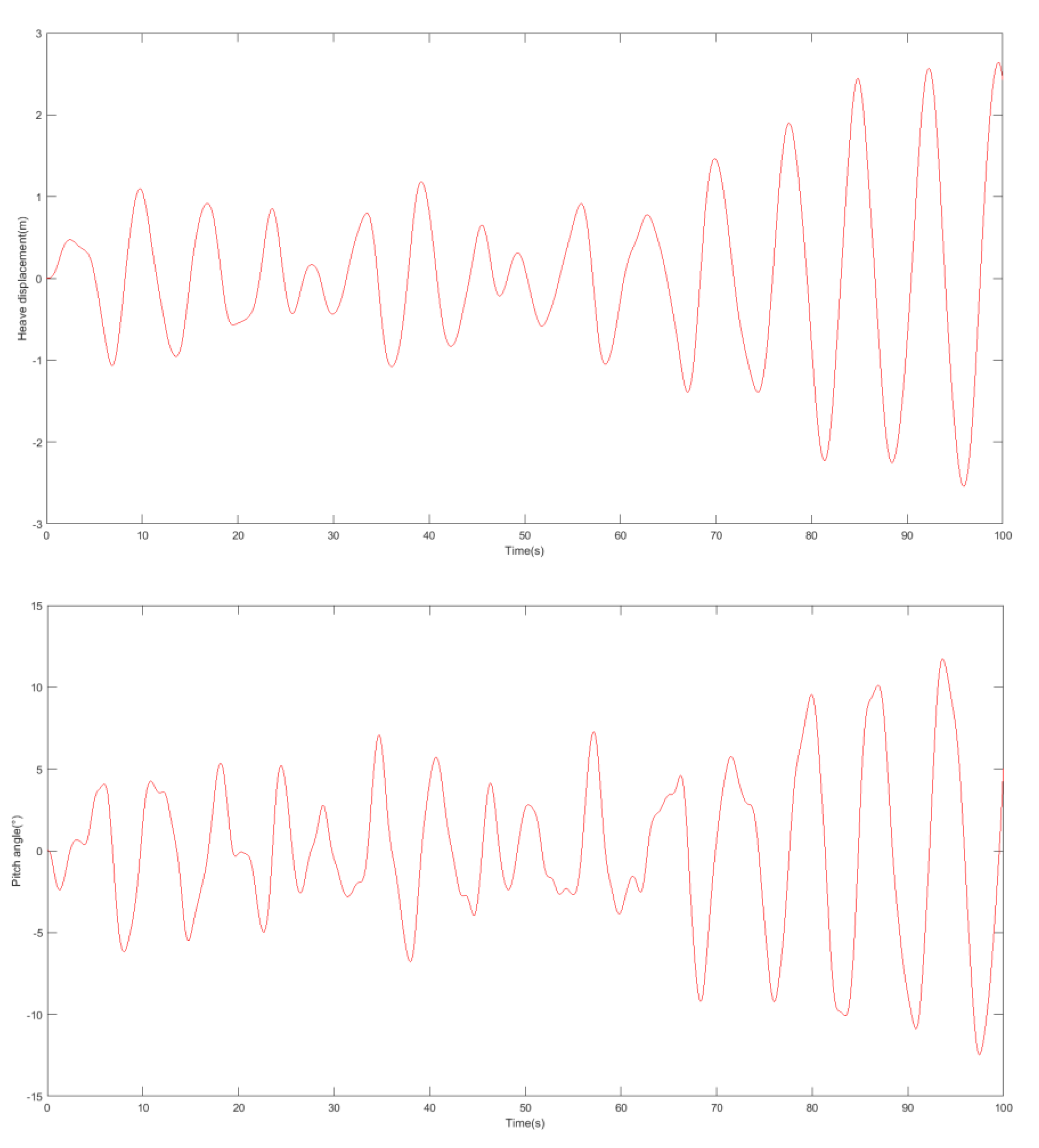
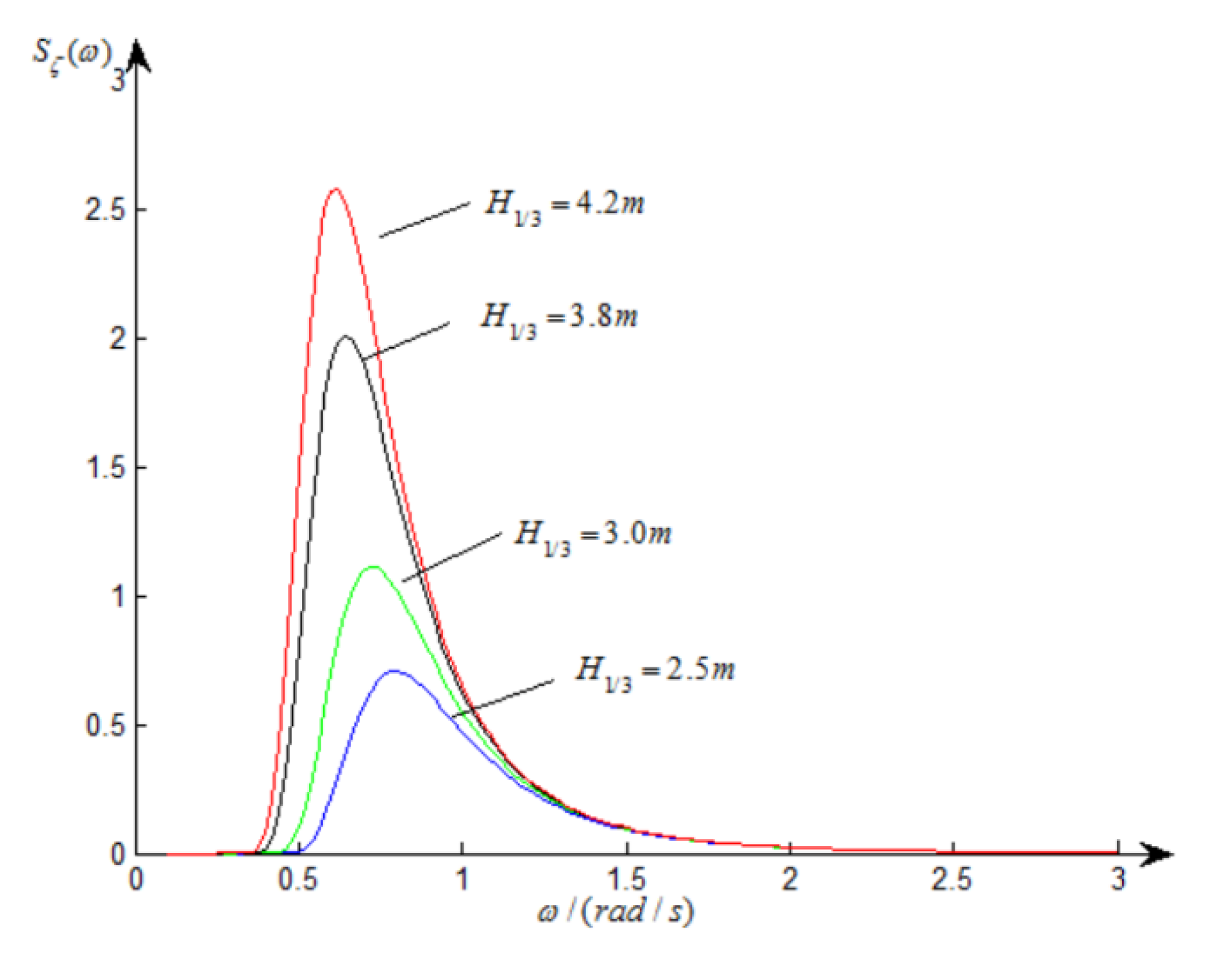
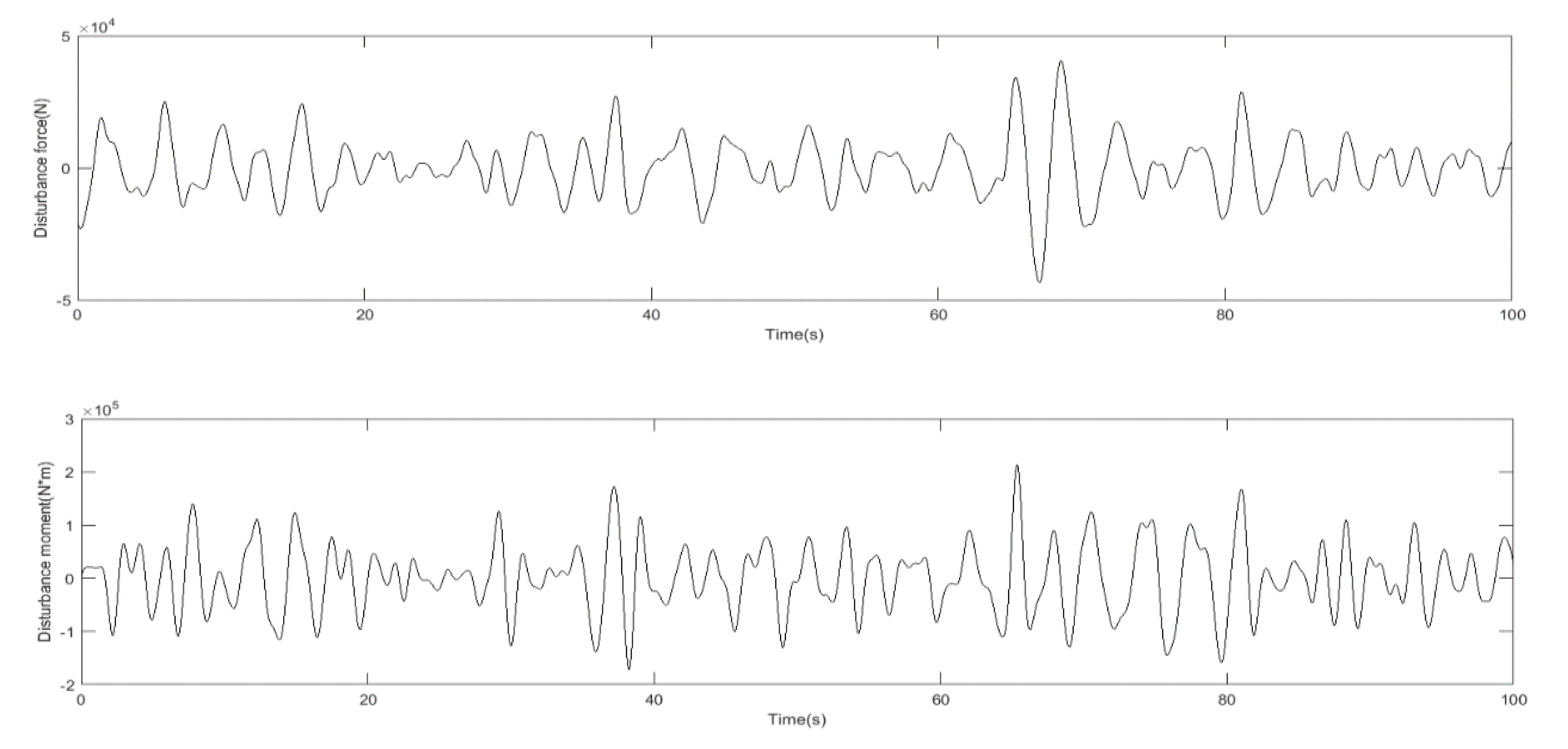
4.1. Simulation of Disturbance Force and Moment

In order to more intuitively show the disturbance effect of the hydrofoil craft by the sea waves, the ship model is used as a reference to simulate the disturbance force and moment of the ship under the action of random sea waves according to the above formula. The parameters of the hull model used are shown in

Table 1. Hydrofoil craft parameters.

Parameter	Symbolic Representation	Value	Unit
Craft weight	m	26,200	kg
Craft speed	Ue	35	kn
Average immersion depth	Z	1.52	m
Front hydrofoil area	Afb	6.08	m2
Rear hydrofoil area	Aff	13.90	m2
Distance from front hydrofoil to center of gravity	Xb	12.68	m
Distance between two hydrofoils	Ls	17.86	m

. The disturbance force and moment curves of 180° encounter angle and 1.5 m, 2 m, 3 m significant wave heights of the turbulent flow will be given in the article, as shown in Figure 12, Figure 13 and Figure 14.

It can be seen from the figure that the disturbance force of the hydrofoil craft is basically stable at 10⁴, and the disturbance moment is basically stable at 10⁵. The data results obtained here provide preconditions for the following control system simulation.

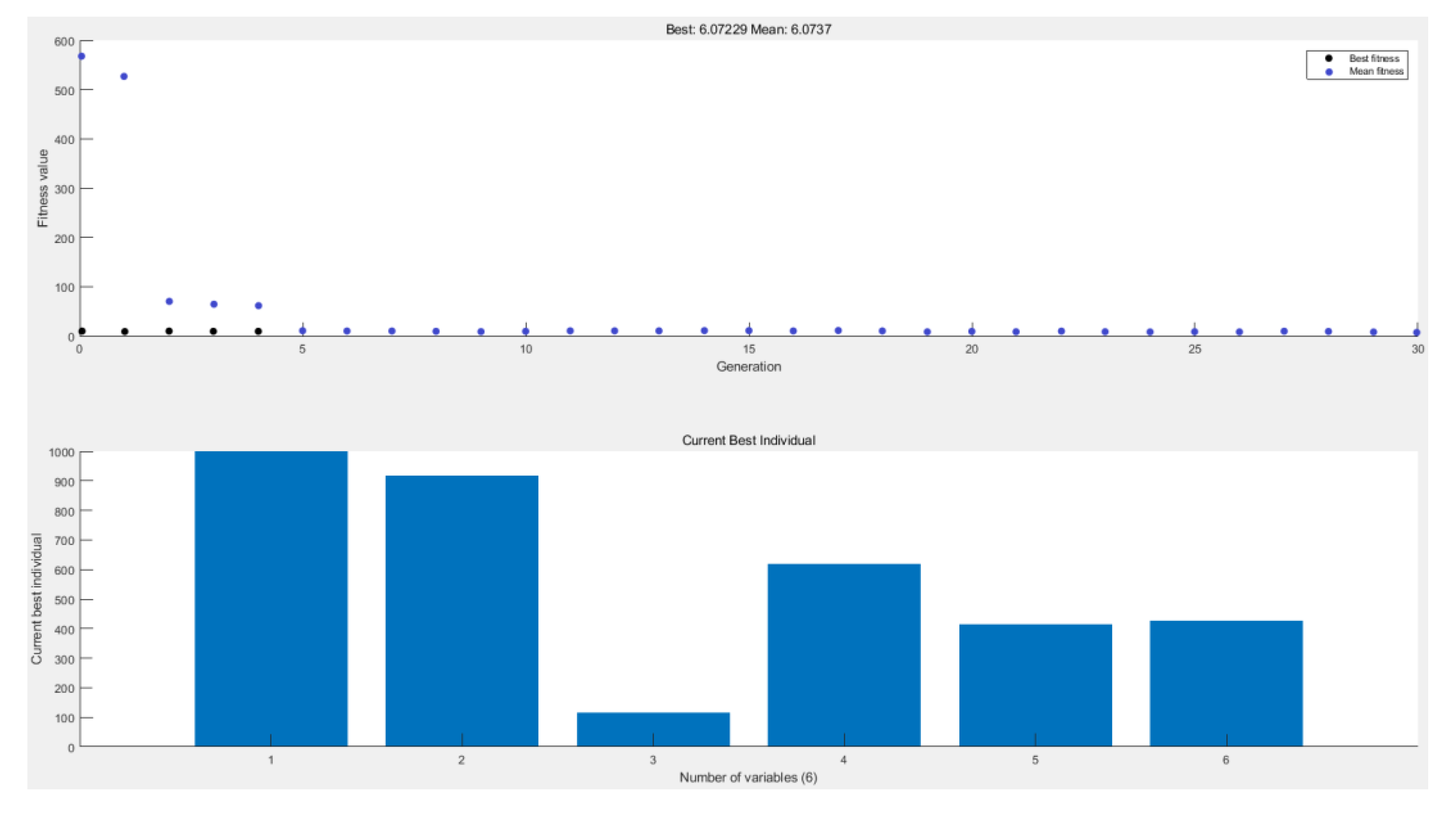
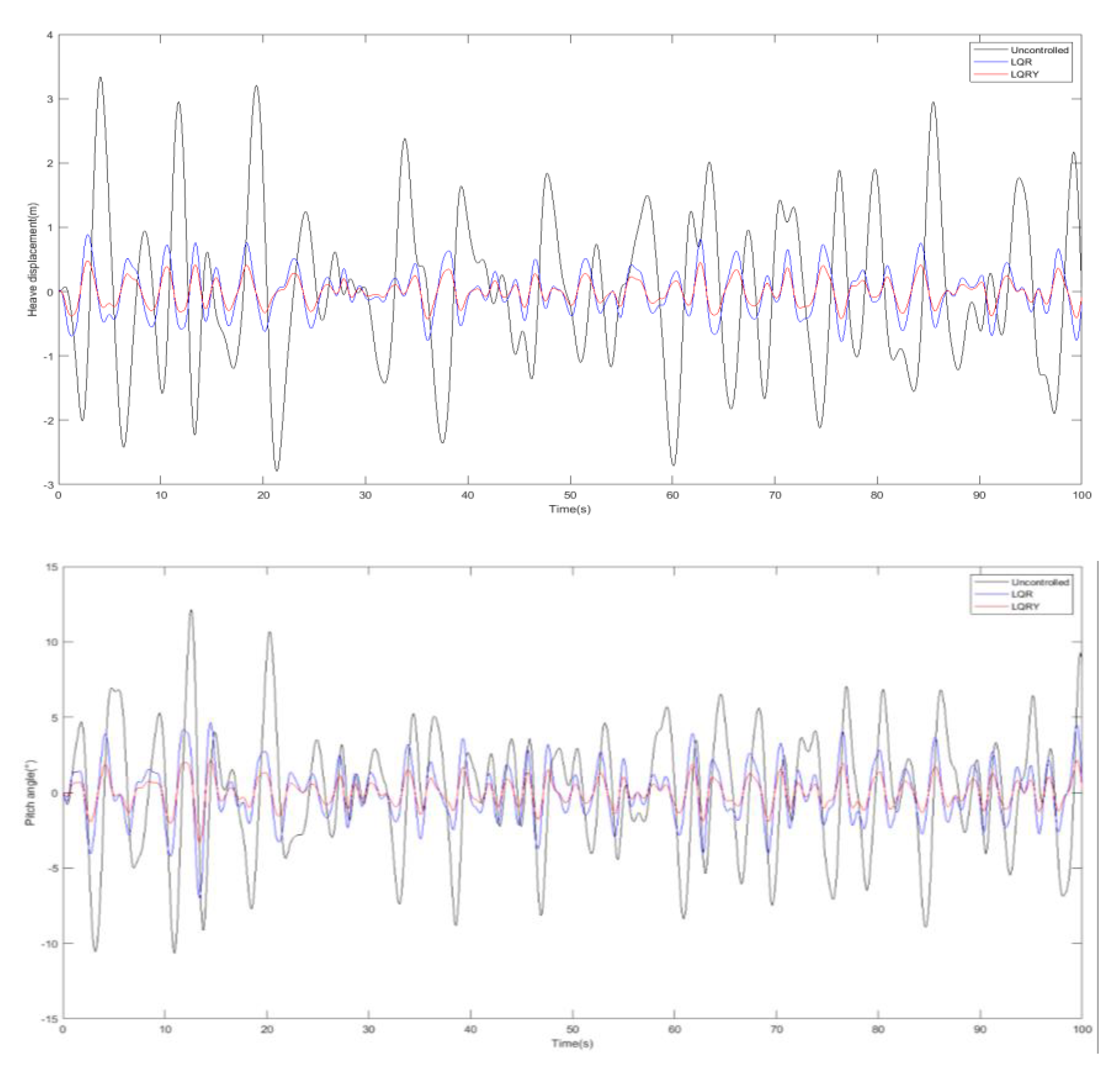
4.2. Comparative Simulation of Optimized LQR and LQRY Simulation

After the data of disturbance force and moment are obtained, the control performance of LQR and LQRY will be compared in this section. After comparison, the method more suitable for the next joint control will be selected to obtain better performance. The parameter table of optimization algorithm simulation is shown in

Table 2. Genetic algorithm parameters.

Parameter	Value
Initial population size	100
Number of elite individuals	10
Cross offspring ratio	0.75
Lower limit	[0.1 0.1 0.1 0.1 0.1 0.1]
Upper limit	[1000 1000 1000 1000 500 500]
Evolutionary algebra	30
Fitness function deviation	1e−100

, and the results are shown in Figure 15.

As can be seen from Figure 14, the result shows that the optimal fitness is 6.072, Q = diag [999.8614 918.9989 116.3479 618.8724], R = diag [415.6694 427.8040], and the value of K is:

$$Klqr=\left[\begin{array}{cccc}-1.1878& -1.0902& 5.8968& 0.5587\\ -0.9730& -0.9119& 0.9275& -0.3399\end{array}\right]Klqry=\left[\begin{array}{cccc}-1.1884& -1.0908& 5.8970& 0.5590\\ -0.9735& -0.9125& 0.9274& -0.3403\end{array}\right]$$

The simulation results of the longitudinal motion model substituted into the hydrofoil craft are shown in Figure 16 and

Table 3. Comparison results of uncontrolled, LQR, LQRY.

Control Method	hmax	E(h)	STD(h)	θmax	E(θ)	STD(θ)
Uncontrolled	3.3372	0.0036	1.2489	12.1330	0.0049	4.0937
LQR	0.8865	−0.0064	0.3535	4.6508	0.0236	1.8429
LQRY	0.4801	−0.0035	0.1930	2.1788	0.0113	0.8784

below:

In the specific case selected, it can be found that the optimized LQRY algorithm is better than the LQR algorithm in all indicators, in which the maximum-heave displacement and pitch angle are reduced by 45.8% and 53.2%, so the optimized LQRY will be used in the joint control with the sliding-mode algorithm.

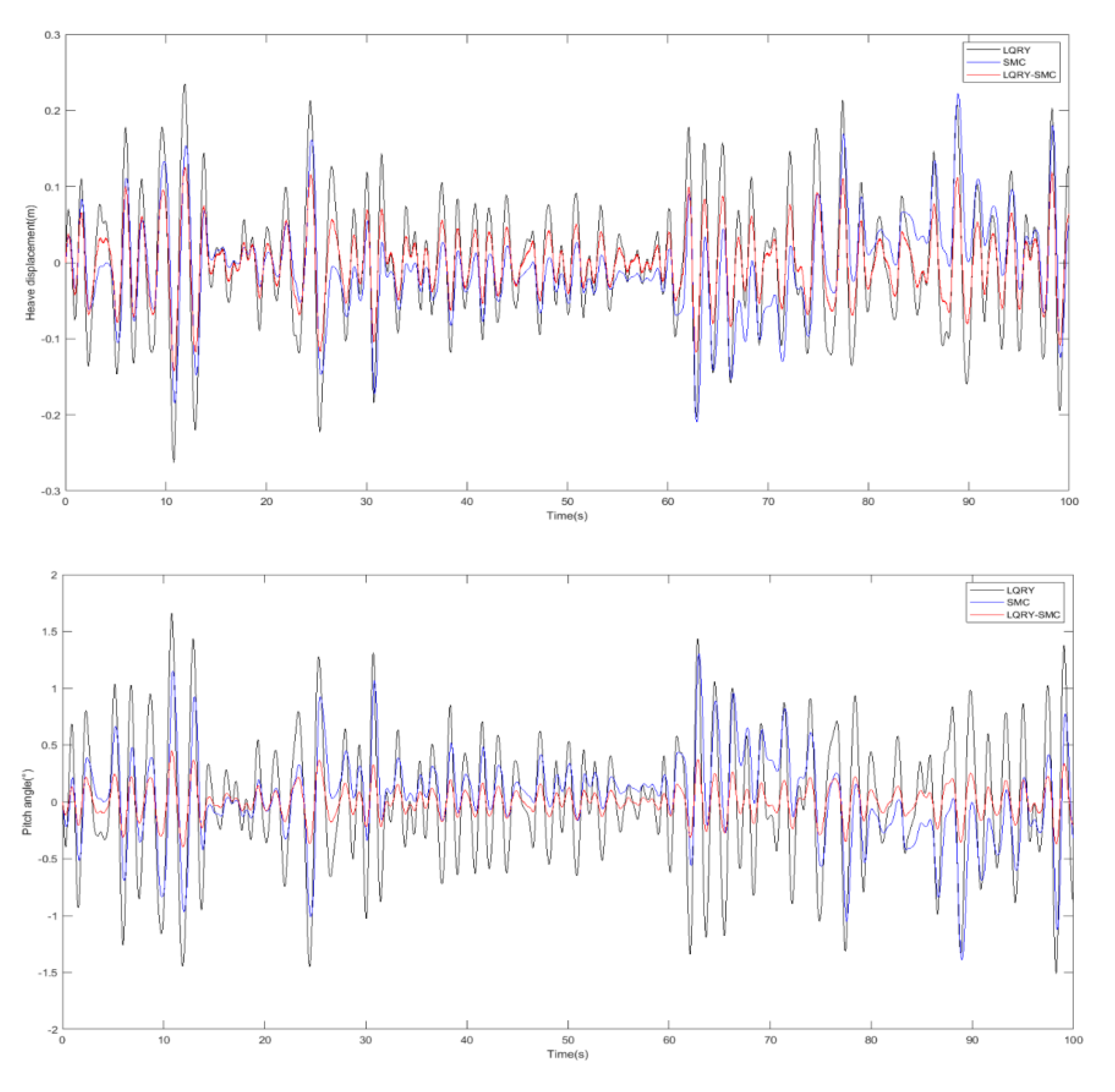
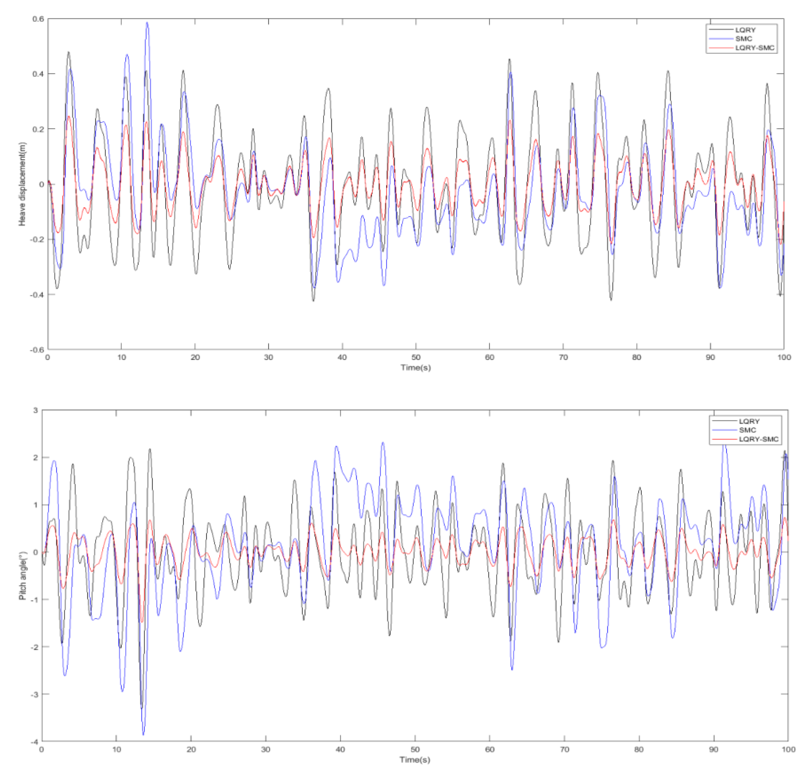
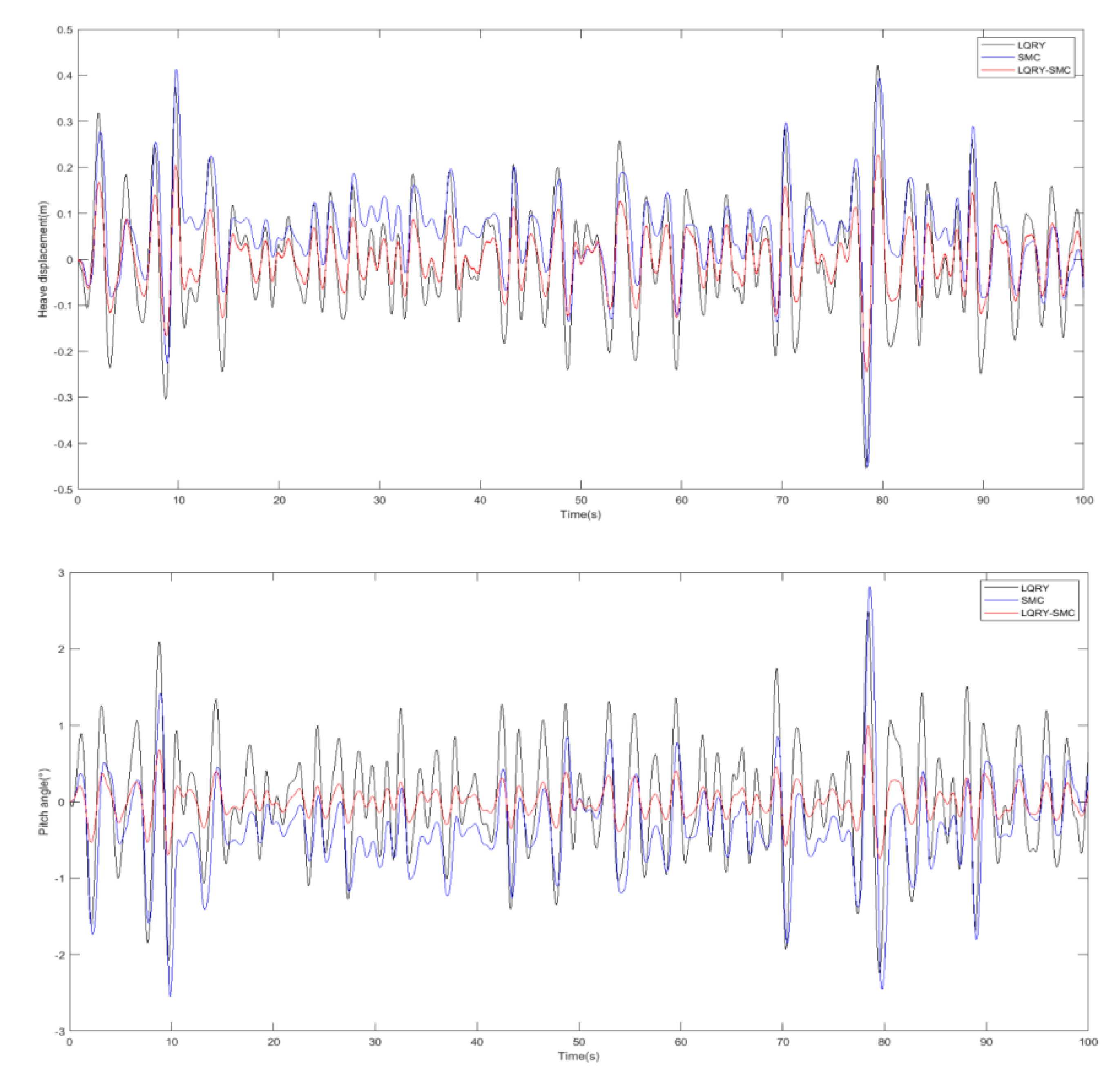
4.3. Comparative Simulation of LQRY, SMC and LQRY-SMC

After the superiority of LQRY is proved in the previous section, this section will verify the joint control and compare the heave displacement and pitch angle of LQRY and SMC alone. First of all, the control rate of the sliding mode control part shall be determined. It can be seen from Equation (39) that the parameter β, p, q shall be determined. In this article, β = diag [19.2 7.5], p = 7, q = 5.

In this section, in order to reflect the universality of joint control, to be applicable to a variety of complex sea conditions and to be more stable, the case of 180° encounter angle and 1.5 m, 2 m, 3 m significant wave heights of the turbulent flow are selected in the simulation. The simulation results are shown in Figure 17, Figure 18 and Figure 19, and the numerical values are arranged in

Table 4. Comparison results of LQRY, SMC, LQRY-SMC.

Wave Height	Control Method	hmax	E(h)	STD(h)	θmax	E(θ)	STD(θ)
1.5 m	LQRY	0.2625	1.9601 × 10−5	0.0814	1.6591	3.5457 × 10−4	0.5508
	SMC	0.2219	−0.0057	0.0611	1.3888	0.0355	0.3792
	LQRY-SMC	0.1429	−3.2011 × 10−4	0.0438	0.4515	9.4201 × 10−4	0.1386
2 m	LQRY	0.4552	8.6007 × 10−4	0.1221	2.4925	−8.4116 × 10−4	0.7204
	SMC	0.4506	0.0538	0.0949	2.8112	−0.3344	0.5907
	LQRY-SMC	0.2453	9.2481 × 10−4	0.0644	0.9975	−0.0019	0.2132
3 m	LQRY	0.4801	−0.0035	0.1930	3.3249	0.0113	0.8784
	SMC	0.5864	−0.0242	0.1673	3.8698	0.1399	1.0303
	LQRY-SMC	0.2462	−0.0026	0.0942	1.4875	0.0053	0.3173

.

It can be seen from the simulation curves from Figure 17 to Figure 19 that when the significant wave height is 3 m, the sliding-mode control is greatly affected by the high sea conditions and cannot effectively suppress the longitudinal attitude movement of the hydrofoil craft. Although LQRY control can reduce the longitudinal motion, the index still stays at a large value. After combining the two, it can be seen that the maximum absolute value of the heave displacement curve is about 0.2 m, and the maximum absolute value of the pitch angle curve is about 1.5°, which has a good control effect.

It can be seen from this Table 4 that the joint control of LQRY and SMC is better than each individual control algorithm, and its maximum value and standard deviation are greatly reduced. It is suitable for various significant wave heights of hydrofoil crafts, especially in high sea conditions. Compared with LQRY and SMC alone, the maximum heave displacement and pitch angle are reduced by 48.7% and 58.0% respectively, and 55.3% and 61.6% respectively. Therefore, the controller designed in this article can effectively offset the wave interference, and the amplitude of pitch angle and heave displacement is significantly reduced, which basically meets the requirements of stability and comfort.

Through the research on the control system in this article, we propose the following suggestions: hydrofoil craft can basically reach a stable state in the low speed state of entering and leaving the port, or under the conditions of good sea conditions. As shown in Figure 20, when the significant wave height is 0.5 m, the maximum heave displacement is about 0.2 m, and the maximum pitch angle does not exceed 1.5°, then it is unnecessary to use the control system during navigation, and energy can be saved. Under high sea conditions or severe weather conditions, the control system of hydrofoil craft will gradually saturate, thus losing stability and causing severe shaking. As shown in Figure 21, when the significant wave height is 5 m, the control system can still work normally at first, but the heave displacement can reach more than 2 m, and the pitch angle can reach 10°. Therefore, we suggest that the hydrofoil craft reduce its speed or not go to sea in this case.

5. Conclusions

In this article, a control method of LQRY-SMC is proposed to reduce the heave displacement and pitch angle in the longitudinal motion of the fully submerged hydrofoil craft. Firstly, the longitudinal-motion mathematical model of the hydrofoil craft is established and the force of the hydrofoil is analyzed. Then the hull and hydrofoil structure are analyzed. The simulation results of the disturbance force and moment of the craft in the irregular wave environment are obtained. In the LQRY control part, the genetic algorithm is used to optimize the controller parameters. After simulation and verification, the joint control method’s heave displacement and pitch angle are smaller than LQRY and sliding mode control under different sea conditions, which further reduces the longitudinal motion and makes the hull more stable, and improves the comfort of hydrofoil crafts in sea navigation. Therefore, it has some enlightening effects on practical engineering applications.

References

1. Ruggiero, V.; Morace, F. Methodology to study the comfort implementation for a new generation of hydrofoils. Int. J. Interact. Des. Manuf. (IJIDeM) 2019, 13, 99–110. [Google Scholar] [CrossRef]
2. Wang, Y.; Liu, S.; Su, X. Hydrofoil catamaran longitudinal motion robust gain scheduling control study. In Proceedings of the 33rd Chinese Control Conference, Nanjing, China, 28–30 July 2014; pp. 1983–1987. [Google Scholar]
3. Ling, H.; Wang, Z.; Wu, N. On prediction of longitudinal attitude of planing craft based on controllable hydrofoils. J. Mar. Sci. Appl. 2013, 12, 272–278. [Google Scholar] [CrossRef]
4. Piene, E.B. Disturbance Rejection of a High Speed Hydrofoil Craft Using a Frequency Weighted H2-Optimal Controller. Master’s Thesis, Norwegian University of Science and Technology, Trondheim, Norway, 2018. [Google Scholar]
5. Matdaud, Z.; Zhahir, A.; Pua’at, A.A.; Hassan, A.; Ahmad, M.T. Stabilizing Attitude Control for Mobility of Wing in Ground (WIG) Craft—A Review. IOP Conf. Ser. Mater. Sci. Eng. 2019, 642, 012005. [Google Scholar] [CrossRef]
6. Hu, K.; Ding, Y.; Wang, H. High-speed catamaran’s longitudinal motion attenuation with active hydrofoils. Pol. Marit. Rearch 2018, 25, 56–61. [Google Scholar] [CrossRef]
7. Kim, S.-H.; Yamato, H. An experimental study of the longitudinal motion control of a fully submerged hydrofoil model in following seas. Ocean. Eng. 2004, 31, 523–537. [Google Scholar] [CrossRef]
8. Kim, S.-H.; Yamato, H. On the design of a longitudinal motion control system of a fully-submerged hydrofoil craft based on the optimal preview servo system. Ocean. Eng. 2004, 31, 1637–1653. [Google Scholar] [CrossRef]
9. Hongli, C.; Haokai, L.; Xiaojing, X.; Xiaoyue, Z. Design of adaptive sliding mode controller for longitudinal motion of hydrofoil. In Proceedings of the OCEANS 2019, Marseille, France, 17–20 June 2019; pp. 1–9. [Google Scholar]
10. Schaaf, J. Using Reinforcement Learning to Control Hydrofoils. Bachelor’s Thesis, University of Twente, Enschede, The Netherlands, 2022. [Google Scholar]
11. Gao, H.; Lv, Y.; Ma, G.; Li, C. Backstepping sliding mode control for combined spacecraft with nonlinear disturbance observer. In Proceedings of the 2016 UKACC 11th International Conference on Control, Belfast, UK, 31 August–2 September 2016; pp. 1–6. [Google Scholar]
12. Li, H.; Wu, Y.j.; Zuo, J.x. Sliding mode controller design for UAV based on backstepping control. In Proceedings of the 2016 IEEE Chinese Guidance, Navigation and Control Conference (CGNCC), Nanjing, China, 12–14 August 2016; pp. 1448–1453. [Google Scholar]
13. Guo, Y.; Luo, L.; Bao, C. Design of a Fixed-Wing UAV Controller Combined Fuzzy Adaptive Method and Sliding Mode Control. Math. Probl. Eng. 2022, 2022, 13–21. [Google Scholar] [CrossRef]
14. Elmokadem, T.; Zribi, M.; Youcef-Toumi, K. Terminal sliding mode control for the trajectory tracking of underactuated Autonomous Underwater Vehicles. Ocean. Eng. 2017, 129, 613–625. [Google Scholar] [CrossRef]
15. Liu, S.; Niu, H.; Zhang, L.; Xu, C. Modified adaptive complementary sliding mode control for the longitudinal motion stabilization of the fully-submerged hydrofoil craft. Int. J. Nav. Archit. Ocean. Eng. 2019, 11, 584–596. [Google Scholar] [CrossRef]
16. Liu, S.; Niu, H.; Zhang, L.; Xu, C. The Longitudinal Attitude Control of the Fully-Submerged Hydrofoil Vessel Based on the Disturbance Observer. In Proceedings of the 2018 37th Chinese Control Conference (CCC), Wuhan, China, 25–27 July 2018; pp. 397–401. [Google Scholar]
17. Liu, S.; Niu, H.; Zhang, L.; Guo, X. Adaptive compound second-order terminal sliding mode control for the longitudinal attitude control of the fully submerged hydrofoil vessel. Adv. Mech. Eng. 2019, 11, 1687814019895637. [Google Scholar] [CrossRef] [Green Version]
18. Bai, J.; Kim, Y. Control of the vertical motion of a hydrofoil vessel. Ships Offshore Struct. 2010, 5, 189–198. [Google Scholar] [CrossRef]
19. Sanjeewa, S.D.; Parnichkun, M. Control of rotary double inverted pendulum system using LQR sliding surface based sliding mode controller. J. Control. Decis. 2022, 9, 89–101. [Google Scholar] [CrossRef]
20. Chawla, I.; Singla, A. Real-Time Stabilization Control of a Rotary Inverted Pendulum Using LQR-Based Sliding Mode Controller. Arab. J. Sci. Eng. 2021, 46, 2589–2596. [Google Scholar] [CrossRef]
21. Ali, H.; Abdulridha, A.J.; Khaleel, R.; Hussein, K. LQR/Sliding Mode Controller Design Using Particle Swarm Optimization for Crane System. Al-Nahrain J. Eng. Sci. 2020, 23, 45–50. [Google Scholar] [CrossRef]
22. Jibril, M.; Tadese, M.; Hassen, N. Position Control of a Three Degree of Freedom Gyroscope using Optimal Control. Preprints 2020, 97, 5–9. [Google Scholar]
23. Deng, Y.; Zhang, X.; Im, N.; Liang, C. Compound learning tracking control of a switched fully-submerged hydrofoil craft. Ocean. Eng. 2021, 219, 108260. [Google Scholar] [CrossRef]
24. ELLSWORTH, W.M. US Navy Hydrofoil Craft. J. Hydronautics 2012, 1, 66–73. [Google Scholar] [CrossRef]
25. Yasukawa, H.; Hirata, N.; Matsumoto, A.; Kuroiwa, R.; Mizokami, S. Evaluations of wave-induced steady forces and turning motion of a full hull ship in waves. J. Mar. Sci. Technol. 2019, 24, 1–15. [Google Scholar] [CrossRef]
26. Hongli, C.; Jinghui, S.; Yuwei, C. The applied research of hydrofoil catamaran attitude estimation based on the fusion filtering. In Proceedings of the 2015 34th Chinese Control Conference (CCC), Hangzhou, China, 28–30 July 2015; pp. 1758–1763. [Google Scholar]
27. Touw, M. Prediction of the Longitudinal Stability and Motions of a Hydrofoil Ship with a Suspension System between the Wings and the Hull Using a State-Space Model. Master’s Thesis, Delft University, Delft, The Netherlands, 2020. [Google Scholar]
28. Lee, D.; Ko, S.; Park, J.; Kwon, Y.C.; Rhee, S.H.; Jeon, M.; Kim, T.H. An Experimental Analysis of Active Pitch Control for an Assault Amphibious Vehicle Considering Waterjet-Hydrofoil Interaction Effect. J. Mar. Sci. Eng. 2021, 9, 894. [Google Scholar] [CrossRef]
29. Yu, W.; Li, J.; Yuan, J.; Ji, X. LQR controller design of active suspension based on genetic algorithm. In Proceedings of the 2021 IEEE 5th Information Technology, Networking, Electronic and Automation Control Conference (ITNEC), Xi’an, China, 15–17 October 2021; pp. 1056–1060. [Google Scholar]
Figure 1. The flow chart of this article.
Jmse 10 01390 g001
Figure 2. Three views of hydrofoil.
Jmse 10 01390 g002
Figure 3. Hydrofoil-flap assembly drawing.
Jmse 10 01390 g003
Figure 4. Definition of hydrofoil coordinate system.
Jmse 10 01390 g004
Figure 5. Plane geometry of hydrofoil.
Jmse 10 01390 g005
Figure 6. Wing section structure drawing.
Jmse 10 01390 g006
Figure 7. Force analysis of hydrofoil.
Jmse 10 01390 g007
Figure 8. P-M spectra with different significant wave heights.
Jmse 10 01390 g008
Figure 9. Structure diagram of control system.
Jmse 10 01390 g009
Figure 10. Schematic diagram of genetic algorithm.
Jmse 10 01390 g010
Figure 11. Sliding surface.
Jmse 10 01390 g011
Figure 12. Disturbance force and moment curve (significant wave height 1.5 m).
Jmse 10 01390 g012
Figure 13. Disturbance force and moment curve (significant wave height 2 m).
Jmse 10 01390 g013
Figure 14. Disturbance force and moment curve (significant wave height 3 m).
Jmse 10 01390 g014
Figure 15. Result graph of LQRY optimized by genetic algorithm.
Jmse 10 01390 g015
Figure 16. Heave displacement and pitch angle of uncontrolled, LQR, LQRY.
Jmse 10 01390 g016
Figure 17. Heave displacement and pitch angle of LQRY, SMC, LQRY-SMC (significant wave height 1.5 m).
Jmse 10 01390 g017
Figure 18. Heave displacement and pitch angle of LQRY, SMC, LQRY-SMC (significant wave height 2 m).
Jmse 10 01390 g018
Figure 19. Heave displacement and pitch angle of LQRY, SMC, LQRY-SMC (significant wave height 3 m).
Jmse 10 01390 g019
Figure 20. Heave displacement and pitch angle without control (significant wave height 0.5 m).
Jmse 10 01390 g020
Figure 21. Heave displacement and pitch angle of LQRY-SMC (significant wave height 5 m).
Jmse 10 01390 g021