
Sensitivity Analysis of Event-Specific Calibration Data and Its Application to Modeling of Subaerial Storm Erosion under Complex Bathymetry

Abstract
:1. Introduction
2. Field Data
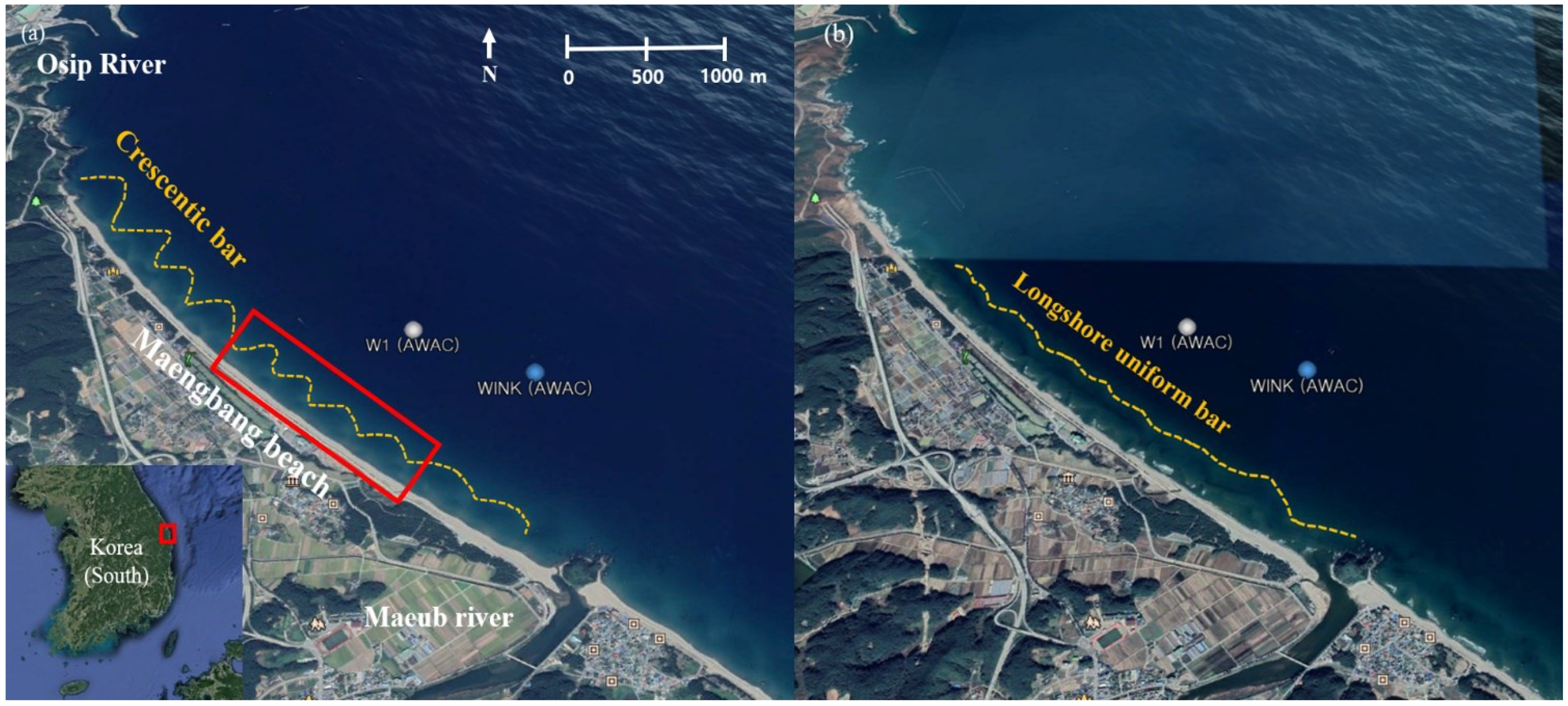
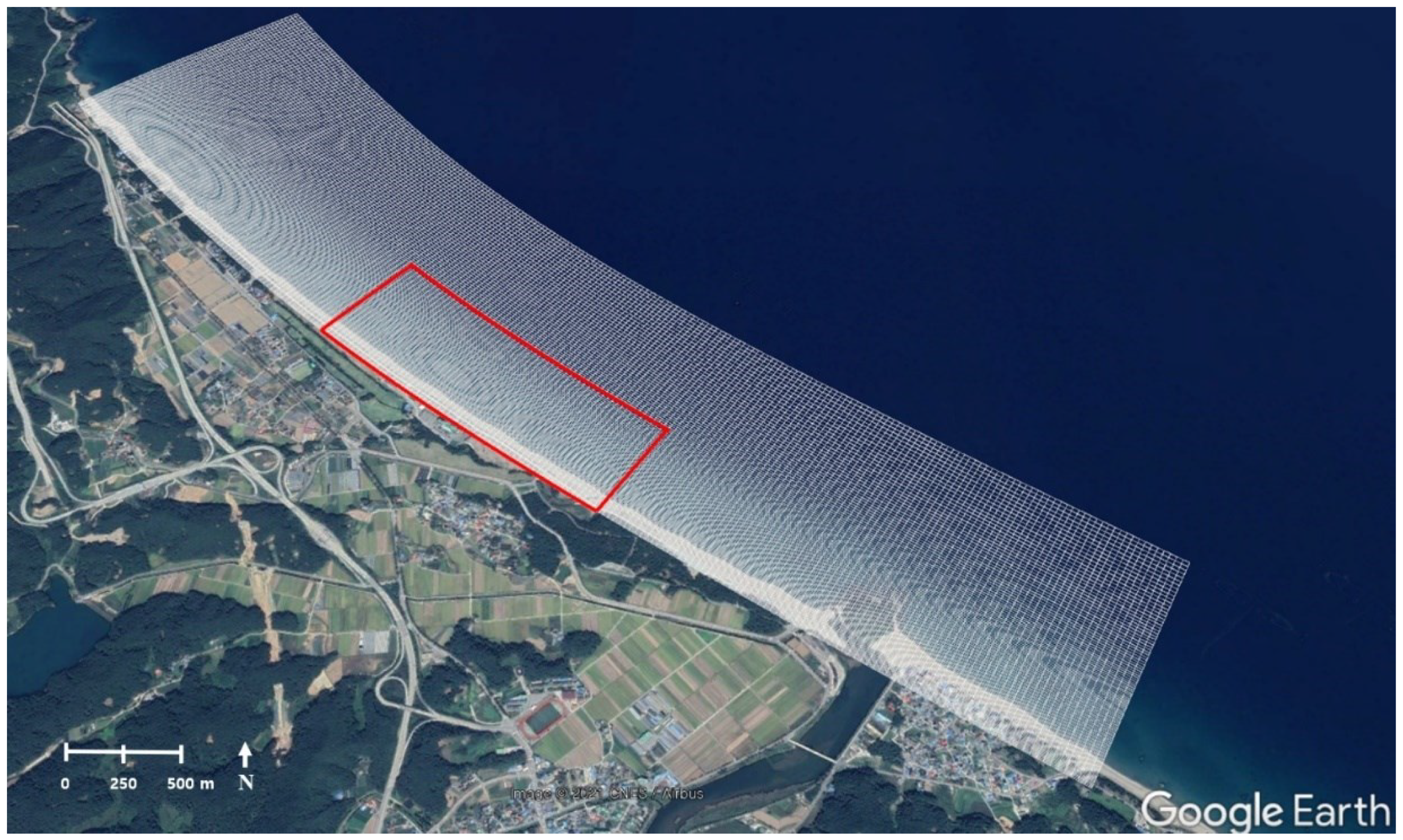
2.1. Study Area
2.2. Storm Events
2.2.1. S1
2.2.2. S2
2.2.3. C1
2.2.4. C2
3. Methodology
3.1. Numerical Setup
3.2. Model Calibration
3.3. Assessment of Event-Specific Calibration Data
4. Results
4.1. Influence of Event-Specific Datasets on Model Calibration
4.2. Parameter Sensitivity
4.3. Predicition of Profile Changes after Storm Events with an Optimum Parameter Set
5. Discussions and Conclusions
- The cumulative storm power and resultant erosion volume closely correlated with the overall model sensitivity compared to other features in the datasets (e.g., wave directions, pre-storm beach state, and the time interval between bathymetric surveys) at the study site. This result may help modelers decide which factors preferentially have to be considered in calibration in the area model under complex bathymetry.
- The analysis of model sensitivity to different storm events guides the selection of event-specific data for model calibration.
- XBSB can simulate the equilibrium profile response with reduced uncertainty and equifinality induced by the trial of various parameter combinations.
- This study highlights the effect of event-specific calibration of a process-based model in realizing better prediction and forecasting of coastal erosion, thereby resulting in more effective hazard mitigation. Therefore, the results of this study will benefit not only researchers but also government agencies involved in disaster management.
Author Contributions
Funding
Institutional Review Board Statement:
Informed Consent Statement:
Data Availability Statement
Conflicts of Interest
References
- Vousdoukas, M.I.; Ranasinghe, R.; Mentaschi, L.; Plomaritis, T.A.; Athanasiou, P.; Luijendijk, A.; Feyen, L. Sandy coastlines under threat of erosion. Nat. Clim. Chang. 2020, 10, 260–263. [Google Scholar] [CrossRef]
- Matheen, N.; Harley, M.D.; Turner, I.L.; Splinter, K.D.; Thran, M.C.; Simmons, J.A. Bathymetric Data Requirements for Operational Coastal Erosion Forecasting Using XBeach. J. Mar. Sci. Eng. 2021, 9, 1053. [Google Scholar] [CrossRef]
- Kobayashi, N.; Farhadzadeh, A.; Melby, J.; Johnson, B.; Gravens, M. Wave overtopping of levees and overwash of dunes. J. Coast. Res. 2010, 2010, 888–900. [Google Scholar] [CrossRef]
- Larson, M.; Kraus, N.C. SBEACH: Numerical Model for Simulating Storm-Induced Beach Change; Report 1, Empirical Foundation and Model Development ; Technical Report CERC-89-9; U.S Army Engineer Waterways Experiment Station, Coastal Engineering Research Center: Washington, DC, USA, 1989. [Google Scholar]
- Roelvink, D.; Reniers, A.; van Dongeren, A.; van Thiel de Vries, J.; McCall, R.; Lescinski, J. Modelling storm impacts on beaches, dunes and barrier islands. Coast. Eng. 2009, 56, 1133–1152. [Google Scholar] [CrossRef]
- Simmons, J.A.; Harley, M.D.; Marshall, L.A.; Turner, I.L.; Splinter, K.D.; Cox, R.J. Calibrating and assessing uncertainty in coastal numerical models. Coast. Eng. 2017, 125, 28–41. [Google Scholar] [CrossRef]
- Simmons, J.A.; Splinter, K.D.; Harley, M.D.; Turner, I.L. Calibration data requirements for modelling subaerial beach storm erosion. Coast. Eng. 2019, 152, 103507. [Google Scholar] [CrossRef]
- Elsayed, S.M.; Oumeraci, H. Effect of beach slope and grain-stabilization on coastal sediment transport: An attempt to overcome the erosion overestimation by XBeach. Coast. Eng. 2017, 121, 179–196. [Google Scholar] [CrossRef]
- Van Enckevort, I.M.J.; Ruessink, B.G.; Coco, G.; Suzuki, K.; Turner, I.L.; Plant, N.G.; Holman, R.A. Observations of nearshore crescentic sandbars. J. Geophys. Res. Ocean. 2004, 109, 1–17. [Google Scholar] [CrossRef]
- Castelle, B.; Ruessink, B.G.; Bonneton, P.; Marieu, V.; Bruneau, N.; Price, T.D. Coupling mechanisms in double sandbar systems. Part 1: Patterns and physical explanation. Earth Surf. Process. Landf. 2010, 35, 476–486. [Google Scholar] [CrossRef]
- Orzech, M.D.; Reniers, A.J.H.M.; Thornton, E.B.; MacMahan, J.H. Megacusps on rip channel bathymetry: Observations and modeling. Coast. Eng. 2011, 58, 890–907. [Google Scholar] [CrossRef]
- Price, T.D.; Ruessink, B.G.; Castelle, B. Morphological coupling in multiple sandbar systems—A review. Earth Surf. Dyn. 2014, 2, 309–321. [Google Scholar] [CrossRef]
- Ranasinghe, R.; Turner, I.L. Shoreline response to submerged structures: A review. Coast. Eng. 2006, 53, 65–79. [Google Scholar] [CrossRef]
- Nordstrom, K.F. Living with shore protection structures: A review. Estuar. Coast. Shelf Sci. 2014, 150, 11–23. [Google Scholar] [CrossRef]
- Bolle, A.; Mercelis, P.; Roelvink, D.; Haerens, P.; Trouw, K. Application and Validation of Xbeach for Three Different Field Sites. Coast. Eng. Proc. 2011, 1, 40. [Google Scholar] [CrossRef]
- Simmons, J.A. Improved Model Calibration Techniques for Predicting Coastal Storm Erosion. Ph.D. Thesis, The University of New South Wales, Sydney, Australia, March 2018. [Google Scholar]
- Pender, D.; Karunarathna, H. A statistical-process based approach for modelling beach profile variability. Coast. Eng. 2013, 81, 19–29. [Google Scholar] [CrossRef]
- Kalligeris, N.; Smit, P.; Ludka, B.C.; Guza, R.T.; Gallien, T.W. Calibration and assessment of process-based numerical models for beach profile evolution in southern California. Coast. Eng. 2020, 158, 103650. [Google Scholar] [CrossRef]
- Kombiadou, K.; Costas, S.; Roelvink, D. Simulating destructive and constructive morphodynamic processes in steep beaches. J. Mar. Sci. Eng. 2021, 9, 86. [Google Scholar] [CrossRef]
- Rafati, Y.; Hsu, T.J.; Elgar, S.; Raubenheimer, B.; Quataert, E.; van Dongeren, A. Modeling the hydrodynamics and morphodynamics of sandbar migration events. Coast. Eng. 2021, 166, 103885. [Google Scholar] [CrossRef]
- Karunarathna, H.; Pender, D.; Ranasinghe, R.; Short, A.D.; Reeve, D.E. The effects of storm clustering on beach profile variability. Mar. Geol. 2014, 348, 103–112. [Google Scholar] [CrossRef]
- Dissanayake, P.; Brown, J.; Wisse, P.; Karunarathna, H. Effects of storm clustering on beach/dune evolution. Mar. Geol. 2015, 370, 63–75. [Google Scholar] [CrossRef]
- Callaghan, D.P.; Ranasinghe, R.; Roelvink, D. Probabilistic estimation of storm erosion using analytical, semi-empirical, and process based storm erosion models. Coast. Eng. 2013, 82, 64–75. [Google Scholar] [CrossRef]
- De Boer, W.; Huisman, B.; Yoo, J.; McCall, R.; Scheel, F.; Swinkels, C.M.; Friedman, J.; Luijendijk, A.; Walstra, D. Understanding coastal erosion processes at the Korean east coast. In Proceedings of the Coastal Dynamics 2017, Helsingør, Denmark, 12–16 June 2017; pp. 1336–1347. Available online: https://pure.tudelft.nl/ws/files/31196730/014_DeBoer_Wiebe.pdf (accessed on 11 August 2022).
- Jin, H.; Do, K.; Chang, S.; Kim, I.H. Field Observation of Morphological Response to Storm Waves and Sensitivity Analysis of XBeach Model at Beach and Crescentic Bar. J. Korean Soc. Coast. Ocean Eng. 2020, 32, 446–457. [Google Scholar] [CrossRef]
- Van Rijn, L.C.; Wasltra, D.J.R.; Grasmeijer, B.; Sutherland, J.; Pan, S.; Sierra, J.P. The predictability of cross-shore bed evolution of sandy beaches at the time scale of storms and seasons using process-based profile models. Coast. Eng. 2003, 47, 295–327. [Google Scholar] [CrossRef]
- Wright, L.D.; Short, A.D. Morphodynamic variability of surf zones and beaches: A synthesis. Mar. Geol. 1984, 56, 93–118. [Google Scholar] [CrossRef]
- Cho, Y.J.; Kim, I.H. Preliminary Study on the Development of a Platform for the Selection of Optimal Beach Stabilization Measures against the Beach Erosion—Centering on the Yearly Sediment Budget of Mang-Bang Beach. J. Korean Soc. Coast. Ocean Eng. 2019, 31, 28–39. [Google Scholar] [CrossRef]
- Oh, S.-H.; Jeong, W.-M.; Lee, D.-Y.; Kim, S. Analysis of the Reason for Occurrence of Large- Height Swell-like Waves in the East Coast of Korea Analysis of the Reason for Occurrence of Large-Height Swell-like Waves in the East Coast of Korea. J. Korean Soc. Coast. Ocean Eng. 2010, 22, 101–111. [Google Scholar]
- Castelle, B.; Marieu, V.; Bujan, S.; Splinter, K.D.; Robinet, A.; Sénéchal, N.; Ferreira, S. Impact of the winter 2013-2014 series of severe Western Europe storms on a double-barred sandy coast: Beach and dune erosion and megacusp embayments. Geomorphology 2015, 238, 135–148. [Google Scholar] [CrossRef]
- Dissanayake, P.; Brown, J.; Karunarathna, H. Impacts of storm chronology on the morphological changes of the Formby beach and dune system, UK. Nat. Hazards Earth Syst. Sci. 2015, 15, 1533–1543. [Google Scholar] [CrossRef]
- Wright, L.D.; Short, A.D.; Green, M.O. Short-term changes in the morphodynamic states of beaches and surf zones: An empirical predictive model. Mar. Geol. 1985, 62, 339–364. [Google Scholar] [CrossRef]
- Yates, M.L.; Guza, R.T.; O’Reilly, W.C.; Hansen, J.E.; Barnard, P.L. Equilibrium shoreline response of a high wave energy beach. J. Geophys. Res. Ocean. 2011, 116, 1–13. [Google Scholar] [CrossRef]
- Ludka, B.C.; Guza, R.T.; O’Reilly, W.C.; Yates, M.L. Field evidence of beach profile evolution toward equilibrium. J. Geophys. Res. Ocean. 2015, 120, 7574–7597. [Google Scholar] [CrossRef] [Green Version]
- Athanasiou, P. Understanding the Interactions between Crescentic Bars, Human Interventions and Coastline Dynamics at the East Coast of South Korea. Master’s Thesis, Delft University of Technologyt, Delft, The Netherlands, 19 September 2017. [Google Scholar]
- Cohn, N.; Ruggiero, P.; Ortiz, J.; Walstra, D.J. Investigating the role of complex sandbar morphology on nearshore hydrodynamics. J. Coast. Res. 2014, 70, 53–58. [Google Scholar] [CrossRef]
- Do, K.; Yoo, J. Morphological response to storms in an embayed beach having limited sediment thickness. Estuar. Coast. Shelf Sci. 2020, 234, 106636. [Google Scholar] [CrossRef]
- Passeri, D.L.; Long, J.W.; Plant, N.G.; Bilskie, M.V.; Hagen, S.C. The influence of bed friction variability due to land cover on storm-driven barrier island morphodynamics. Coast. Eng. 2018, 132, 82–94. [Google Scholar] [CrossRef]
- Roelvink, D.; Costas, S. Beach berms as an essential link between subaqueous and subaerial beach/dune profiles. Geo-Temas 2017, 17, 79–82. [Google Scholar]
- Van der Lugt, M.A.; Quataert, E.; van Dongeren, A.; van Ormondt, M.; Sherwood, C.R. Morphodynamic modeling of the response of two barrier islands to Atlantic hurricane forcing. Estuar. Coast. Shelf Sci. 2019, 229, 106404. [Google Scholar] [CrossRef]
- Fang, K.; Wang, H.; Sun, J.; Zhang, J.; Liu, Z. Including Wave Diffraction in XBeach: Model Extension and Validation. J. Coast. Res. 2020, 36, 116. [Google Scholar] [CrossRef]
- Daly, C.; Roelvink, D.; van Dongeren, A.; van Thiel de Vries, J.; McCall, R. Validation of an advective-deterministic approach to short wave breaking in a surf-beat model. Coast. Eng. 2012, 60, 69–83. [Google Scholar] [CrossRef]
- Cho, M.; Yoon, H.D.; Do, K.; Kim, I. Calibration and Assessment of Bed Evolution Model in an Embayed Beach with Submerged Breakwaters. J. Coast. Res. 2021, 114, 514–518. [Google Scholar] [CrossRef]
- Nederhoff, C.M. (Kees) Modelling the Effects of Hard Structures on Dune Erosion and Overwash. Hindcasting the Impact of Hurricane Sandy on New Jersey with XBeach. Master’s Thesis, Delft University of Technology, Delft, The Netherlands, 14 November 2014. [Google Scholar]
- De Vet, P.L.M.; McCall, R.T.; Den Bien, J.P.; Stive, M.J.F.; Van Ormondt, M. Modelling Dune Erosion, Overwash and Breaching at Fire Island (Ny) during Hurricane Sandy. In Proceedings of the Coastal Sediment 2015, San Diego, CA, USA, 11–15 May 2015; pp. 1–10. [Google Scholar]
- Roelvink, J.A. Dissipation in random wave groups incident on a beach. Coast. Eng. 1993, 19, 127–150. [Google Scholar] [CrossRef]
- Daly, C.; Roelvink, D.; Van Dongeren, A.; Van Thiel de Vries, J.; McCall, R. Short Wave Breaking Effects on Low Frequency Waves. Coast. Eng. Proc. 2011, 1, 20. [Google Scholar] [CrossRef]
- Roelvink, D.; McCall, R.; Mehvar, S.; Nederhoff, K.; Dastgheib, A. Improving predictions of swash dynamics in XBeach: The role of groupiness and incident-band runup. Coast. Eng. 2018, 134, 103–123. [Google Scholar] [CrossRef]
- Van Thiel de Vries, J. Dune erosion above revetments. In Proceedings of the 33rd International Conference on Coastal Engineering, Santander, Spain, 1–6 July 2012; pp. 1–13. [Google Scholar]
- Bae, H.; Do, K.; Kim, I.H.; Chang, S. Proposal of parameter range that offered optimal performance in the coastal morphodynamic model (XBeach) through GLUE. J. Ocean Eng. Technol. 2022, 36, 251–269. [Google Scholar] [CrossRef]
- Soulsby, R.L. Dynamics of Marine Sands; Thomas Telford Publications: London, UK, 1997. [Google Scholar]
- Hornberger, G.M.; Spear, R.C. An approach to the preliminary analysis of environmental systems. J. Environ. Manag. 1981, 12, 7–18. [Google Scholar]
- Daly, C.; Floc’h, F.; Almeida, L.P.; Almar, R. Modelling accretion at nha trang beach, vietnam. In Proceedings of the International Conference on Coastal Dynamics, Helsingor, Denmark, 12–16 June 2017; pp. 1886–1896. [Google Scholar]
- Stockdon, H.F.; Thompson, D.M.; Plant, N.G.; Long, J.W. Evaluation of wave runup predictions from numerical and parametric models. Coast. Eng. 2014, 92, 1–11. [Google Scholar] [CrossRef]
- Palmsten, M.L.; Splinter, K.D. Observations and simulations of wave runup during a laboratory dune erosion experiment. Coast. Eng. 2016, 115, 58–66. [Google Scholar] [CrossRef]
- De Beer, A.F.; McCall, R.T.; Long, J.W.; Tissier, M.F.S.; Reniers, A.J.H.M. Simulating wave runup on an intermediate–reflective beach using a wave-resolving and a wave-averaged version of XBeach. Coast. Eng. 2021, 163, 103788. [Google Scholar] [CrossRef]


| Storm Event | Time Interval between Bathymetric Survey (Days) | Pre-Storm Survey (Days before Initial Storm Starts) | Post-Storm Survey (Days after Final Storm Ends) | Number of Storms | Each Storm Duration (Hours) | Each Storm Power | Characteristics at Each Storm Peak Hs | ||||
|---|---|---|---|---|---|---|---|---|---|---|---|
| Cumulative Storm Power m2h | Hs (m) | Tp (s) | Dp (deg. N) | Water Level (m) | |||||||
| S1 | 2017-09-08~10/26 (48) | 44.6 | 1.8 | 1 | 38 | 490 | 490 | 4.5 | 10.2 | 57.1 | −0.25 |
| S2 | 2020-05-07~05/28 (21) | 11.7 | 6.8 | 1 | 59 | 506 | 506 | 4.2 | 11.5 | 47.6 | 0.19 |
| C1 | 2019-08-29~10/30 (62) | 24.6 | 14.8 | 5 | 39 27 18 32 10 | 508 218 167 363 94 | 1350 | 4.5 3.2 3.8 4.2 3.5 | 10.9 10.1 10.7 10.5 9.3 | 69.1 40.5 42.1 53.4 42.5 | −0.03 0.34 0.17 −0.12 0.01 |
| C2 | 2020-08-20~09/18 (29) | 14.2 | 3.5 | 3 | 5 12 42 | 60 129 478 | 667 | 3.9 4.4 4.7 | 9.3 10.4 11.4 | 87.8 63.0 46.2 | 0.83 0.39 0.06 |
| Parameter | Description | Values |
|---|---|---|
| facua * | Adjustable parameters for parameterizing both wave skewness (facSk) and asymmetry (facAs) | 0.10, 0.15, 0.20, 0.25 |
| alpha * | Wave dissipation coefficient for short wave breaking | 1, 2 |
| gamma * | Breaker parameter in RvDaly formulation, with larger values of gamma encouraging less wave dissipation (See [44] for details) | 0.42, 0.52, 0.62 |
| gamma2 * | Reformation parameter in RvDaly formulation, with larger values of gamma2 encouraging less wave dissipation (See [44] for details) | 0.25, 0.30, 0.35, 0.40 |
| D50 | D50 sediment diameter applied to the model domain | 0.4 mm |
| D90 | D90 sediment diameter applied to the model domain | 0.7 mm |
| bedfriccoef | Bed friction coefficient defined as Chezy value, influencing mean flows and long waves | /s |
| break | Type of breaker formulation | roelvink_daly [42] |
| form | Type of sediment transport formulation | soulsby_vanrijn [51] |
| Storm Events | S2 | S1 | C2 | C1 |
|---|---|---|---|---|
| Number of storms | 1 | 1 | 3 | 5 |
| K–S D | 0.14 | 0.23 | 0.29 | 0.45 |
| Cumulative storm power (m2h) | 506 | 490 | 667 | 1350 |
| Maximum Hs (m) | 4.2 | 4.5 | 4.7 | 4.5 |
| 30.4 | 31.3 | 43.9 | 48.2 | |
| (deg. N) | 47.6 | 57.1 | 87.8, 63.0, 46.2 | 69.1, 40.5, 42.1, 53.4, 42.5 |
| Interval between bathymetric survey (Days) | 21 | 48 | 29 | 62 |
Publisher’s Note: MDPI stays neutral with regard to jurisdictional claims in published maps and institutional affiliations. |
© 2022 by the authors. Licensee MDPI, Basel, Switzerland. This article is an open access article distributed under the terms and conditions of the Creative Commons Attribution (CC BY) license (https://creativecommons.org/licenses/by/4.0/).
Share and Cite
Jin, H.; Do, K.; Kim, I.; Chang, S. Sensitivity Analysis of Event-Specific Calibration Data and Its Application to Modeling of Subaerial Storm Erosion under Complex Bathymetry. J. Mar. Sci. Eng. 2022, 10, 1389. https://doi.org/10.3390/jmse10101389
Jin H, Do K, Kim I, Chang S. Sensitivity Analysis of Event-Specific Calibration Data and Its Application to Modeling of Subaerial Storm Erosion under Complex Bathymetry. Journal of Marine Science and Engineering. 2022; 10(10):1389. https://doi.org/10.3390/jmse10101389
Chicago/Turabian StyleJin, Hyeok, Kideok Do, Inho Kim, and Sungyeol Chang. 2022. "Sensitivity Analysis of Event-Specific Calibration Data and Its Application to Modeling of Subaerial Storm Erosion under Complex Bathymetry" Journal of Marine Science and Engineering 10, no. 10: 1389. https://doi.org/10.3390/jmse10101389
APA StyleJin, H., Do, K., Kim, I., & Chang, S. (2022). Sensitivity Analysis of Event-Specific Calibration Data and Its Application to Modeling of Subaerial Storm Erosion under Complex Bathymetry. Journal of Marine Science and Engineering, 10(10), 1389. https://doi.org/10.3390/jmse10101389