Article

Predicting the Sound Speed of Seafloor Sediments in the East China Sea Based on an XGBoost Algorithm

1
Key Laboratory of Marine Geology and Metallogeny, First Institute of Oceanography, Ministry of Natural Resources, Qingdao 266061, China
2
Laboratory for Marine Geology, Pilot National Laboratory for Marine Science and Technology (Qingdao), Qingdao 266237, China
3
College of Underwater Acoustic Engineering, Harbin Engineering University (Harbin), Harbin 150001, China
*
Author to whom correspondence should be addressed.
J. Mar. Sci. Eng. 2022, 10(10), 1366; https://doi.org/10.3390/jmse10101366
Submission received: 7 August 2022 / Revised: 18 September 2022 / Accepted: 19 September 2022 / Published: 24 September 2022
(This article belongs to the Special Issue Advances in Marine Engineering: Geological Environment and Hazards)

Abstract

:
Based on the acoustic and physical data of typical seafloor sediment samples collected in the East China Sea, this study on the super parameter selection and contribution of the characteristic factors of the machine learning model for predicting the sound speed of seafloor sediments was conducted using the eXtreme gradient boosting (XGBoost) algorithm. An XGBoost model for predicting the sound speed of seafloor sediments was established based on five physical parameters: density ( ρ ), water content ( w ), void ratio ( e ), sand content (S), and average grain size (Mz). The results demonstrated that the model had the highest accuracy when n_estimator was 75 and max_depth was 5. The model training goodness of fit (R2) was as high as 0.92, and the mean absolute error and mean absolute percent error of the model prediction were 7.99 m/s and 0.51%, respectively. The results demonstrated that, in the study area, the XGBoost prediction method for the sound speed of seafloor sediments was superior to the traditional single- and two-parameter regressional equation prediction methods, with higher prediction accuracy, thus providing a new approach to predict the sound speed of seafloor sediments.

1. Introduction

The shallow sediments of the seafloor exhibit unique acoustic properties that provide the necessary basic data for seafloor acoustic field research, seafloor engineering geology, and marine petroleum geology and are important factors in determining the marine acoustic field environment [1]. They have important research value in the fields of seafloor sediment investigation, marine resource exploration and development, and marine environmental monitoring [2,3]. Seafloor sediments are generally considered a two-phase medium consisting of solid and liquid phases [4], and their acoustic properties are closely related to the physical properties of seafloor sediments.
As the basic element of seafloor acoustics research, the measuring methods of the sound speed of seafloor sediments primarily include in situ measurements, laboratory measurements, and the geoacoustic inversion method. In addition, prediction based on geoacoustic models is an important method for obtaining the sound speed of seafloor sediments. Therefore, it is extremely important to establish an accurate geoacoustic model to describe the relationship between the sediment sound speed and physical parameters. Many studies established theoretical models for predicting sound speed in seafloor sediments [5,6,7,8,9,10,11]. However, because of the complex and diverse marine sedimentary environment and sedimentary disturbance error in the determination process, the several input parameters of the theoretical model are difficult to measure. Concomitantly, many studies have established regressional equations of sound speed prediction in different sea areas by examining the correlation between the sound speed and physical parameters of seafloor sediments [12,13,14,15,16,17,18,19,20,21,22]. However, the physical properties of sediments frequently require multiple parameters for accurate characterization. The empirical equation only establishes the correlation between the sediment sound speed and one or two physical parameters to an extent, and there are limitations and reduced accuracy in the sound speed prediction.
To supplement the existing literature, this study proposes a machine learning prediction method for the sound speed of seafloor sediments based on the eXtreme gradient boosting (XGBoost) algorithm, which can fuse multiple sediment physical parameters as well as effectively improve the problem of the previous empirical equations tending to overfit or underfit the measured sound speed of seafloor sediment Here, data preprocessing was performed on the data measured at laboratory of sediment samples from the East China Sea. The physical parameters with high correlation were then extracted using the Pearson correlation coefficient matrix, and the model was trained and verified. Then, using the test samples and traditional single- and two-parameter regressional equations to comprehensively evaluate the model, we analyzed the contribution of each physical parameter. The results demonstrated that the prediction model of the seafloor sediment sound speed based on the XGBoost algorithm was superior to the traditional prediction equation methods with higher prediction accuracy.

2. Study Area and Data Source

2.1. Location of the Study Area

The study area is located on the continental shelf of the East China Sea at a water depth of 26–107 m. The water depth of the western-inland region is shallow and gradually increases to the east. As one of the widest continental shelves worldwide, it has considerable terrigenous input and is an important area for studying land–ocean interactions and source–sink processes [23]. The deposition of terrigenous sediments in this area is primarily controlled by the coastal upwelling and downwelling of the southern continental shelf of the East China Sea [24]. Owing to the inflow of small coastal rivers such as the Yangtze River and the influence of the Yellow River, the continental shelf of the East China Sea has received a high input of terrigenous materials [25]. In the interaction between the Zhejiang–Fujian coastal current and Taiwan warm current, most sediments diffused from the north to the south were confined in the continental shelf, thus forming an intrashelf mud wedge [26]; however, most of the sediments in the study area were confined in the continental shelf and covered by sand [27]. The coastal sediments in the study area are parallel to the coast and distributed in a band, and the nearshore is mostly silty clay, whereas the outward is clay. The sediment then quickly changes to coarse-grained silt or fine sand.

2.2. Data Sources

Seafloor sediment samples were collected at 45 sites on the East China Sea shelf using box and gravity samplers during the open research cruise of the East China Sea supported by the National Science Foundation of China (NSFC) Shiptime Shearing Project in 2021. Among these samples, those that were ~400 cm in length were obtained from 16 stations in the East China Sea’s silty clay and clayey silt areas, while most obtained from the sandy bottom in the study area were 20–200 cm in length. The sound speed and physical parameters were measured in the laboratory. First, the sample was cut and divided as per the actual requirements, generally cut into 30 cm long sections and placed on a cylindrical sample measurement platform. The laboratory measurement system of the acoustic property of seafloor sediment cores was used to measure the sound speed of the sediment samples using the transmission method. After the 30 cm long sediment measurement was completed, a length of 10 cm was cut off, and the sound speed of the remaining 20 cm long sediment was measured again to obtain as much data as possible. The sound speed was calculated as follows:
V P = L / ( 10 3 ( t t 0 ) )
where V P is the sound speed of the seafloor sediment sample (m/s), L is the column length of the sample (mm), t is the sound wave penetration time (μs), and t0 is the correction value of zero sound time (μs).
After measuring the sound speed of the sample, the physical and mechanical properties of the sediment were measured [28]. The properties included density, water content, void ratio, sand content, silt content, clay content, and average grain size. During the laboratory measurements, two-frequency (25 and 100 kHz) acoustic transducers were used to measure the acoustic properties and physical parameters of each section of the sample. Because the acoustic data with a frequency of 100 kHz were of good quality and the covered physical parameters were more representative, although the sound speed values at different frequencies differed, the relationship between them and the physical properties of the sediments was the same. Thus, this study selected sound speed data of 100 kHz (292 groups). Table 1 lists the maximum, minimum, and average of the physical parameters and sound speeds.

3. Methods

3.1. Data Preprocessing

3.1.1. Data Noise Removal

The experimental data were collected from a real scene and contained a lot of data noise; therefore, they could not be directly used for model training. The primary task of data noise removal is to remove incomplete or wrong data. Here, data cleaning was divided into outlier and missing value removal. Data points significantly far from the fitted curve are marked as outliers using a regression fit between the sound speed and each physical parameter. The missing sound speed values and physical parameters of each sample were simultaneously removed to improve the data quality and integrity.

3.1.2. Normalization Processing

The numerical units of different physical parameters differ; therefore, the data required normalization. The parameters were uniformly set to a value between 0 and 1. Normalizing the input data can prevent neuron saturation and increase the accuracy and generalization ability of the model prediction. The formula of normalization is as follows:
X ¯ = X X min X max X min
where X ¯ is the normalized data, X is the original data, and X min and X max are the maximum and minimum values of the original data, respectively.

3.1.3. Physical Parameter Extraction

In order to reduce the complexity of the model and improve the generalization ability of the model, some but not all parameters with relatively strong correlation were selected while ensuring accuracy during the data processing. Here, the data collected included the sound speed, basic information of the following sampling stations, and physical parameters of the sediments:
  • Geospatial information of the seafloor sediment sampling stations—longitude (Log), latitude (Lat), and depth (D);
  • Basic physical parameters—density ( ρ ), water content ( w ), and void ratio ( e );
  • Grain composition—sand (S), silt (T), clay contents (Y);
  • Grain size coefficient—average grain size (Mz).
Among the acoustic parameters and physical and mechanical parameters of seafloor sediments, the sound speed exhibits a good correlation with the density, water content, and porosity [18]. The Pearson correlation coefficient can measure the degree of correlation and whether there is a linear correlation between two features [29]. Thus, the Pearson correlation coefficient was used to measure the correlation between the sound speed and other physical parameters and plot the correlation coefficient matrix (Figure 1). Using two variables—X and Y—the Pearson correlation coefficient between the variables is as follows:
f X , Y = E ( XY ) E ( X ) E ( Y ) E ( X 2 ) + E 2 ( X ) E ( Y 2 ) + E 2 ( Y )
where f X , Y is the correlation coefficient. A positive value indicates a positive correlation between the physical parameters and sound speed, and a negative value indicates a negative correlation.
As per the first column of the matrix diagram of the correlation coefficient between the sound speed and each physical parameter (Figure 1), it was concluded that the correlation coefficient between the sound speed and density, water content, void ratio, sand content, and average particle size of the seafloor sediments reached ~0.90, exhibiting strong or extremely strong correlation. The correlation coefficient with other parameters was below 0.80. During the training of the XGBoost algorithm model, the highest correlation between the input feature factor and target parameter was selected such that the predicted result was closer to the expected value. Similarly, the dimension of the model was reduced as much as possible while ensuring the accuracy of the model to reduce the complexity of the model. Therefore, the factors selected for training in this study were the density, water content, void ratio, sand content, and average grain size. Among these factors, the density and sand content positively correlated with the sound speed, indicating that the higher the density and sand content, the higher the sound speed. The water content, void ratio, and average grain size negatively correlated with the sound speed, indicating that with an increase in each parameter, the sound speed decreased.

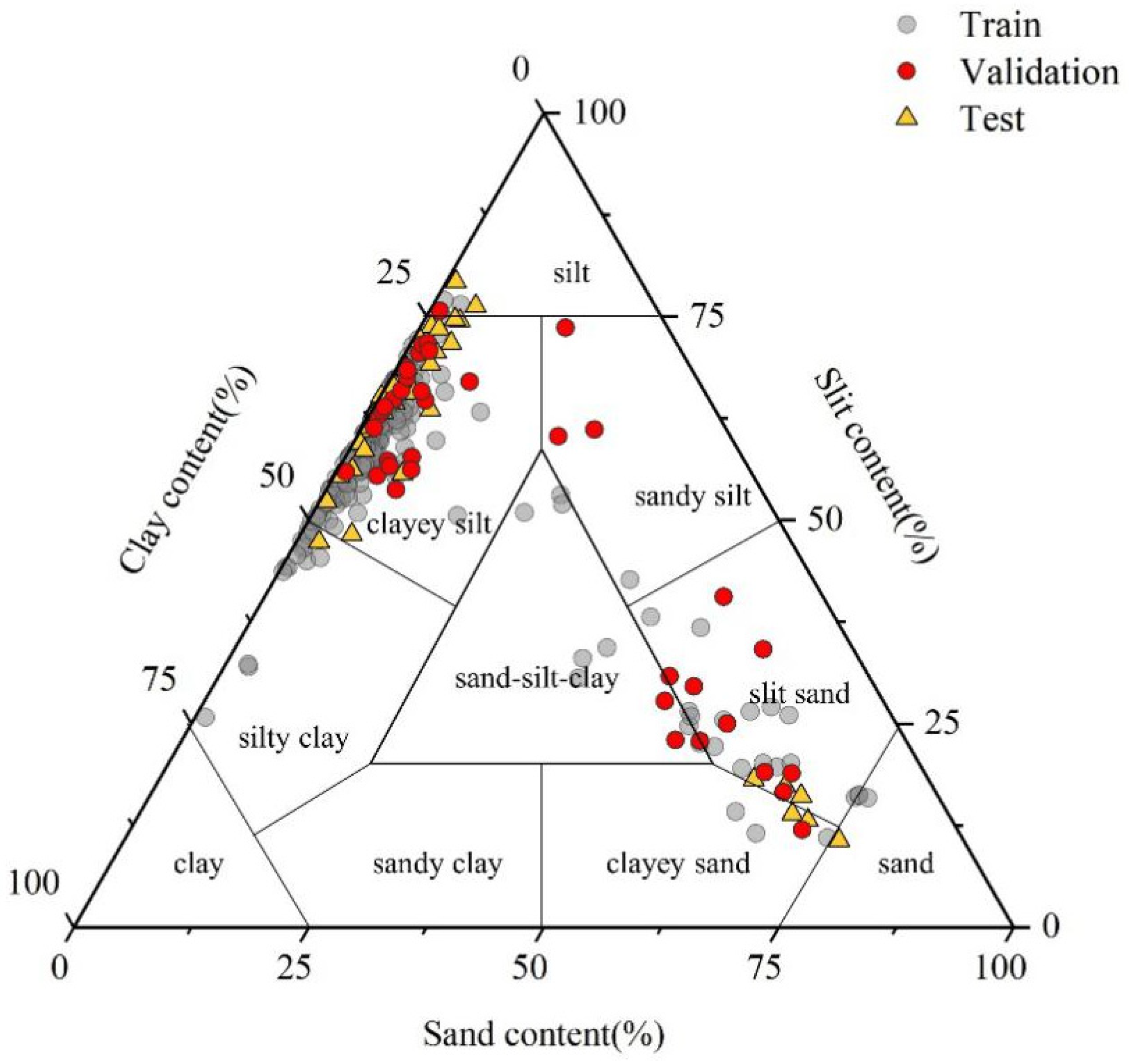
3.1.4. Data Division

After data preprocessing, 280 data sample groups were collected, and the samples were randomly divided into 200 training, 40 validation, and 40 test sample groups. After the training, validation, and test sets were determined, only then were the parameters of the learning algorithm adjusted to explore suitable parameters, screen suitable features, rapidly detect the algorithm performance, and guide the most important changes to the machine learning model. The training samples were used to train the sound speed prediction model, and the final model was trained by setting the parameters of the fitter. After training multiple models via the training set, the model with the best effect was selected from the validation set. The corresponding parameters can then be used to control the occurrence of model over-fitting. To measure the performance of the optimized model, the test samples were considered as a nonexistent data set—a data sample that did not participate in the entire model building process and was used to measure the performance of the optimized model. Figure 2 shows the training, validation, and test samples in the sediment triangulation. There were multiple types of sediments in the data samples, which improved the generalization ability of the model.

3.2. XGBoost Algorithm

XGBoost is a boosted tree model that integrates multiple weak learners to build a strong learner [30,31]. The idea of the algorithm is to fit the negative gradient of the loss function in repeated iterations after optimizing the empirical loss function, select sample features to generate a basic learner, and continuously fit the previous residuals to minimize the objective function. We repeated this process to build hundreds of basic learners and integrated them in a comprehensive model (Figure 3).
The objective function of XGBoost comprises a loss function, regularization term, and constant term. The equation is as follows:
Obj ( θ ) = L ( θ ) + Ω ( θ ) + C
The loss function was used to measure the quality of the model prediction, and the regularization term was used to control the complexity of the model and avoid overfitting.

3.2.1. Loss Function

The XGBoost algorithm can be considered as an additive model comprising K trees, as shown in Equation (5). The tree model used in this study is a regression tree:
y ^ i = k = 1 K f k ( x i ) , f k F
where y ^ i is the sample prediction result, x i , i is the i-th sample input, k is the sum of trees, f k is each regression tree, and F is the set space with the regression tree.
The improvement of XGBoost over the Gradient Boosting Decision Tree (GBDT) is that it uses the first- and second-order derivatives and the Taylor expansion for approximation. If g i is the first derivative and h i is the second derivative:
g i = y ^ ( t 1 ) l ( y i , y ^ i ( t 1 ) )
h i = y ^ ( t 1 ) 2 l ( y i , y ^ i ( t 1 ) )

3.2.2. Regularization

The complexity of the regression tree can effectively control the overfitting of the model. It comprises two parts: the number and weight of leaf nodes. It was defined by the equation as:
Ω ( f t ) = γ T + 1 2 λ j = 1 T w j 2
where γ and λ are the normalization coefficients. Combining the two aforementioned parts, the objective function was rewritten as the following equation:
Obj ( θ ) j = 1 T [ ( i I j g i ) w j + 1 2 ( i I j h i + λ ) w j 2 ] + γ T
where I j is the sample on the j-th leaf node, and w j is the weight of the j-th leaf node. The optimal objective function was then obtained:
Obj ( θ ) = 1 2 j = 1 T G j H j + λ + γ T
The smaller the objective function, the smaller the prediction error, and the better the model effect.

4. Results

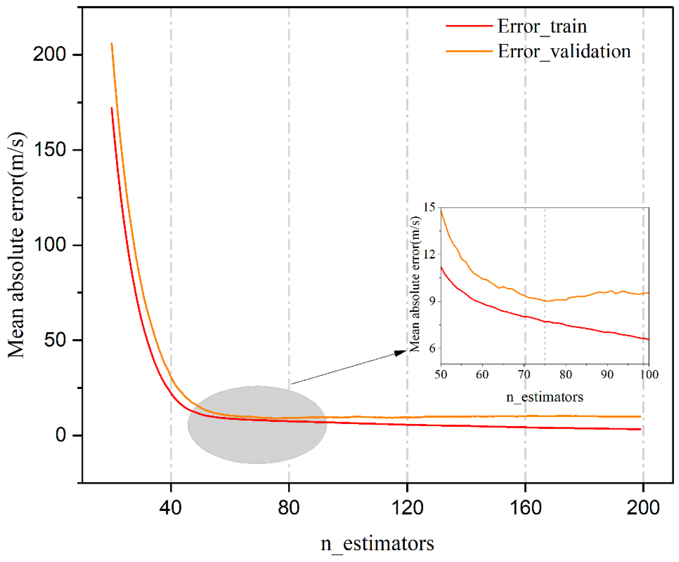
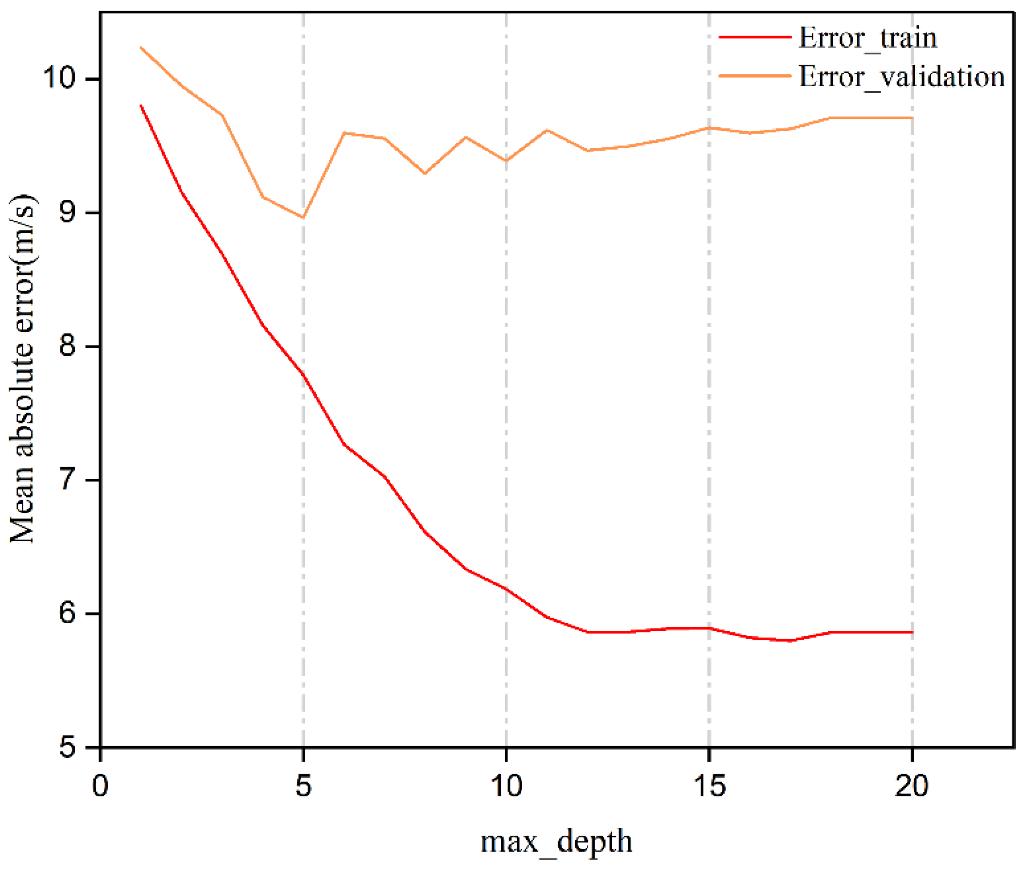
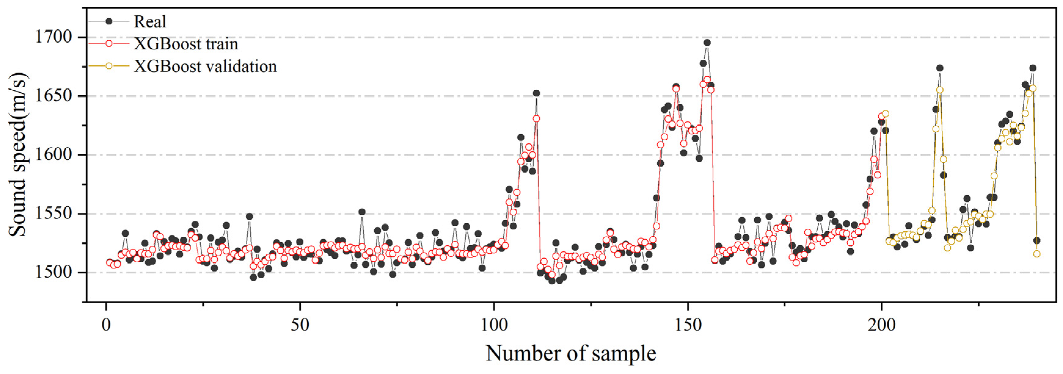
4.1. Training and Validation of Seafloor Sediment Prediction Model

This study was based on the XGBoost algorithm with the CART (Classification and Regression Tree) as the base learner. The 200 sets of training data obtained in the laboratory were used for model training, and the 40 sets of validation samples were used to assist the model training to obtain optimal parameters such that the model performance could reach the highest level. The selected training target parameter was the sediment sound speed; the characteristic factors were the density, water content, void ratio, average grain size, and clay content. During the model training process, the XGBoost algorithm had multiple hyperparameters, and it was impossible to adjust all the parameters. Therefore, this study optimized two parameters—n_estimator and max_depth, which were important to the model training accuracy—and the parameter adjustment and optimization followed the principle of “first importantly then weak, first coarse then fine.” Here, the mean absolute error (MAE) and mean absolute percentage error (MAPE) were selected to compare the performance of different models. The equations of the two indicators are as follows:
M A E = i = 1 n | y ^ i y i | n
M A P E = 100 % n i = 1 n | y ^ i y i y i |
where y i is the true value, y ^ i is the predicted value, and n is the number of predicted samples.
The n_estimator in the XGBoost hyperparameters, i.e., the maximum number of trees, can be considered as the number of iterations that determines the learning ability of the model. The greater the number of trees, the stronger the learning ability of the model. When the number of trees in the XGBoost was low, the impact on the model was relatively high; when the number of trees was already high, the impact on the model was relatively low. The smaller the trees, the easier it was to cause the model to under-fit, and excess trees easily caused the model to over-fit. Therefore, selecting the appropriate n_estimator can impact the training accuracy of the model. Here, the optimal selection of the n_estimator was made within the range of [20, 200]. As shown in Figure 4, when the n_estimator exceeded 75, the training error of the model continually decreased, and the error of the validation sample gradually increased. Therefore, it was determined that when the n_estimator exceeded 75, the model was in the overfitting state, and so the n_estimator of the research model was 75, and the model effect was the best. At this time, the goodness of fit (R2) of the model training was 0.917, the real value of the MAE of the training result was 8.15 m/s, and that of the validation result was 9.11 m/s.
The max_depth is the maximum depth of the tree in the model, which is used to control the model fitting state. The larger the max_depth, the more specific the model learns; however, if the max_depth is excessively large, the model overfits. Based on the premise that A in the model was 75, this study set the max_depth to perform optimal model training in [1,20]. As shown in Figure 5, when the max_depth was 5, the model had the highest validation accuracy. At this time, the R2 of the model training was 0.923, the real value of the MAE of the training result was 7.79 m/s, and that of the validation result was 8.96 m/s.
After the continuous optimization of the model, along with the error performance of the training and validation results, the optimal model had an n_estimator and max_depth of 75 and 5, respectively. Figure 6 shows that the training results of the 200 training sample groups and validation results of 40 validation sample groups had a high degree of fit with the real values.

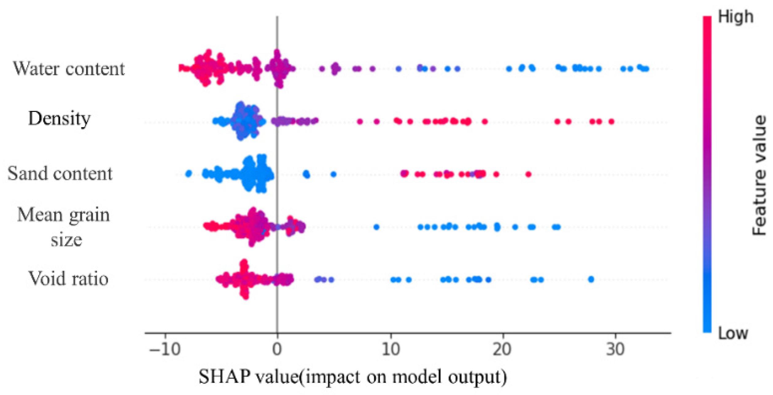
4.2. Model Interpretation

SHapley Additive exPlanations (SHAP) can be used to explain the output of the machine learning model and build an additive explanation model, and all features are regarded as “contributors.” For each predicted sample, the model produced a predicted value, and the SHAP value was the value assigned to each feature in that sample. If the i-th sample was x i , the j-th feature of the i-th sample was x i j , the predicted value of the model for the sample is y i , the baseline of the entire model (usually the mean of the target variable of the samples) is y b a s e , and then the SHAP value obeyed the following equation:
y i = y b a s e + f ( x i 1 ) + f ( x i 2 ) + + f ( x i j )
where f ( x i j ) is the SHAP value of x i j . Intuitively, it was the contribution value of the first feature in the i-th sample to the final predicted value. When f ( x i 1 ) > 0, it implied that the feature improved the predicted value, showing a positive effect; otherwise, it showed that the feature reduced the predicted value, showing a negative effect.
The characteristic factors of the prediction model of the seafloor sediment sound speed in this study were the density, water content, void ratio, sand content, and average particle size. Figure 7 shows the characteristic factors arranged from top to bottom, and the successive decrease in their contribution to the model, i.e., the contribution of the physical parameters to the sound speed in this model. The degree of influence is arranged in terms of the water content, density, sand content, average particle size, and void ratio. Moreover, Figure 7 shows that the sound speed increased with an increase in the density and sand content and decreased with an increase in the water content, void ratio, and average grain size.

5. Discussion

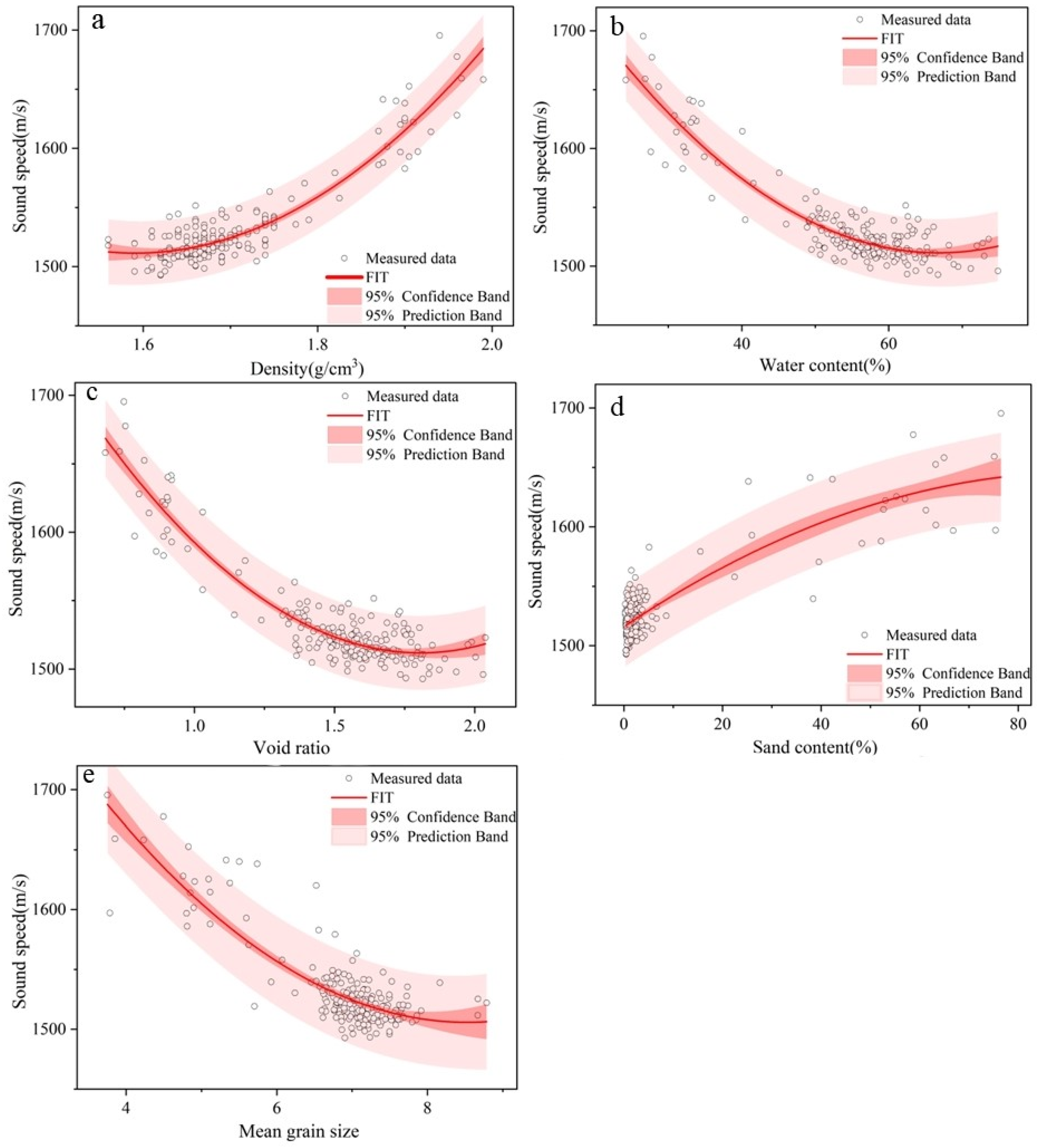
5.1. Single-Parameter Prediction Equation

Based on the 200 training sample groups, a regression analysis was performed between the sound speed and each parameter—density, water content, void ratio, sand content, and average grain size. In previous relevant studies, the traditional single parameter method for sediment sound speed is basically dominated by the unary quadratic equation [16,18,19], and in our single parameter regression analysis and comparison, the fitting effect of the single parameter using the quadratic equation is the best. For example, it is found that the fitting degree of the cubic equation established by water content and average grain size is lower than that of the quadratic equation, and the fitting degree of the cubic equation of other parameters is not improved too. So, the unary quadratic regression method was employed to obtain the single parameter equation of the sound speed prediction (Table 2). The results demonstrated that the correlation coefficient between the physical parameters and sound speed was high (R2 ≥ 0.76); the density and void ratio had the highest correlation coefficient of 0.86, followed by the water content (R2 = 0.85), sand content (R2 = 0.76), and average grain size (R2 = 0.76). Figure 8 shows the fitting curve of the sound speed and physical parameters.

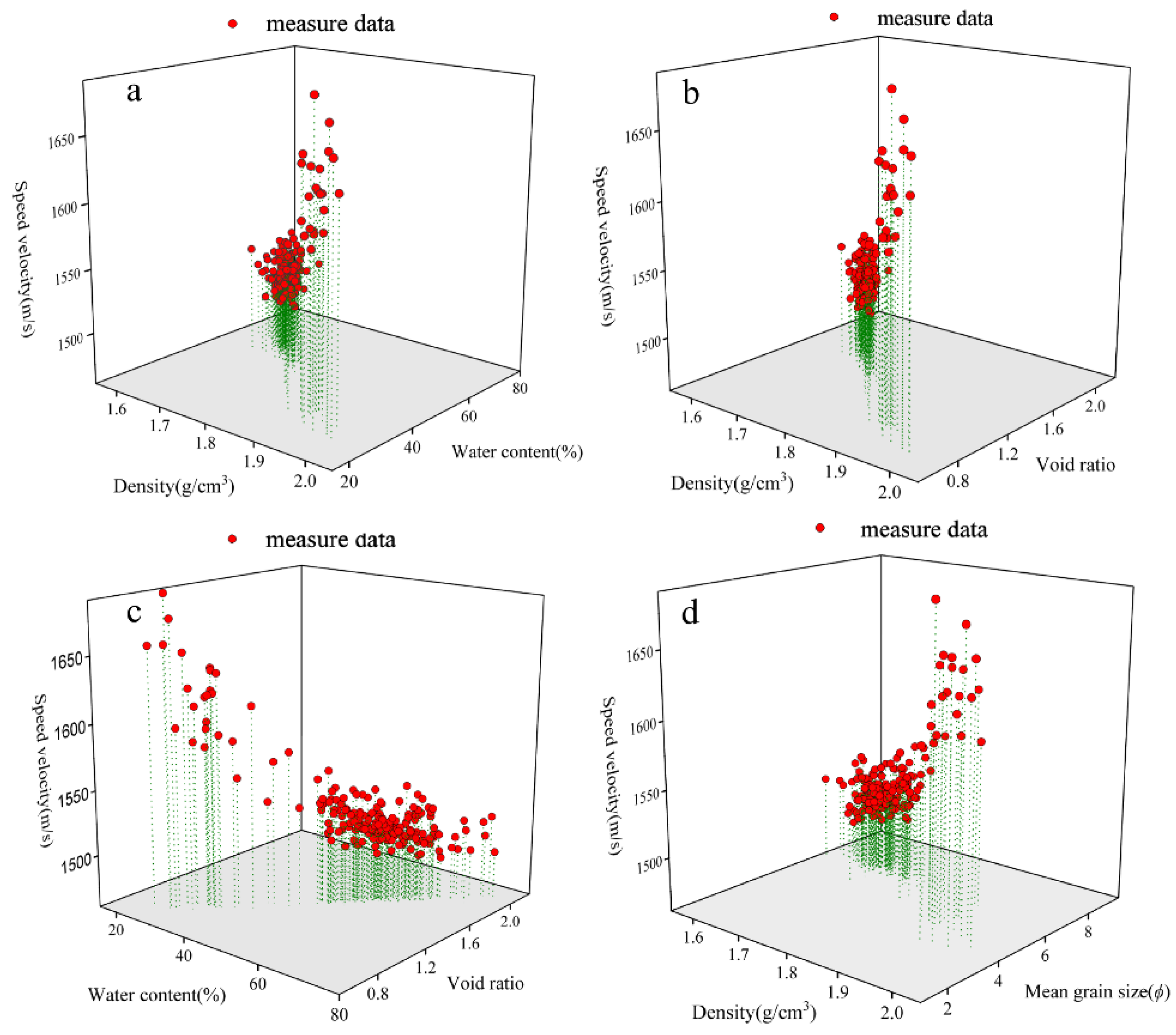
5.2. Two-Parameter Prediction Equation

Based on the 200 training sample groups, the bivariate quadratic regression prediction equation of the sound speed and two of the parameters among density, water content, void ratio, and average grain size was obtained using the principle of least square (Table 3). The results demonstrated that the correlation coefficient between the tow physical parameters and sound speed was high (R2 ≥ 0.86), The correlation coefficient of the equation obtained using the density and average grain size-based equation, density and void ratio-based equation, density and water content-based equation is 0.87, and water content and void ratio-based equation is 0.86. Figure 9 shows the 3D spatial distribution between the sound speed and parameters.

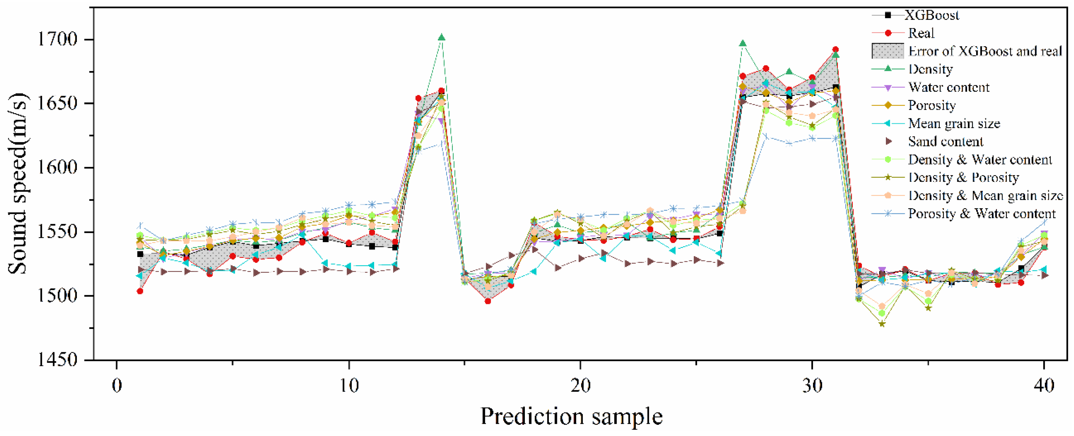
5.3. Comparison of XGBoost Prediction Models with Predictions of Single-and Two-Parameter Equations

Based on the trained XGBoost model, single-parameter prediction equations, and two-parameter prediction equations, the sound speed of the seafloor sediments was predicted for 40 groups of test samples to confirm the accuracy and superiority of the model (Figure 10). Table 4 shows the correlation error statistics between the prediction results and true values of each model. The results demonstrated that the XGBoost model exhibited the highest prediction accuracy, and the MAE, MAPE, and max absolute error are 7.99 m/s, 0.51%, and 29.27 m/s, respectively. This was followed by the density–void ratio, density, average grain size, void ratio, water content, density–water content, water content–void ratio, density–average grain size, and sand content equation. Compared with the prediction results of the traditional single- and two-parameter equations, the XGBoost model reduced the MAE and MAPE by 2.47–7.73 m/s and 0.16–0.49%, respectively. At the same time, it is found that the XGBoost model has a good performance in decreasing the max absolute error and max absolute percentage error. Compared with the traditional single- and two- parameter equation, the max absolute error and max absolute percentage error decreased by 6.54–19.56 m/s and 0.47–1.06%, respectively. Especially the max absolute error of specific density, water content, average grain size, density–water content, density–average grain size, and water content–void ratio equation decreased by more than 10 m/s. It is proven that the model has better performance in controlling errors and improving the prediction accuracy of the sediment sound speed.

6. Conclusions

Here, the sound speed prediction of seafloor sediments in the East China Sea was conducted based on the XGBoost algorithm. The optimal model super parameters were determined using 240 groups of samples from the East China Sea. Finally, the prediction accuracy of 40 groups of test samples was compared with the traditional single- and two-parameter regressional equations, and the contribution degree of the characteristic factors of the model was studied. The main conclusions of this study are as follows:
  • The XGBoost machine learning method exhibited high prediction accuracy and generalization ability when applied to the prediction of the sound speed of sediments in the East China Sea. When the n_estimator of the model was 75 and the max_depth was 5, the performance of the model was excellent, the goodness of fit (R2) was 0.923, the MAE of the training results and true values was 7.79 m/s, and the MAE of the validation results and true values was 8.96 m/s.
  • Compared with the traditional single- and two-parameter models, the seafloor sediment model exhibited a higher goodness-of-fit and prediction accuracy. The MAE, MAPE, max absolute error, and max absolute percentage error of the prediction results were 7.99 m/s, 0.51% and 29.27 m/s, 1.73%, respectively, which were 2.47–7.73 m/s, 0.16–0.49%, 6.54 m/s–19.56 m/s, and 0.47–1.06% lower than those of the traditional single- and two-parameter equations. It is proven that the model has better performance in controlling error and the prediction accuracy of the sound speed of the seafloor sediment improved.

Author Contributions

Conceptualization, G.K.; methodology, M.C.; software, X.M.; validation, M.C.; formal analysis, M.C.; investigation, X.M. and G.K.; resources and data curation, J.W.; writing—original draft preparation, M.C., Y.L. (Yuanxu Liu) and J.L.; writing—review and editing, G.K., M.C. and B.L.; visualization, G.L.; supervision, C.L. and Y.L. (Yanguang Liu). All authors have read and agreed to the published version of the manuscript.

Funding

This study was supported by the National Natural Science Foundation of China under Grant [numbers 42049902, 41676055, 41706062]; the Central Public-Interest Scientific Institution Basal Research Fund under Grant [number GY0220Q09].

Institutional Review Board Statement

Not applicable.

Informed Consent Statement

Not applicable.

Data Availability Statement

Not applicable.

Acknowledgments

Data acquisition and sample collections were supported by the National Natural Science Foundation of China Open Research Cruise (Cruise No. NORC2021-02+NORC2021-301), funded by the Shiptime Sharing Project of the National Natural Science Foundation of China. This cruise was conducted onboard R/V “XiangYangHong 18” by The First Institute of Oceanography, Ministry of Natural Resources, China.

Conflicts of Interest

The authors declare no conflict of interest.

References

  1. Pan, G. Research on the Acoustic Characteristics of Seafloor Sediments in the Northern South. China Sea; Tongji University: Shanghai, China, 2003. [Google Scholar]
  2. Jin, X.L. The development of research in marine geophysics and acoustic technology for submarine exploration. Prog. Geophys. 2007, 22, 1243–1249. [Google Scholar]
  3. Wen, D.D.; Wang, N.; Zhou, X.H. Interdisciplinary study of acoustics and marine sedimentology. Adv. Mar. Sci. 2006, 24, 392–396. [Google Scholar]
  4. Zhu, Z.Y.; Wang, D.; Zhou, J.P.; Wang, X.M. Acoustic wave dispersion and attenuation in marine sediment based on partially gas-saturated Biot-Stoll model. Chin. J. Geophys. 2012, 55, 180–188. [Google Scholar]
  5. Biot, M.A. Theory of propagation of elastic waves in a fluid-saturated porous solid: II. Higher frequency range. J. Acoust. Soc. Am. 1956, 28, 179–191. [Google Scholar] [CrossRef]
  6. Buckingham, M.J. Wave propagation, stress relaxation, and grain-to-grain shearing in saturated, unconsolidated marine sediments. J. Acoust. Soc. Am. 2000, 108, 2796–2815. [Google Scholar] [CrossRef]
  7. Buckingham, M.J. Theory of acoustic attenuation, dispersion, and pulse propagation in unconsolidated granular materials including marine sediments. J. Acoust. Soc. Am. 1997, 102, 2579–2596. [Google Scholar] [CrossRef]
  8. Buckingham, M.J. Theory of compressional and shear waves in fluidlike marine sediments. J. Acoust. Soc. Am. 1998, 103, 288–299. [Google Scholar] [CrossRef]
  9. Stoll, R.D. Sediments Acoustics; Springer: New York, NY, USA, 1989. [Google Scholar]
  10. Stoll, R.D. Acoustic waves in ocean sediments. Geophysics 1977, 42, 715–725. [Google Scholar] [CrossRef]
  11. Wood, A.B.; Lindsay, R.B. A Textbook of Sound. Phys. Today 1956, 9, 37. [Google Scholar] [CrossRef]
  12. Fu, S.S.; Tao, C.H.; Prasad, M.; Wilkens, R.H.; Frazer, L.N. Acoustic properties of coral sands, Waikiki, Hawaii. J. Acoust. Soc. Am. 2004, 115, 2013–2020. [Google Scholar] [CrossRef]
  13. Fu, S.S.; Wilkens, R.H.; Frazer, L.N. In situ velocity profiles in gassy sediments: Kiel Bay. Geo-Mar. Lett. 1996, 16, 249–253. [Google Scholar] [CrossRef]
  14. Hamilton, E.L.; Bachman, R.T. Sound velocity and related properties of marine sediments. J. Acoust. Soc. Am. 1982, 72, 1891–1904. [Google Scholar] [CrossRef]
  15. Hamilton, E.L. Prediction of in-situ acoustic and elastic properties of marine sediments. Geophysics 1971, 36, 266–284. [Google Scholar] [CrossRef]
  16. Hamilton, E.L. Geoacoustic modeling of the sea floor. J. Acoust. Soc. Am. 1980, 68, 1313–1340. [Google Scholar] [CrossRef]
  17. Guangming, K.; Yuexia, Z.; Guanbao, L.; Guozhong, H.; Xiangmei, M. Comparison on the sound speeds of seafloor sediments measured by in-situ and laboratorial technique in Southern Yellow Sea. Ocean. Technol. 2011, 30, 52–56. [Google Scholar]
  18. Kan, G.; Su, Y.; Li, G.; Liu, B.; Meng, X. The correlations between in-situ sound speeds and physical parameters of seafloor sediments in the middle area of the southern Huanghai Sea. Acta Oceanol. Sin. 2013, 35, 166–171. [Google Scholar]
  19. Dapeng, Z.; Baihai, W.; Bo, L. Analysis and study on the sound velocity empirical equations of seafloor sediments. Acta Oceanol. Sin. 2007, 29, 43–50. [Google Scholar]
  20. Orsi, T.H.; Dunn, D.A. Sound velocity and related physical properties of fine grained abyssal sediments from the Brazil Basin (South Atlantic Ocean). J. Acoust. Soc. Am. 1990, 88, 1536–1542. [Google Scholar] [CrossRef]
  21. Orsi, T.H.; Dunn, D.A. Correlations between sound velocity and related properties of glacio-marine sediments: Barents Sea. Geo-Mar. Lett. 1991, 11, 79–83. [Google Scholar] [CrossRef]
  22. Richardson, M.D.; Briggs, K.B. In situ and laboratory geoacoustic measurements in soft mud and hard-packed sand sediments: Implications for high-frequency acoustic propagation and scattering. Geo-Mar. Lett. 1996, 16, 196–203. [Google Scholar] [CrossRef]
  23. Liu, X.; Li, A.; Dong, J.; Lu, J.; Huang, J.; Wan, S. Provenance discrimination of sediments in the Zhejiang-Fujian mud belt, East China Sea: Implications for the development of the mud depocenter. J. Asian Earth Sci. 2018, 151, 1–15. [Google Scholar] [CrossRef]
  24. Xu, F.J.; Li, A.C.; Huang, J.L. Research progress in the mud deposits along the Zhemin coast of the East China Sea continental shelf. Mar. Sci. Bull. 2021, 31, 97–104. [Google Scholar]
  25. Liu, S.; Shi, X.; Fang, X.; Dou, Y.; Liu, Y.; Wang, X. Spatial and temporal distributions of clay minerals in mud deposits on the inner shelf of the East China Sea: Implications for paleoenvironmental changes in the Holocene. Quat. Intern. 2014, 349, 270–279. [Google Scholar] [CrossRef]
  26. Zhang, K.; Li, A.; Huang, P.; Lu, J.; Liu, X.; Zhang, J. Sedimentary responses to the cross-shelf transport of terrigenous material on the East China Sea continental shelf. Sediment. Geolog. 2019, 384, 50–59. [Google Scholar] [CrossRef]
  27. Lim, D.I.; Choi, J.Y.; Jung, H.S.; Rho, K.C.; Ahn, K.S. Recent sediment accumulation and origin of shelf mud deposits in the Yellow and East China Seas. Prog. Oceanogr. 2007, 73, 145–159. [Google Scholar] [CrossRef]
  28. Meng, X.M.; Liu, B.H.; Kan, G.M.; Li, G.B. An experimental study on acoustic properties and their influencing factors of marine sedi-ment in the southern Huanghai Sea. Acta Oceanol. Sin. 2012, 34, 74–83. [Google Scholar]
  29. Dong, Y.H.; Liu, L. An improved ID3 algorithm based on correlation coefficients. Comput. Eng. Sci. 2016, 38, 2342–2347. [Google Scholar]
  30. Qian, N.; Wang, X.; Fu, Y.; Zhao, Z.; Xu, J.; Chen, J. Predicting heat transfer of oscillating heat pipes for machining processes based on extreme gradient boosting algorithm. Appl. Therm. Eng. 2020, 164, 114521. [Google Scholar] [CrossRef]
  31. Shi, J.; Zhang, J. Load forecasting based on multi-model by stacking ensemble learning. Proc. CSEE 2019, 39, 4032–4042. [Google Scholar]
Figure 1. Half−matrix plot of Wilson’s correlation coefficients between the sediment sound speed and physical parameters. The first column of the matrix is the distribution of the correlation coefficient between the sound speed and each physical parameter. The redder the matrix unit, the more evident the positive correlation, and the bluer the unit, the more evident the negative correlation.
Jmse 10 01366 g001
Figure 2. Triangular sediment classification diagram. Most of the sediment in the data samples included clay silt, followed by silt sand, a small amount of silt, silty clay, and clay sand. The grey dots, red dots, and yellow triangles indicate training, validation, and test samples, respectively.
Jmse 10 01366 g002
Figure 3. The boosting algorithm principle, where m is the characteristic factor of the training sample in the model, which is each physical parameter; mij is the i-th characteristic factor of the j-th base learner; and Y represents the target value of the training sample in the model, which is the sound speed of the seafloor sediment in this study.
Jmse 10 01366 g003
Figure 4. The training process of the XGBoost model is based on the hyperparameter—n_estimator. The red and orange solid lines indicate the iterative changes in the model training error and validation result, respectively.
Jmse 10 01366 g004
Figure 5. The training process of the XGBoost model was based on the hyperparameter—max_depth. The red and orange solid lines indicate the iterative changes in the model training and validation result errors, respectively.
Jmse 10 01366 g005
Figure 6. Training and validation results of the final model. The black line is the actual measured value, the red line is the training result of 200 sets of training samples, and the brown line is the validation result of 40 sets of validation samples.
Jmse 10 01366 g006
Figure 7. SHAP value distribution of characteristic factors in the model, which shows the contribution of the sample point of each characteristic factor to the model.
Jmse 10 01366 g007
Figure 8. The single-parameter equation regression fitting of the sound speed and physical parameters: (a) density, (b) water content, (c) void ratio, (d) sand content, and (e) average grain size curves. The black hollow point, red solid line, red area, and pink area indicate the 200 training sample groups, fitted curve, confidence interval at 95%, and prediction interval at 95%, respectively.
Jmse 10 01366 g008
Figure 9. Three-dimensional scatter distribution of the sound speed and two parameters: (a) density and water content, (b) density and void ratio, (c) water content and void ratio, and (d) density and average grain size. The red dots indicate the 200 sets of training samples, and the green dotted lines indicate the projections of the dots on the coordinate plane formed by the parameters.
Jmse 10 01366 g009
Figure 10. Comparison of prediction results of 40 groups of test samples of the sediment prediction model of the XGBoost algorithm and single- and two-parameter equations. The red dotted line indicates the real sound speed value, the black dotted line indicates the prediction result of the XGBoost model, the gray area indicates the error range between the XGBoost model and the real value, and the prediction results of the single-and two-parameter equations.
Jmse 10 01366 g010
Table 1. Statistics of sound speed and physical parameters of sediments in the study area.
ρ/
( g / cm 3 )
w/
%
e S/
%
T/
%
Y/
%
Mz/
Φ
V P /
(m/s)
Max2.0074.852.0476.3079.3073.108.781695.38
Min1.5624.250.680.1010.7034.506.711492.86
Ave1.7252.071.4310.3455.157.605.91540.96
Table 2. Expressions of the single-parameter equations and fitting correlation coefficients.
Related ParametersPrediction EquationR2
ρ V P = 1141.54 ρ 2 3642.28 ρ + 4419.83 0.86
w V P = 0.088 w 2 11.74 w + 1903.64 0.85
e V P = 123.96 e 2 448.07 e + 1916.74 0.86
Mz V P = 7.90 M z 2 136.04 M z + 2086.99 0.76
S V P = 2.97 s 0.015 s 2 + 1515.95 0.76
Table 3. Expressions of double-parameter equations and fitting correlation coefficients.
Related ParametersPrediction EquationR2
ρ ,   w V P = 966.58 ρ 2 + 0.012 w 2 3123.61 ρ 1.95 w + 4111.86 0.87
ρ , e V P = 852.79 ρ 2 + 34.85 e 2 2804.28 ρ 146.72 e + 3968.22 0.87
  w , e V P = 258.35 e 2 0.099 w 2 898.03 e + 12.13 w + 1921.24 0.86
ρ ,   Mz V P = 917.54 ρ 2 + 1.3 M z 2 2904.8 ρ 18.79 M z + 3889.6 0.87
Table 4. The error analysis of the prediction results of the XGBoost model and single- and two-parameter equations.
Prediction ModelMax Absolute Error (m/s)Max Absolute
Percentage Error (%)
MAE (m/s)MAPE (%)
ρ 41.292.4910.530.67
w 42.032.7912.300.79
e 37.882.5211.970.77
Mz48.832.6510.570.67
S37.242.2015.721.00
ρ ,   w 39.362.3813.890.89
ρ ,   e 35.812.3710.460.67
w ,   e 39.392.6214.360.93
ρ , Mz41.422.7514.770.95
XGBoost29.271.737.990.51
Publisher’s Note: MDPI stays neutral with regard to jurisdictional claims in published maps and institutional affiliations.

