The Numerical Simulation and Experimental Study of Heat Flow in Seabed Sediments Based on COMSOL

Abstract

In situ electrothermal conduction heating technology refers to the setting up of a heat source directly within the sediments, using the heat conductivity of the sediments and the heat radiation of the heat source for heat transfer to achieve the in situ heating of the sediments. The in situ electrothermal conduction heating of sediments has the disadvantage of the heating equipment being easily damaged and difficult to operate, and requires the equipment to be able to withstand seawater pressure and marine corrosion. In this paper, based on the combination of numerical simulations (using COMSOL Multiphysics software) and approximate in situ electrothermal conduction heating experiments, the temperature field and other factors of sediments heated by in situ conductive heating (in a specific area) were studied to determine a numerical model for sediment heat flow in a specific area under different pressures and initial temperatures, and the correctness of the numerical model was further verified by comparative experiments. The results of this study have important implications for future studies on the actual thermal properties of sediments and even heat transfer mechanisms during gas hydrate extraction.

1. Introduction

Geothermal resources on land have been fully developed and utilized [1], yet sub-marine oil and gas resources are a huge treasure house to be explored urgently. Temperature is an important factor affecting the formation of oil and gas resources, so seafloor heat flow data are an important parameter for the comprehensive evaluation of marine oil and gas resources. In addition, the study of sub-marine heat flow is conducive to further revealing the tectonic movement laws of the oceanic crust and exploring the evolutionary history of the ocean [2]. Combined with the seafloor heat flow data and the basin evolution model, and with the help of numerical simulation methods, the temperature history experienced by each source layer can be obtained. According to the organic matter maturity model, this is expected to reveal the mature history of organic matter so as to guide the exploration and development of oil and gas [3]. Sub-marine heat flow values also represent an important basis for accurately evaluating and predicting natural gas hydrate resource potential. However, global warming may cause changes in the movement of seafloor heat flow, leading to instability and the decomposition of the fragile depositional state of natural gas hydrates, inducing geological disasters, and further increasing the instability of deep-water marine sediments [4,5]. This can even be attached to deep-sea scientific activities and research facilities, while the accelerated thawing of hydrate-laden permafrost may also pose energy and environmental challenges and exacerbate the greenhouse effect [6]. Seafloor geothermal studies include the measurement and calculation of many geothermal parameters, such as seafloor temperature, sediment thermal conductivity, and geothermal gradient.

Most seafloor sediments are tested in situ or sampled and then measured nearby. In addition, the demand for the thermal conductivity measurement of rocks in a granular or saturated state has become increasingly urgent in recent years. At the same time, as geothermal research has been gradually extended to swamp geological areas and other engineering application fields, a considerable proportion of the obtained rock samples are relatively soft mudstone, shale, weakly-cemented sandstone, etc., which cannot be processed into the rock cakes or disks required by steady-state testing methods. Therefore, the importance of the thermal conductivity measurement of loose sediments has become increasingly prominent. At present, the efficiency of the thermal conductivity measurements of seabed sediments is low, which affects the progress of marine oil and gas geological research to a certain extent. The investigation of marine oil and gas resources urgently requires us to solve related technical problems, improve work efficiency, innovate independently, and develop high-precision and high-efficiency related technologies by ourselves [7].

There are usually two forms for measuring the thermal conductivity of seabed sediments; one is in situ measurement and the other is indoor measurement. The former requires offshore operation during the measurement process, which is very difficult, and the equipment is very vulnerable to wear and tear. The latter is completed in the laboratory, which can reduce the offshore operation time and greatly reduce the risk of equipment wear. It is found that the thermal conductivity obtained by the two methods is basically the same. The measurement methods of thermal conductivity mainly include the moisture method [8] and probe test method [9]; the former is an estimated measurement value, which cannot meet the needs of increasingly sophisticated scientific research, while the latter can meet the requirements of deep-sea in situ measurement. Generally, probes are actively heated, and the heating method is typically the hot-wire method [10]. Because the water content in the sediment is large, the temperature of the probe will continue to rise due to continuous heating, resulting in the convection of the surrounding pore water, so the derived formula is difficult to apply. Therefore, the innovative heating method is the pulse heating method [11], for which the principle is to heat for a period of time at intervals, then calculate the thermal conductivity according to the time-temperature curve. A few studies also consider the frictional heat during the insertion of the probe into the deposit to calculate the thermal conductivity [12,13]. In recent years, the structure of the probe itself has been continuously improved and optimized. The thin probe can minimize the disturbance of the deposit caused by the insertion, improve the sensitivity of the thermal element to temperature changes, and reduce the error caused by the heat generated by friction, so it has more applications. Many related studies have applied the probe test method, especially for the thermal properties of natural gas hydrates [14,15,16,17]. With the development of society, box probes and dual-needle probes have also been derived, and some studies have compared the measurement results of these probes [18].

Therefore, the dual-needle probe method was adopted to systematically study the effects of different temperature and moisture content on the thermal conductivity of sediments. The numerical model was developed based on the experimental data. The numerical model includes the coupling of the thermal and flow fields, so it is simulated using the COMSOL Multiphysics software, which is based on the finite element method and realizes the simulation of real physical phenomena by solving partial differential equations. The model can better restore the thermal energy properties of sediments in a specific area. Considering the possible impact of seabed tidal currents, we also supplemented the influence of tidal flat experiments on the test data, and further improved the construction of the numerical model. In addition, the seabed sediment samples are collected based on the integrated deep-sea drilling and grabbing platform. The geographical location of the samples was 111°57′5257″ E longitude and 18°17′1906″ N latitude. The depth of the samples was 2077.30 m. The sediment samples are shown in Figure 1, the heat flow values of the marine sediments in a specific area were obtained by heating a single heat pipe under two conditions of a laboratory thermostat and a coastal shallow. Validation of the experimental heat flow values and the simulation data model further verifies the correctness of the numerical model for heat flow of seabed sediments in a specific area.

2. Design of Sediment Thermal Conductivity Test System

2.1. In Situ Heat Transfer Analysis of Sediments

Heat transfer is generally considered to be divided into three basic modes: heat conduction, heat convection, and heat radiation. Heat conduction refers to the transfer of heat between materials at different temperatures through only direct contact, without energy transfer caused by relative macroscopic motion. Heat convection is caused by macroscopic convective motion in the fluid due to the mixing of the parts at different temperatures. Heat radiation refers to the energy transfer in space by the emission of heat rays with wavelengths of 0.1–100 μm from outside of a substance [19]. In this paper, the sediments consisting of clay, sand, and mixed soils containing natural gas hydrate are studied [20,21], and because the sediments are a naturally porous type of media, containing large amounts of water in the pores, heat transfer by means of heat conduction between the sediments and heat convection between the pore water occurs under heating conditions, while heat transfer by heat radiation can be ignored during the heating process of sediments.

The temperature field refers to the temperature distribution of each point in space or the interior of an object at a certain time, and it can be expressed as:

$$T=ƒ\left(x,y,z,t\right)$$

(1)

where $T$ is temperature, $x$, $y$, and $z$ are the spatial position of the object, and $t$ is the time.

According to whether the temperature field changes with time or not, the temperature field that does not change with time represents stable heat conduction, which means that the heat conduction mode is steady heat conduction. On the contrary, the temperature field that changes with time is an unstable temperature field; for this, the heat conduction method is transient heat conduction. According to the relationship between the spatial coordinate system and the corresponding direction of temperature change, this is further divided into a one-dimensional temperature field, a two-dimensional temperature field, and a three-dimensional temperature field [22].

At the same time, in the temperature field, the surface composed of all the points with the same temperature is an isothermal surface, and there is no temperature difference on the isothermal surface, that is, there is no heat transfer, and the heat is transferred along the normal direction of the isothermal surface.

The one-dimensional, two-dimensional, and three-dimensional thermal conductivity problems follow Fourier’s law, which was proposed by the French mathematical physicist, Fourier, in 1882. The expression of Fourier’s law is shown in Equation (2).

$$q=\lambda \left(-gradT\right)=-\lambda gradT$$

(2)

where $q$ is heat transfer density in ${\mathrm{W}/\mathrm{m}}^2$, and $\lambda$ is thermal conductivity in $\mathrm{W}/\left(\mathrm{m}·\mathrm{K}\right)$.

Fourier’s law shows that the heat transfer density at each point in a uniform continuous medium is directly proportional to the temperature gradient at that point, where the negative sign indicates that the heat conduction is inversed to the temperature gradient. Thermal conductivity is a physical index to characterize the thermal conductivity of an object. Its meaning is that the heat flow density can pass through a unit temperature gradient. With the expression for temperature distribution of each part of an object at any time, it is known that the heat flow density at each point and time can be shown as Equation (3).

$$\stackrel{\rightharpoonup }{q}=\stackrel{\rightharpoonup }{q_x}+\stackrel{\rightharpoonup }{q_y}+\stackrel{\rightharpoonup }{q_z}=\left(-{\lambda }_x\frac{\partial T}{\partial x}\right)+\left(-{\lambda }_y\frac{\partial T}{\partial y}\right)+\left(-{\lambda }_z\frac{\partial T}{\partial z}\right)$$

(3)

where $\stackrel{\rightharpoonup }{q_x}$, $\stackrel{\rightharpoonup }{q_y}$, and $\stackrel{\rightharpoonup }{q_z}$ are the heat flow density of the $x$, $y$, $z$ axis of the coordinate system; ${\lambda }_x$, ${\lambda }_y$, ${\lambda }_z$ are the thermal conductivity of the $x$, $y$, $z$ axis direction, respectively, and the thermal conductivity of the isotropic body is equal in all directions.

Since the heating of the sediment is carried out by the combination of the three basic heat transfer methods mentioned above, the heat calculation requires the calculation of each of the three basic heat transfer methods separately and then the superposition of the combination. Due to the in situ sediment heating, the side and bottom surfaces of the heated sediment are in direct contact with the surrounding sediments, and the heat transfer occurs mainly through heat conduction, so the heat consumption of heat conduction is mainly considered. The surface of the sediment is in direct contact with the seawater, and there will be a mixed heat transfer of the three, mainly due to the heat convection, so the heat consumption of the heat convection is mainly considered in the calculation [23,24].

2.1.1. Calculating Heat Conduction in Cylindrical Coordinate System

When a cylindrical heating tube is used for heating, the contact thermal resistance between the heating tube and the soil and the heat conduction in the axial direction of the heating tube is ignored, and the heating tube and the heating soil can be regarded as the thermal conduction model of the cylindrical wall. When calculating the heat transfer on the side of the heated sediment, according to Fourier’s law, the heat flow calculation expression in the cylindrical coordinate system can be obtained by simplification and integration [25], as is shown in Equation (4).

$$Q=\frac{2\pi \lambda \Delta T}{\ln \left(r_2/r_1\right)}$$

(4)

where $Q$ is heat flow, $\lambda$ is thermal conductivity, $\Delta T$ is the difference between the temperature of the heat source and the minimum temperature of the edge that meets the heating requirement, $r_1$ is the radius of the heat source, and $r_2$ is the distance between the heating edge and heat source.

2.1.2. One-Dimensional Heat Conduction Flow Calculation for a Large Flat Plate

The upper surface and bottom surface of the heated soil are both planes, and their heat transfer can be considered as a one-dimensional heat conduction model problem of a large plate [26]. When calculating the heat transfer of the soil, the one-dimensional heat conduction calculation expression of a large plate is shown in Equation (5).

$$Q=-\lambda A\frac{dT}{dx}$$

(5)

where $Q$ is heat flow, $\lambda$ is thermal conductivity, and $A$ is the surface area.

2.2. Sediment Thermal Conductivity Test Experiment

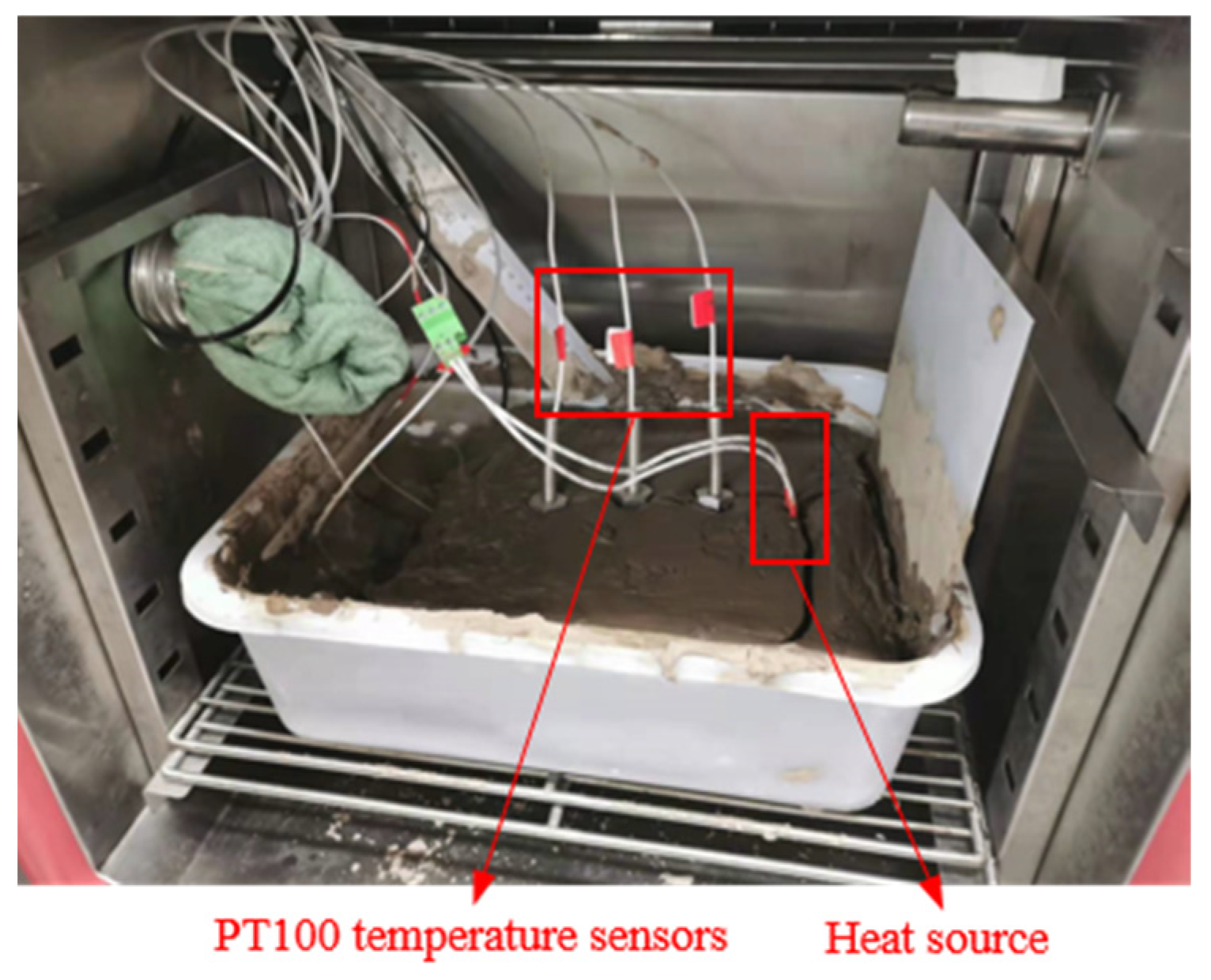
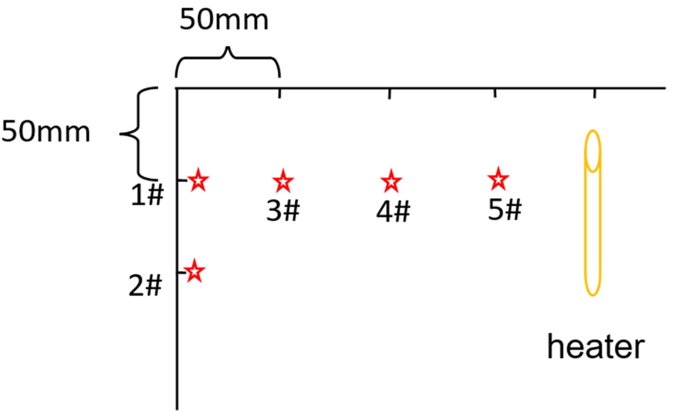
2.2.1. Test Method Construction

In order to study the effect of the thermal conductivity of the sediments from the law of the temperature rise of sediments and to facilitate subsequent heat calculations and numerical modeling, the relationship between thermal conductivity and soil moisture content needs to be studied before the in situ thermal treatment of sediments [27].

Determination of thermal conductivity by the dual-needle probe method is one of the most commonly used non-steady-state methods to measure thermal conductivity at present. Its principle is to install an electric wire inside an isotropic and homogeneous material at a homogeneous temperature to obtain the temperature change in the material with time by measuring the temperature change of the material at a certain distance from the heat source and under the condition of constant exothermic power of the heat source to obtain the size of the thermal conductivity of the test by calculation [28].

According to the specification requirements [29], the size of the specimen should be not less than 80 mm × 114 mm × 40 mm for the two boxes to place the test material in; the size of this test specimen box is 110 mm × 190 mm × 50 mm, as shown in Figure 2. The heat source material adopts a resistance wire with a diameter of 0.3 mm and a length of 200 mm; the heat source adopts a constant voltage DC power supply, the voltage and current control range is 30 V/5 A, and the control accuracy is 0.01. The temperature sensor adopts Ф4 × 30 mm PT100, the accuracy of the sensor is 0.1, and the temperature collector adopts a multi-channel automatic temperature collection system. The test process is based on the requirements of the specification, the specific steps will not be repeated.

The measured temperature data will be processed at a time interval of 30 s, with the temperature rise law curve of the heat wire obtained, which is calculated according to the calculation formula of thermal conductivity, as shown in Equation (6).

$$\lambda =\frac{P}{4\pi LK}$$

(6)

where $P$ is the heating power of the heat wire, $L$ is the length of the heat wire, $K$ is the slope of the curve of the logarithm of heating time versus temperature rise.

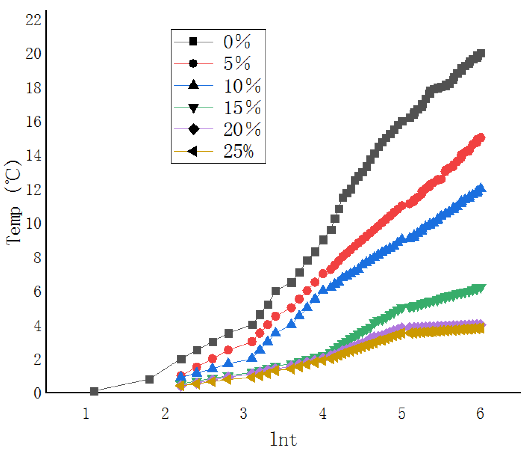
2.2.2. Analysis of Results

The soil samples were dried in an oven, and samples with differing moisture contents of 0%, 5%, 10%, 15%, 20%, and 25% were prepared by adding different amounts of water. The temperature rise data of these samples were tested. The test results are shown in Figure 3; the analysis of the figure shows that the water content has a significant impact on the temperature rise of the heat-line. Generally speaking, it can be seen that the lower the soil water content, the faster the temperature rise of the heat-line is, and vice versa. With a 20% water content, the temperature rise of the heat-line slows down with the increase in water content, which is mainly due to the fast temperature loss of the heat-line due to the presence of water. When the water content reaches 20%, the temperature rising speed of the heat-line is the slowest, that is, when the water content is greater than this value, the temperature rising speed no longer slows with the increase in water content but increases faster with the increase in water content.

The slope of the fitting curve is obtained by implementing a linear fit to the data in Figure 3 with the help of ORIGIN, and then bringing it into Equation (6) for calculation to obtain the thermal conductivity of the sediment samples. The calculated results are shown in

Table 1. Thermal conductivity of sediments with different water content.

Moisture Content	U (V)	I (A)	L (m)	$\mathbf{K}(\mathbf{ln}\mathit{t}-\mathit{\Delta }\mathit{T})$	λ (W/(m·K))
0%	4	1	0.22	5.0012	0.289
5%	4	1	0.22	3.8501	0.3759
10%	4	1	0.22	3.1253	0.4631
15%	4	1	0.22	1.7584	0.8232
20%	4	0.9	0.22	0.8841	1.4736
25%	4	0.9	0.22	1.0342	1.2597

.

Analyzing the relationship between soil moisture content and thermal conductivity in Figure 4, it can be found that the thermal conductivity of the pulverized clay soil becomes larger with an increase in moisture content. The thermal conductivity becomes larger with the increase in moisture content when the content is within 20%, and the thermal conductivity tends to decrease when the content is larger than this value. This is mainly because, within 20% moisture content, the soil mostly transfers heat through the soil particles and less through the water in the soil. When the moisture content is higher than this value, the heat transfer form of the soil turns to mainly heat transfer by the water in the soil and soil particles together, which means that the thermal conductivity of the soil is no longer significantly affected by the moisture content.

The relative uncertainty of the thermal conductivity measurements of those samples with 0%, 5%, 10%, 15%, 20% and 25% moisture content, was 5.52%, 7.17%, 8.83%, 15.70%, 31.22%, and 26.69%, respectively. The calculation process is shown in Appendix A.

3. Simulation

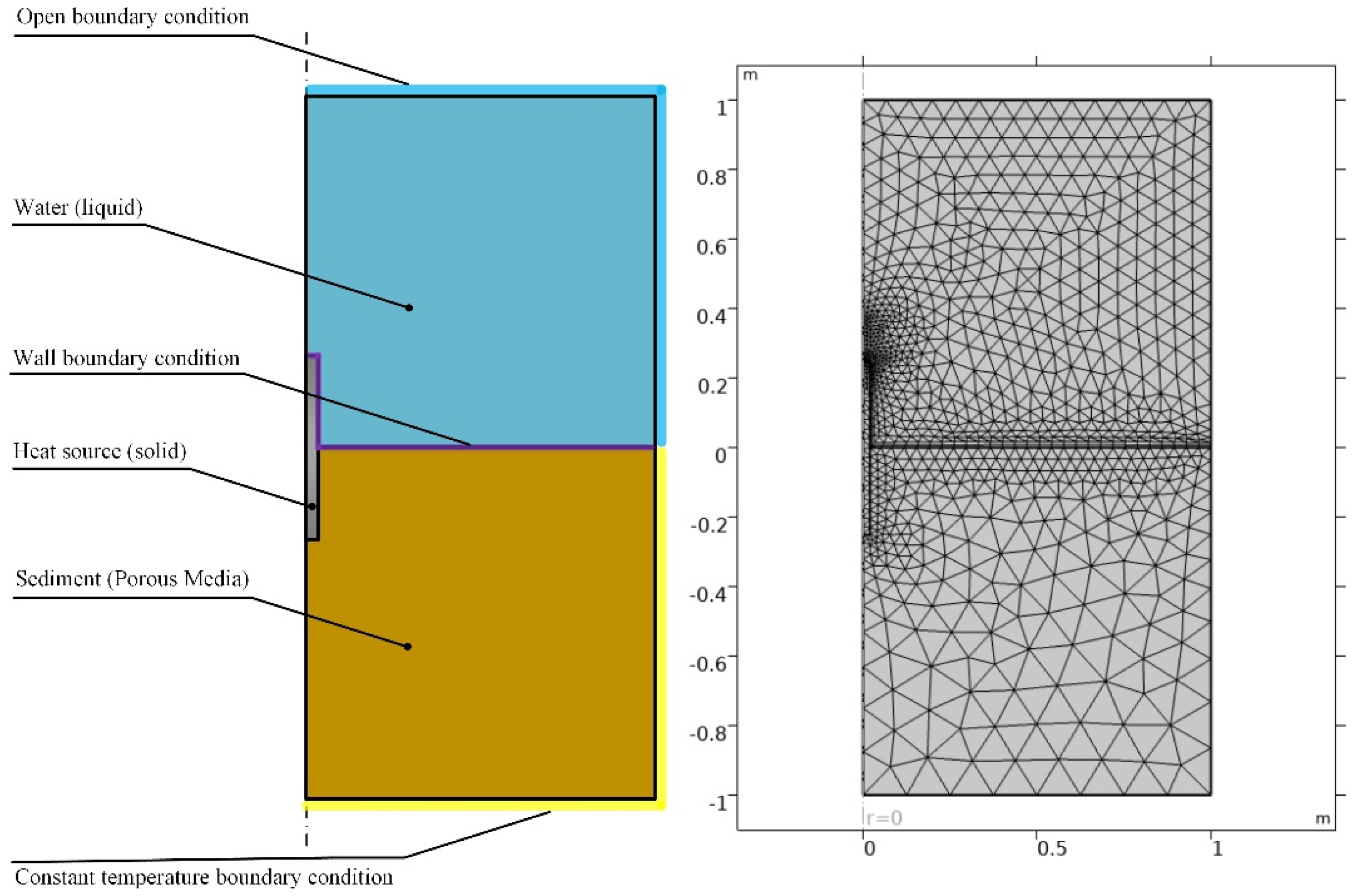
3.1. Finite Element Model

The whole model is mainly divided into three parts: the heat source, sediment, and water. The heat transfer in the fluids and solids interface is enabled throughout the model, and the heat transfer in the porous media interface is used in the sediment part. Due to the strong coupling relationship between the thermal field and the flow field in the liquid, the laminar flow interface is introduced to analyze the thermal field and the flow field at the same time. The boundary conditions and meshing of the simulation model are shown in Figure 5.

The following simplification conditions are used to simplify the model:

(1)

The thermal deformation of the soil during the heating process is ignored;

(2)

Contact thermal resistance between heating the heat source and soil is ignored;

(3)

Changes in basic property parameters during soil heating are ignored and the soil is considered to be homogeneous and isotropic, so the physical parameters of the porous medium (density, heat capacity, thermal conductivity, etc.) are assumed to be constant;

(4)

The porous medium is assumed to be homogeneous, isotropic, and fully saturated;

(5)

The thermally-induced pore flow in porous media is described by Darcy’s law [30].

The simulation area is set as a cylinder with a radius of 1 m and a height of 2 m, which includes porous media sediments with a height of 1 m and seawater covering the sediments with a height of 1 m. The sediment boundary condition is the ambient temperature (4 °C on the seabed, and the tidal flat is set according to the measured temperature); the seawater boundary is set as an open boundary, and the upstream temperature is the ambient temperature (4 °C on the seabed, and the tidal flat is set according to the measured temperature), that is, the radius of the affected area of the heating pipe is less than 1 m. A cylinder with a radius of 0.002 m and a height of 0.4 m is used to simulate the soil-heating heat source. The constant power heating element is embedded in a saturated porous medium. Based on the saturated porous medium model with a constant power heat source, the mechanism of conduction heat-transfer and convection heat-transfer in a saturated porous medium is analyzed by simulating the temperature distribution in the research domain, considering heat-flow coupling.

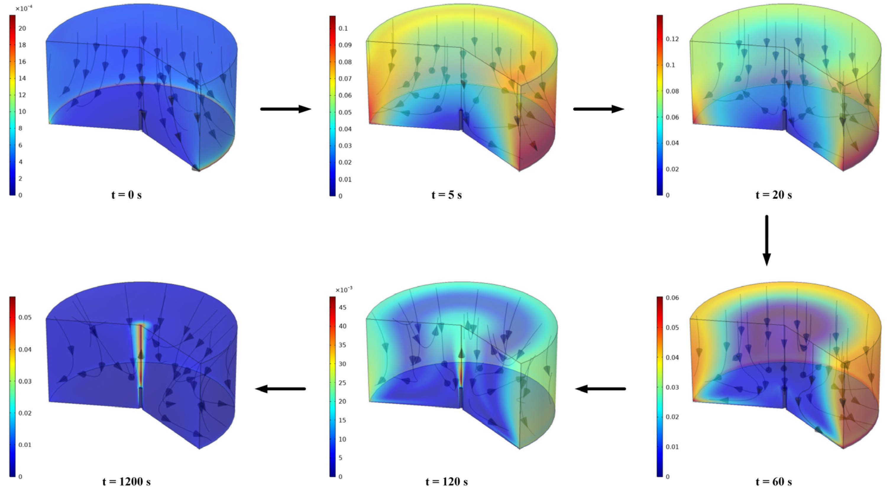
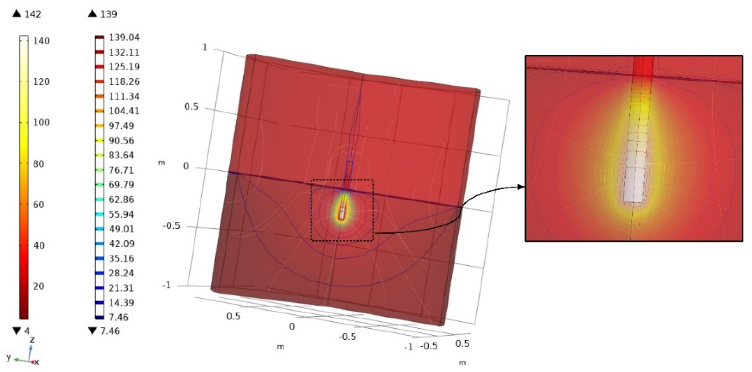
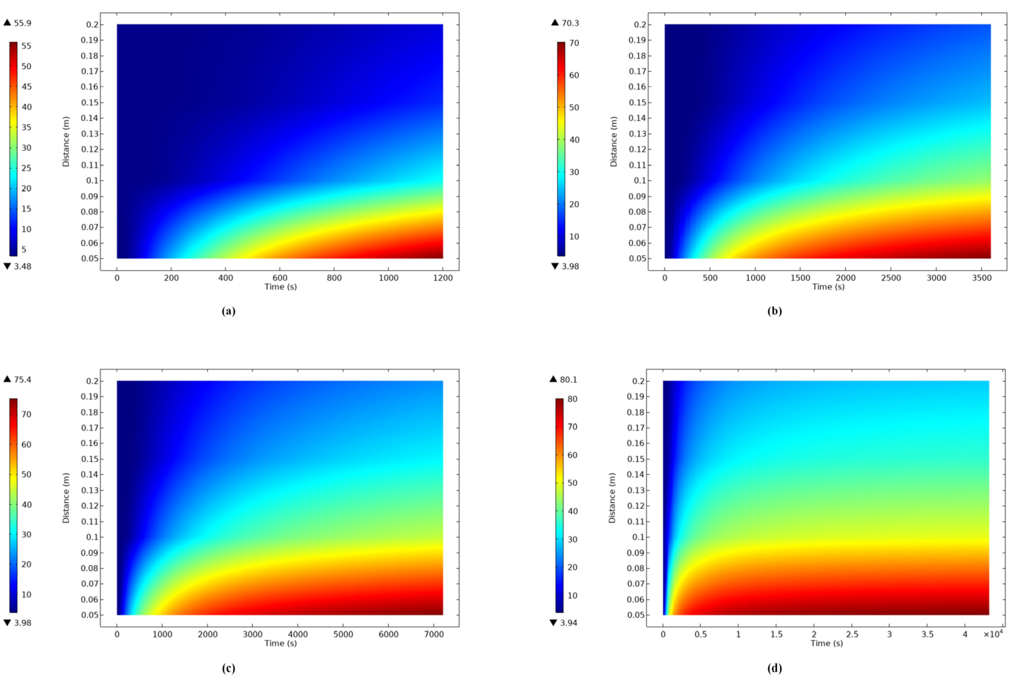
3.2. Simulation Analysis and Discussion

Figure 6 shows the change in the flow velocity field in the water area with heating time. In the initial state, the heat source is not turned on, and the seawater only tends to flow downward under the action of gravity, and the flow velocity is almost zero. The field state is stable, and only the high-temperature seawater flows upward.

Figure 7 shows the distribution of the temperature field after 12 h of heating. The isotherm is denser near the heat source in the sediment and sparser in the water body. The maximum temperature at the heat source can reach 142 °C. The temperature distribution in the water body is relatively uniform, but in the sediment, there is a great change with the increase in distance away from the heat source. This is because the thermal conductivity of seawater is dozens of times that of the sediment [31], and the sediment has a strong inhibitory effect on heat diffusion. Therefore, if the deposit needs to be heated to a higher temperature, the power of the heat source can be increased, or the number of heat sources can be increased. However, in practical applications, increasing the power of a single heat source will greatly increase the cost, and multiple-line heat sources will cause an uneven temperature in the area to be heated. Other shapes of heat sources can be considered, such as annular heat sources [32].

In order to visually observe the temperature distribution in the sediment, temperature probes were placed at 0.05 m, 0.1 m, 0.15 m, and 0.2 m from the heat source, respectively. Figure 8 shows the fitted image according to the change in the temperature at the probe, with heating time. The horizontal axis is the heating time, and the vertical axis is the distance from the heat source. Figure 8a–d simulate the cases where the total heating time was 1200 s, 60 min, 120 min, and 12 h, respectively. It can be seen from the figure that, after the heating time exceeds 200 min, the temperature of the sediment within 0.1 m from the heat source tends to be stable, and the heat conduction reaches an equilibrium state. The farther away from the heat source, the later the sediment heat transfer reaches an equilibrium state.

In order to facilitate the application of the simulation results to engineering, the relationship between the temperature and the heating time was fitted for the working condition, with a heating time of 120 min, as shown in Figure 9 below. The points at a distance of 0.05 m, 0.1 m, 0.15 m, and 0.2 m from the heat source were selected, respectively, and the relationship between temperature and time was fitted to an 8th-degree polynomial as shown in Equation (7). The coefficients and coefficients of determination are shown in

Table 2. Fitting results.

Distance (m)	0.05	0.1	0.15	0.2
p1	−1.603 × 10−13	2.608 × 10−13	8.317 × 10−14	1.993 × 10−14
p2	9.218 × 10−11	−1.366 × 10−10	−4.59 × 10−11	−1.143 × 10−11
p3	−2.244 × 10−8	2.963 × 10−8	1.065 × 10−8	2.794 × 10−9
p4	3.013 × 10−9	−3.434 × 10−6	−1.346 × 10−6	−3.803 × 10−7
p5	−0.000244	0.0002279	0.0001003	3.14 × 10−5
p6	0.01227	−0.00849	−0.004403	−0.001581
p7	−0.3827	0.15	0.102	0.04351
p8	7.31	0.04844	−0.5358	−0.2418
p9	−5.342	3.016	4.605	4.298
Coefficients of Determination (%)	99.95	99.97	99.99	99.99

. The trend of this data curve is consistent with the temperature change of resistively heated porous media [33].

$$f(x)=p_1{x}^8+p_2{x}^7+p_3{x}^6+p_4{x}^5+p_5{x}^4+p_6{x}^3+p_7{x}^2+p_8{x}^1+p_9$$

(7)

4. Experimental Verification

4.1. Incubator Experiment

In order to verify the accuracy of the numerical model for the heat flow of marine sediments in a specific area at an initial temperature of approximately 4 °C (in a deep-sea environment), a sediment heating experiment was performed in a laboratory incubator. The heating experiment for the (laboratory) constant temperature box is shown in Figure 10. In this laboratory simulation experiment, the VGGDWS-100-type test box, with a balanced temperature and humidity control, was used. The adjustable temperature range of the test box is −20–150 °C, and the adjustable humidity range is 30–98% RH. The acquisition accuracy of the device is 0.2%FS, and the temperature sensor is a PT100 with an accuracy of 0.1%FS. The heating probe adopts an electric heating tube with a constant power output of 150 W and a power supply voltage of DC24V. The outer dimension of the heating probe is Ф12 × 60 mm. The sediments recovered from the South China Sea through the integrated drilling and grasping equipment were placed in the test box, and the upper surface of the sediments was covered with a layer of overlying water in the area where the recovered sediments were located. The arrangement of the heating probes and temperature sensors is shown in Figure 11. The red star is the position of the temperature sensor. The position interval of each temperature sensor is 50 mm, and the position of the right heating probe and the temperature sensor are separated by 50 mm.

The data obtained from the experiment and the graphs were drawn, as shown in Figure 12. The temperature in the incubator gradually drops from room temperature to a set temperature value of 4 °C. At this time, the heater is started, and the temperature values of the five nodes gradually increase under the action of the heater. Node 5 was closest to the heating probe, so the temperature rises the fastest. The rate of temperature rise decreases in the order of node 5 → node 4 → node 3 → node 1 → node 2. During the period from 300 min to 500 min, the temperature pulse value appeared because the liquid level of the water overlying the sediment was too low, and part of the sediment was exposed to the air. After adding the overlying water over the sediment, the temperature decreased and gradually became stable, which was consistent with the simulation results of the model.

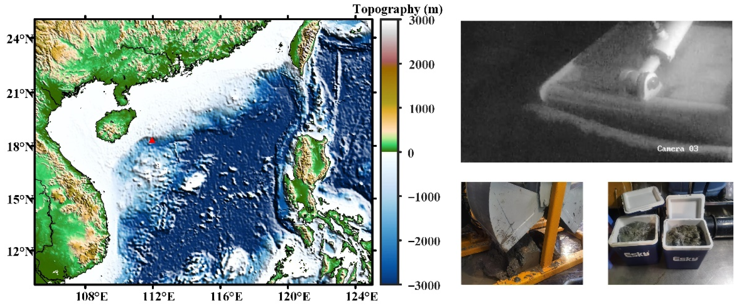
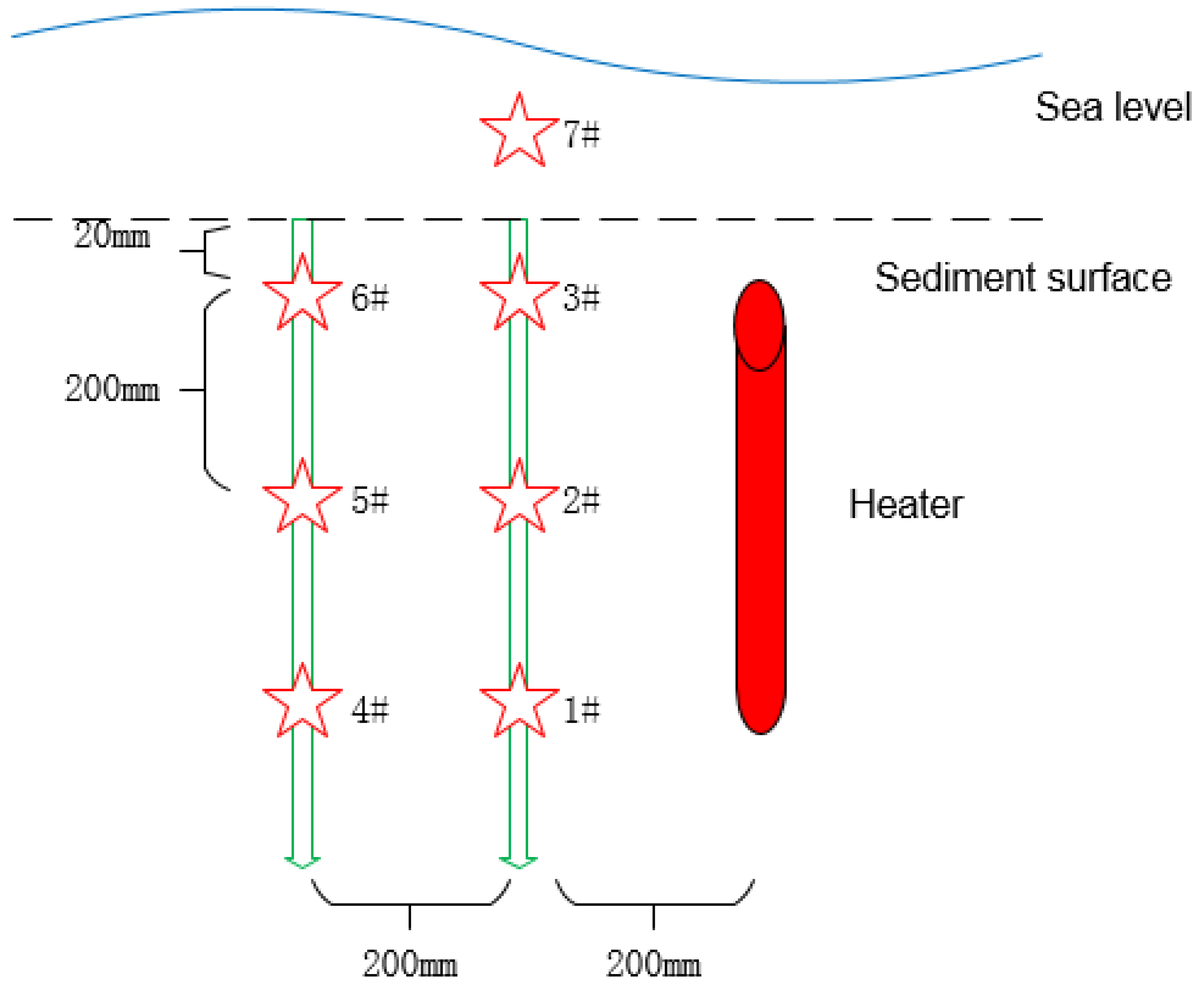
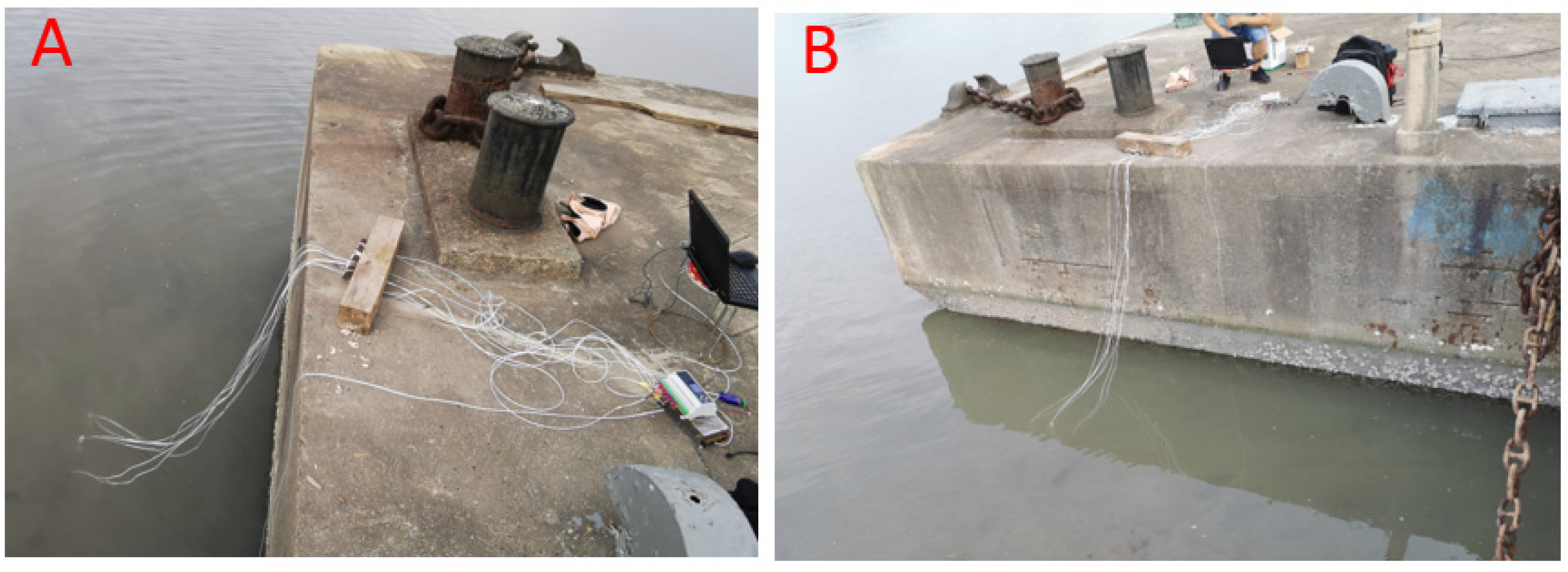
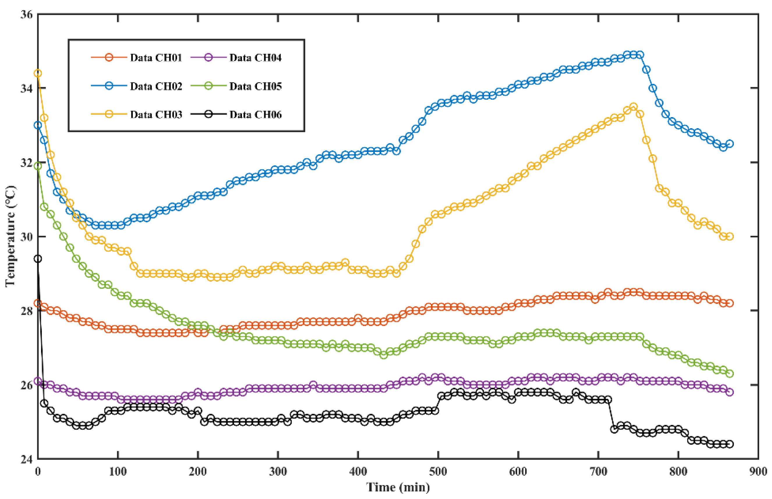
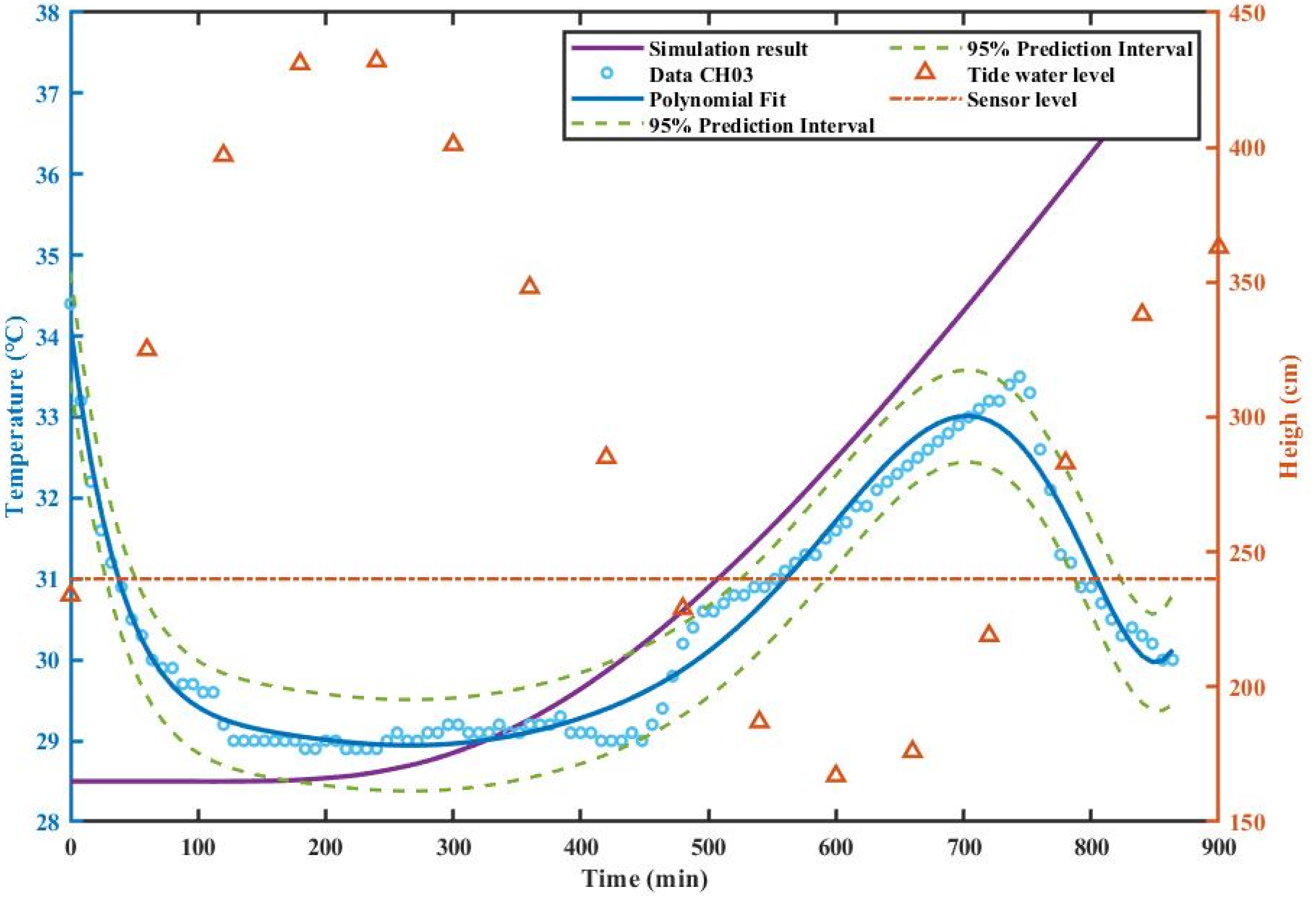
4.2. Experiment on the Shallows by the Sea

In order to further verify the accuracy of the numerical model for the heat flow of the sediments in a certain area of marine sediments in an environment where the seawater is approximately in situ, a seaside tidal flat experiment was carried out. Before the shoal test, the marine sediments obtained by the mobile platform were transferred to the tidal flat to be tested. The arrangement of the heating probe and the temperature acquisition sensor is shown in Figure 13. The whole process of the seaside shoal experiment started at 5:00 pm the day before and ended at 8:00 am the next day. During the process, it experienced two high-tide levels and one low-tide level. The seaside shoal experiment is shown in Figure 14.

The data analysis of the seaside shoal experiment is shown in Figure 15. The temperature values for the six nodes, at the beginning of the heating, all decreased because the temperature of the sediments gradually increased from bottom to top under the action of sunlight before the tidewater submerged the shoal sediments. When the seawater submerged and began to gradually heat up, there was a downward trend in the temperature of all the nodes due to the lower seawater temperature. After heating for a period of time, the node temperature increased with the increase in heating time.

Figure 16 shows the relationship between the temperature collected at node 3 and the seawater tide level. When the tide ebbs and failed to submerge the heating probe and the temperature acquisition device, there was a trend of node temperature rise, and the temperature rise of node 2 and node 3 is more obvious. When the tide rises again and the water submerged the heating probe and the temperature acquisition node, the temperature of the acquisition node decreased and became stable. The sediment was heated from the initial temperature to a steady state, and the temperature rise curve maintains the same trend as the simulation model. This verifies that the initial conditions, boundary conditions, and other parameters of the model are reasonably configured, which is beneficial to the optimization of the subsequent model and provides a basis for further research in the future.

5. Conclusions

In this study, the dual-needle probe method was adopted to measure thermal conductivity. A number of experiments were performed on the variations of thermal conductivity of sediments at different temperatures and moisture contents while maintaining the sediment samples under approximate in situ sampling pressure conditions. Based on the experimental data, a numerical model for simulation was constructed in COMSOL Multiphysics. The experiments show that the moisture content has a significant effect on the temperature rise of the heat source. The numerical model considers the coupling of the thermal and flow fields, so the prediction results of the model are basically consistent with the experimental tests, and the results of the tidal flat experiments further verified the correctness of the numerical model. The results of this study are beneficial to the calculation of the thermal conductivity of deep-sea sediments and have long-term significance for the massive exploitation of natural gas hydrates.

References

1. Aguilar-Ojeda, J.A.; Campos-Gaytán, J.R.; Villela, A.; Herrera-Oliva, C.S.; Ramírez-Hernández, J.; Kretzschmar, T.G. Understanding hydrothermal behavior of the maneadero geothermal system, Ensenada, Baja California, Mexico. Geothermics 2020, 89, 101985. [Google Scholar] [CrossRef]
2. Stein, C.A. Geophysical Heat Flow; Univ Illinois: Chicago, IL, USA, 2019; pp. 1–8. [Google Scholar]
3. Miao, W. Development of Data Acquisition and Process Software for Multi-Channel Thermal Conductivity Meter. Ph.D. Thesis, China University of Geosciences, Beijing, China, 2011. [Google Scholar]
4. Kvenvolden, K.A. Potential effects of gas hydrate on human welfare. Proc. Natl. Acad. Sci. USA 1999, 96, 3420–3426. [Google Scholar] [CrossRef] [PubMed]
5. Hornbach, M.J.; Harris, R.N.; Phrampus, B.J. Heat flow on the U.S. beaufort margin, arctic ocean: Implications for ocean warming, methane hydrate stability, and regional tectonics. Geochem. Geophys. Geosyst. 2020, 21, e2020GC008933. [Google Scholar] [CrossRef]
6. Farahani, M.V.; Hassanpouryouzband, A.; Yang, J.; Tohidi, B. Insights into the climate-driven evolution of gas hydrate-bearing permafrost sediments: Implications for prediction of environmental impacts and security of energy in cold regions. RSC Adv. 2021, 11, 14334–14346. [Google Scholar] [CrossRef] [PubMed]
7. Chen, G. Research on Several Key Technologies of Sediment Thermal Conductivity Meter. Ph.D. Thesis, China University of Geosciences, Beijing, China, 2008. [Google Scholar]
8. Gerard, R.; Langseth, M.G.; Ewing, M. Thermal gradient measurements in the water and bottom sediment of the western Atlantic. J. Geophys. Res. Earth Surf. 1962, 67, 785–803. [Google Scholar] [CrossRef]
9. Von Herzen, R.; Maxwell, A.E. The measurement of thermal conductivity of deep-sea sediments by a needle-probe method. J. Geophys. Res. Earth Surf. 1959, 64, 1557–1563. [Google Scholar] [CrossRef]
10. Sclater, J.G.; Corry, C.E.; Vacquier, V. In situ measurement of the thermal conductivity of ocean-floor sediments. J. Geophys. Res. Earth Surf. 1969, 74, 1070–1081. [Google Scholar] [CrossRef]
11. Lister, C.R.B. Measurement of in situ sediment conductivity by means of a bullard-type probe. Geophys. J. Int. 1970, 19, 521–532. [Google Scholar] [CrossRef]
12. Lee, T.-C.; Von Herzen, R.P. In situ determination of thermal properties of sediments using a friction-heated probe source. J. Geophys. Res. Earth Surf. 1994, 99, 12121–12132. [Google Scholar] [CrossRef]
13. Lee, T.-C.; Duchkov, A.D.; Morozov, S.G. Determination of thermal conductivity and formation temperature from cooling history of friction-heated probes. Geophys. J. Int. 2003, 152, 433–442. [Google Scholar] [CrossRef] [Green Version]
14. Duchkov, A.D.; Manakov, A.Y.; Kazantsev, S.A.; Permyakov, M.E.; Ogienko, A.G. Thermal conductivity measurement of the synthetic samples of bottom sediments containing methane hydrates. Izv. Phys. Solid Earth 2009, 45, 661–669. [Google Scholar] [CrossRef]
15. Yang, L.; Zhao, J.F.; Wang, B.; Liu, W.G.; Yang, M.J.; Song, Y.C. Effective thermal conductivity of methane hydrate-bearing sediments: Experiments and correlations. Fuel 2016, 179, 87–96. [Google Scholar] [CrossRef]
16. Chuvilin, E.; Bukhanov, B. Thermal conductivity of frozen sediments containing self-preserved pore gas hydrates at atmospheric pressure: An experimental study. Geosciences 2019, 9, 65. [Google Scholar] [CrossRef]
17. Farahani, M.V.; Hassanpouryouzband, A.; Yang, J.H.; Tohidi, B. Heat transfer in unfrozen and frozen porous media: Experimental measurement and pore-scale modeling. Water Resour. Res. 2020, 56, e2020WR027885. [Google Scholar] [CrossRef]
18. Kim, D.; Oh, S. Measurement and comparison of thermal conductivity of porous materials using box, dual-needle, and single-needle probe methods—A case study. Int. Commun. Heat Mass Transf. 2020, 118, 104815. [Google Scholar] [CrossRef]
19. Wang, B. Engineering Heat and Mass Transfer; Science Press: Beijing, China, 2015. [Google Scholar]
20. Klauda, J.B.; Sandler, S.I. Global distribution of methane hydrate in ocean sediment. Energy Fuels 2005, 19, 459–470. [Google Scholar] [CrossRef]
21. Wang, S.; Lu, X.; Zhang, X. Advances in the laboratory apparatus and research on mechanical properties of gas hydrate sediment. J. Exp. Mech. 2009, 24, 413–420. [Google Scholar]
22. Chuvilin, E.; Bukhanov, B. Effect of hydrate formation conditions on thermal conductivity of gas-saturated sediments. Energy Fuels 2017, 31, 5246–5254. [Google Scholar] [CrossRef]
23. Muraoka, M.; Ohtake, M.; Susuki, N.; Yamamoto, Y.; Suzuki, K.; Tsuji, T. Thermal properties of methane hydrate-bearing sediments and surrounding mud recovered from nankai trough wells. J. Geophys. Res. Solid Earth 2014, 119, 8021–8033. [Google Scholar] [CrossRef]
24. Kim, Y.; Yun, T. Thermal conductivity of methane hydrate-bearing Ulleung basin marine sediments: Laboratory testing and numerical evaluation. Mar. Pet. Geol. 2013, 47, 77–84. [Google Scholar] [CrossRef]
25. Cortes, D.; Martin, A.; Yun, T.; Francisca, F.; Santamarina, J.; Ruppel, C. Thermal conductivity of hydrate-bearing sediments. J. Geophys. Res. Earth Surf. 2009, 114, B11103. [Google Scholar] [CrossRef] [Green Version]
26. Munholland, J.L.; Mumford, K.G.; Kueper, B.H. Factors affecting gas migration and contaminant redistribution in heterogeneous porous media subject to electrical resistance heating. J. Contam. Hydrol. 2016, 184, 14–24. [Google Scholar] [CrossRef] [PubMed]
27. Yiqing, W. Study on High Temperature Treatment of Silty Clay Based on In-Situ Electrical Thermal Conductivity; Dalian Maritime University: Dalian, China, 2020. [Google Scholar]
28. Rupeng, W. Experimental Study and Prediction Model of Thermal Conductivity of Hydrate-Bearing Sediment; Dalian University of Technology: Dalian, China, 2019. [Google Scholar]
29. GB/T 10297-1988; Test Method for Thermal Conductivity of Nonmetal Solid Materials—Hot-Wire Method. Standards Press of China: Beijing, China, 2015.
30. Fu, G.; Yang, Y. A hybrid-mixed finite element method for single-phase darcy flow in fractured porous media. Adv. Water Resour. 2022, 161, 104129. [Google Scholar] [CrossRef]
31. Zhang, X.; Kong, G.-Q.; Li, H.; Wang, L.; Yang, Q. Thermal conductivity of marine sediments influenced by porosity and temperature in the South China Sea. Ocean Eng. 2022, 260, 111992. [Google Scholar] [CrossRef]
32. Gallo-Villanueva, R.; Perez-Gonzalez, V.; Cardenas-Benitez, B.; Jind, B.; Martinez-Chapa, S.O.; Lapizco-Encinas, B. Joule heating effects in optimized insulator-based dielectrophoretic devices: An interplay between post geometry and temperature rise. Electrophoresis 2019, 40, 1408–1416. [Google Scholar] [CrossRef] [PubMed]
33. Hassanzadeh, H.; Harding, T. Analysis of conductive heat transfer during in-situ electrical heating of oil sands. Fuel 2016, 178, 290–299. [Google Scholar] [CrossRef]
Figure 1. Schematic diagram of sediment samples.
Jmse 10 01356 g001
Figure 2. Experimental photo of the thermal conductivity measurement.
Jmse 10 01356 g002
Figure 3. The relationship between the logarithm of the heating time and temperature rise for different moisture content.
Jmse 10 01356 g003
Figure 4. The curve between soil moisture content and thermal conductivity.
Jmse 10 01356 g004
Figure 5. The schematic of the boundary conditions and meshing of the simulation model.
Jmse 10 01356 g005
Figure 6. Simulation results for flow velocity field evolution.
Jmse 10 01356 g006
Figure 7. 12 h temperature field simulation results.
Jmse 10 01356 g007
Figure 8. Table of the surface of the probe temperature: (a) simulation with heating time of 1200 s; (b) simulation with heating time of 60 min; (c) simulation with heating time of 120 min; (d) simulation with heating time of 12 h.
Jmse 10 01356 g008
Figure 9. Fitting curve for the temperature-time relationship.
Jmse 10 01356 g009
Figure 10. Heating experiment in the laboratory incubator. (A) overview photo of experiment in the laboratory incubator; (B) photo of sensor arrangement in incubator.
Jmse 10 01356 g010
Figure 11. Arrangement of heating source and temperature sensors in the incubator. 1#–5# in the figure represent temperature sensors 1–5.
Jmse 10 01356 g011
Figure 12. Temperature vs. time curves of sensor nodes in incubator.
Jmse 10 01356 g012
Figure 13. Arrangement of heating source and temperature sensors in the seaside shoal. 1#–7# in the figure represent temperature sensors 1–7.
Jmse 10 01356 g013
Figure 14. The experimental scene of the seaside shoal. (A) photo of the experimental installation on the shore; (B) photo of sensor and probe placement.
Jmse 10 01356 g014
Figure 15. Temperature vs. time curves of sensor nodes at seaside shoal.
Jmse 10 01356 g015
Figure 16. The relationship between the temperature value of node 3 and seawater tide level.
Jmse 10 01356 g016