Dynamic Lifetime Prediction of Fishing Nets Based on the Model of Wave Return Period and Residual Strength

Abstract

The classical cumulative damage method based on the S-N curve or crack growth model is unrealistic for predicting the lifetime of fishing nets under actual service conditions. In this paper, a novel and practical method based on the wave return period model and residual strength model is presented to estimate the dynamic lifetime of fishing nets under different numbers of damaged netting bars. The tension distribution rules, dangerous breakage zones, damage-developing-paths, and breakage patterns of two types of tensioned nettings are calculated using the commercial software RIFLEX. The most dangerous breakage zones appear in the areas near the midpoint of the upper fixing boundary side for both square mesh and diamond mesh netting. The tension distribution of diamond mesh netting is more uniform than that of square mesh netting, which implies that diamond mesh is more durable than square mesh. The dynamic lifetime prediction shows that the netting will be damaged more and more quickly after its initial fracture. Relative dynamic lifetime curves provide a way to forecast the subsequent damage time according to the net’s initial fracture lifetime. Adjusting the installation angle of the polygon cage can reduce the maximum tension of a fishing net under the wave load, thus increasing the lifetime of the fishing net.

1. Introduction

Fishing nets are mainly composed of high-molecular chemical synthetic fibers, such as polyamide (PA), polyester (PES), polyethylene (PE), high-density polyethylene (HDPE), ultra-high-molecular weight polyethylene (UHMWPE), etc. [1]. Large deep-sea aquaculture cages’ fishing nets mainly use ultra-high-molecular weight polyethylene (UHMWPE) fibers [2]. Generally, fishing nets have a short lifespan and are easily corroded, squeezed, and worn, and thus often regarded as consumables [3]. Few studies have focused on the net’s damage patterns and lifespan prediction. After Norway’s “Ocean Farm 1” and China’s “Deep Blue 1” deep-sea net cages were put into use in 2017 and 2018, respectively, the deep-sea net cage has gradually become a hotspot in research and industrial development. As these cages usually work in an open ocean, typhoons and giant waves often threaten the net cages, and the nets are more likely to be damaged by wave forces. The net-breaking accident of a deep-sea cage has brought widespread anxieties about the safety of deep-sea aquaculture net cages. Therefore, it is urgent to find a feasible method to predict the lifetime of fishing nets. The lifetime prediction of fishing nets is a new research field, and there is no mature method used at present.

Furthermore, under deep-sea conditions, slight damage to the net is not easy to find in time to repair immediately. Nonetheless, the fishing net has to keep working despite fractures that may occur. According to the research interview of Lin [4], a technologist at a fishing net factory in China, once some netting twines are damaged, the damaged area will expand more and more quickly, and this is most notable for knotless nets. Therefore, the duration for which the net can continue to operate within a functional range of damage is also a critical concern. A study of the dynamic lifetime prediction of consequential damages is necessary. This question proposes a new research field.

Before solving the issue of dynamic lifetime prediction, it is necessary to obtain a primary method for the prediction of netting twine materials’ lifetime in a marine environment. As public research on this problem is scarce, learning from related fields is a realistic choice. In the field of ship and ocean engineering, the general process of predicting a structure’s fatigue lifetime is as follows: (1) Convert the random environmental load of waves in the working sea area into a relatively determined design environmental load. (2) Calculate the stress amplitude of the hotspot of the structure according to the environmental design load. (3) Calculate the fatigue lifetime of the structure using the fatigue lifetime S-N curve model (P-M linear cumulative damage method) or the crack growth model (Paris crack growth formula) [5]. CCS, DNV, ABS, and other major ship societies recommend using the linear cumulative damage method based on the S-N curve [6,7,8]. The overall process can be summarized as follows: determine the design load, calculate the hotspot stress, and then calculate the cumulative damage. This method is worth referencing for the lifetime prediction of fishing nets, but the following problems must be solved.

Regarding marine design environmental loads, the 15th International Ship and Offshore Structures Congress [9] proposed some loading methods such as spectral analysis, the design wave method, time-domain calculation, and the DISAM method. However, these methods do not adapt to the functional characteristics of fishing nets.

As for the analysis of the fishing net’s tension in waves, Li [10] calculated the deformation and tension of a fishing net in a current by using the lumped mass method. Miao [11] et al. used a plane model to estimate the hydrodynamic load of a fishing net under regular waves. Chai [12] and Tsukrov [13] et al. studied the deformation and overall resistance of the net cage in waves and currents. However, there is little research on the estimation of the tension of a fishing net in waves, so this issue is also necessary to study.

Many scholars have conducted fatigue and creep studies on various fishing net materials using lab tests or theory methods. However, these research results are usually used to compare the durability of different materials. Few studies have been applied to the life assessment of fishing nets. Shi [14] et al. found that the tensile strength of UHMWPE twine will gradually decrease over time under natural aging conditions, which makes the fatigue limit measured in a laboratory under a short duration significantly different from a fatigue limit measured under a long-term aging process. Liu [15] et al. found that the fatigue lifetime of HDPE twines decreased substantially with an increase in load frequency. However, it is difficult to simulate a low-frequency and low-load fatigue test (i.e., as occurs in the actual marine environment) under laboratory conditions. Moe-føre [16] et al. found that the strength of UHMWPE fiber increased after a creep test, creating new uncertainty factors as to the strength and fatigue predictions of fishing nets in service. In a word, the damage composition of the fishing nets in service is comprehensive and complex. In a laboratory, it is difficult to obtain an accurate damage property model of a fishing net corresponding to actual service conditions. Therefore, it is impossible to predict the fishing net’s lifetime using the S-N curve or the crack growth model.

The dynamic lifetime of a fishing net refers to the expectation of the time it will take for the net to break under different breakage conditions. To predict the dynamic lifetime of a fishing net, in addition to solving the lifetime prediction of the netting twine materials under the wave loads mentioned above, the following problems need to be solved: (1) where the damage first occurs; (2) how to calculate the developing path of the damage after the initial damage to the net; (3) how the fishing net’s maximum tension changes during the ongoing damage process; (4) the nature of the relationship between the dynamic lifetime and the changing maximum tension.

This paper proposes the following method for predicting the dynamic lifetime of fishing nets. First, due to the net cage’s fixed working location, the wave return period model in a given sea area is taken to apply dynamic environmental loads on the fishing net. Second, the Flexible Finite Element Method (FFEM) is adopted to analyze the tension of the soft net structure, and the force calculation is verified by Lørland’s empirical formula. The tension of the fishing net during the breaking process is calculated to predict the next damage position in real time and to figure out the history of the changes in tension. Third, the tensile strength of the netting twines during service time is obtained based on the residual strength model. Finally, the dynamic lifetime of the fishing net from initial damage to subsequent, multiple forms of damage is predicted by combining the residual strength curve and the dynamic maximum tension curve.

Using this method, a square and a diamond mesh netting are used as study cases. We find that the most dangerous area of the fishing net appears at the midpoint near the fixed edge of the water surface. The tension of the netting increases correspondingly with wave amplitude and decreases correspondingly with the period. The tension can be reduced by reducing the wave incidence angle. Correct cage installation can increase the lifetime of the fishing net. When the netting twines break persistently, the net’s maximum tension value generally shows an increasing trend. The dynamic lifetime prediction shows that the subsequent dynamic lifetime of the netting is obviously shorter than the initial one. The subsequent breaking time can be predicted according to the first breaking life of the fishing net. The result is compatible with the experience of the fishing net’s accelerated breaking since its initial fracture in its production practice. Different from the usual cumulative fatigue damage method, this method is more practical for evaluating the life of fishing nets.

2. Adopted Approaches

In this paper, the interval between one netting twine’s breaking and the next one’s breaking is defined as the dynamic lifetime Td_i. The subscript “i” indicates the sum quantity of broken twines after the current twine breaks. For example, Td₁ represents the time from the initial status of the twine to the time the first twine breaks; Td₂ indicates the duration from the first twine’s breaking to the second twine’s breaking, and so on. The calculation method of the dynamic lifetime (Td_i) is introduced in this section.

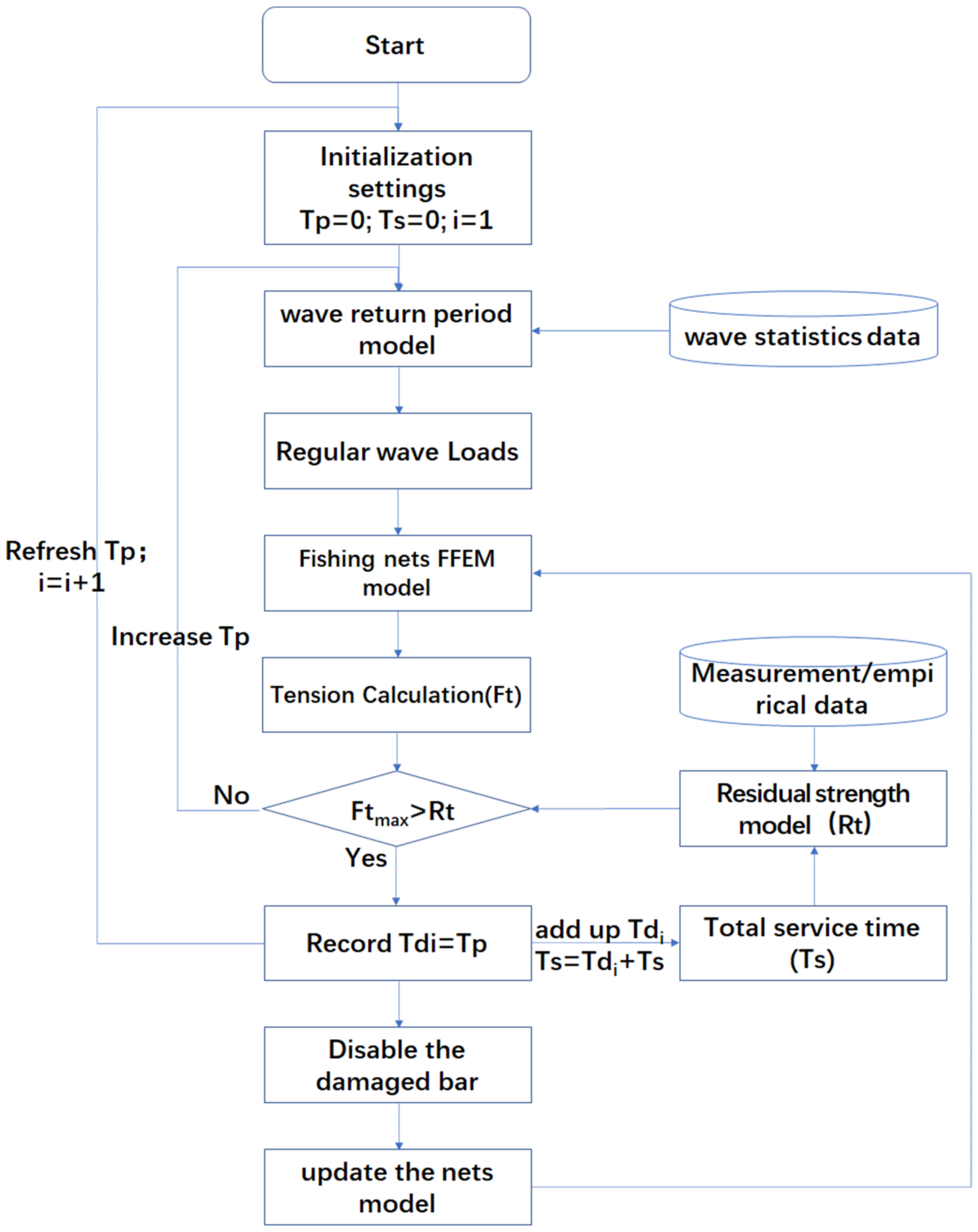
2.1. Basic Workflow of The Dynamic Lifetime Calculation

As shown in Figure 1, the basic workflow of the dynamic lifetime calculation is as follows:

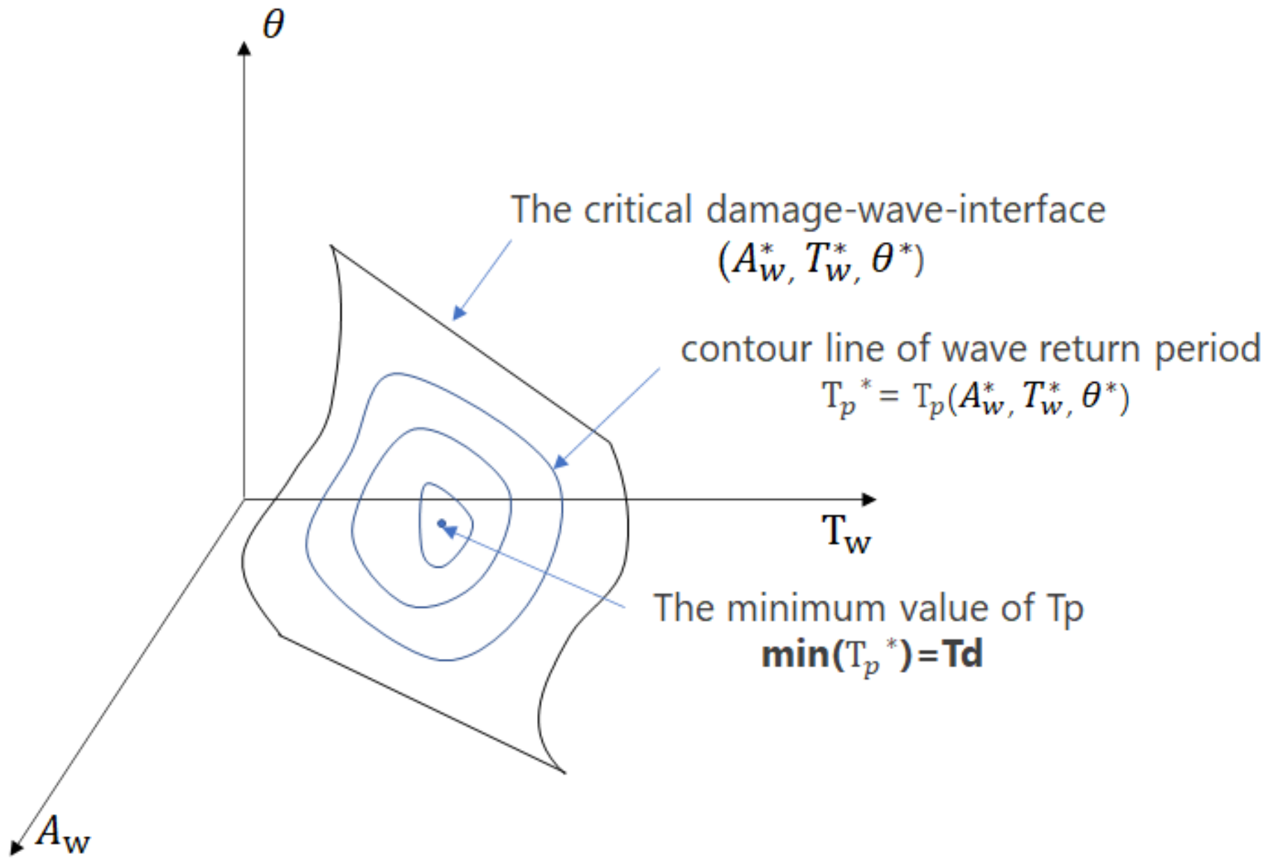
• Step 1: The wave return period model is obtained from the wave statistics data by integrating the wave probability density function (described in detail in Section 2.2). Then, the relationship between the wave load level and the wave return period (Tp) is established.
• Step 2: By applying the Flexible Finite Element Method (described in detail in Section 2.3), the tension (F_T) distribution of the fishing net is analyzed under the wave loads; the tension is determined by the increasing wave return period (Tp) and the corresponding wave load level.
• Step 3: The residual strength model of the netting twine is estimated by fitting the actual measured tensile strength data with an exponential function (described in detail in Section 2.4), through which the tensile strength (R_t) can be calculated under the different expected total service times (Ts).
• Step 4: To determine whether the fishing net is damaged, the maximum tension is compared with the residual strength. The netting twine is judged as damaged if the maximum tension value exceeds the residual strength. The corresponding wave return period is set as the first dynamic lifetime Td₁, and then the dynamic lifetime Td₁ is added to the total service time (Ts).
• Step 5: To rebuild the fishing net model, the damaged twines are set as disabled and removed from the calculation model.
• Step 6: The dynamic lifetime Td_i is calculated by repeating steps 2–5.

Figure 1. The basic workflow of dynamic lifetime calculation (Tp: wave return period since last damage; Ts: total service time of the fishing net; i: current damage sequence number; Tdi: dynamic lifetime of the ith netting twine breaking).

Figure 1. The basic workflow of dynamic lifetime calculation (Tp: wave return period since last damage; Ts: total service time of the fishing net; i: current damage sequence number; Tdi: dynamic lifetime of the ith netting twine breaking).

2.2. Wave Return Period Model

Whether the fishing net will be damaged by a wave load depends on the level of the wave loads during the service time. During a certain time interval, each level of wave shows a different probability of appearance. Generally speaking, the greater the wave amplitude, the lower the chance of that wave’s appearance. To directly correlate the service time with the wave grade, it is necessary to use the wave return period model—the average time interval, called the wave return period $Tp$, in which a wave with a specific characteristic parameter appears twice. At a certain definite sea location and assurance probability, the $Tp$ corresponding to a specific wave is determined statistically.

It is assumed that the wave characteristic parameter $\chi$ follows the two-dimensional probability density function $f\left(\chi ,t\right)$, which can be obtained statistically. To ensure that a wave with a characteristic parameter of $\chi >\chi$^* occurs once under the probability $P$, the wave return period $Tp$ should meet the following probability integral:

$$P^{*}={{\displaystyle \int }}_{X^{*}}^{\propto }{{\displaystyle \int }}_0^{Tp}f(\chi ,t)d\chi dt$$

(1)

Different wave theories obtain different results when given specific characteristic parameters. Miao [11] et al. used an Airy linear regular wave and a Stokes second-order wave, respectively, to simulate the horizontal force of a plane net. A comparison between the calculation and test results shows that the peak error calculated by linear wave theory is 14–23%, and the second-order wave theory has an error range from 7% to 19%. Therefore, the Airy linear wave is selected as the wave to simplify the calculation without a significant loss of accuracy. The velocity potential of the incident wave is:

$$\varnothing =-\frac{ig{A}_w\cosh \left[k\left(Z+h\right)\right]}{\omega \cosh \left(kd\right)}{e}^{i\left[-\omega t+k\left(Xcos\theta +Ysin\theta \right)+\alpha \right]}$$

(2)

where $\varnothing$ is the velocity potential of the incident wave; X, Y, and Z coordinate the microelement position in the overall coordinate system; i is the imaginary unit; $A_w$ is the amplitude of regular waves; g is the acceleration of gravity; ω, k, and h are the wave circle frequency, wave number, and water depth; θ indicates the wave direction angle; and α is the initial phase angle. The fluid particle velocity at a point in space is as follows:

$$\begin{gathered} v=\left(v_x,v_{y,}{v}_z\right) \\ =-\frac{A_w\omega \cosh \left[k\left(z+d\right)\right]}{\sinh \left(kd\right)}{e}^{i\left[-\omega t+k\left(Xcos\theta +Ysin\theta \right)+\alpha \right]}\left(cos\theta ,sin\theta ,-itanh\left\{k\left[z+h\right]\right\}\right) \end{gathered}$$

(3)

where $v_x,v_y,v_z$ are the fluid mass velocity components in three directions. The meanings of the other parameters are the same as mentioned above.

2.3. Flexible Finite Element Method (FFEM)

The two main simplified models for calculating the hydrodynamic force of the netting are the Morison model and the Screen model [17]. The Screen model is applicable to the resistance calculation of the netting, and the Morison model is for a broader range of situations and can calculate the tension distribution of the netting. In this paper, the Morison model is used to calculate the hydrodynamic force of the netting bars.

Because the netting bar is flexible and only bears tensile force, the mass-spring element based on the Morison model has been used to model the netting bars in many previous studies [10]. In this paper, the RIFLEX program, a DNV commercial finite element calculation software is used to perform an analysis of the fishing nets. RIFLEX is a software program that specializes in analyzing flexible offshore riser systems and other slender structures. The Flexible Finite Element Method (FFEM) is used for the calculation of the netting’s tension. The primary techniques for the FFEM of the fishing net are introduced below [18].

2.3.1. Numerical Model Assumptions

In numerical modeling, the following assumptions are made:

• A fishing net is composed of several identical netting bars. Each netting bar is regarded as a cylinder.
• Every netting twine is built as a spatial beam-type line with two end super-nodes.
• Since the number of finite elements of the beam-type line has no influence on the convergence, each line is composed of only one finite element.
• The netting bars are entirely flexible and soft, having only tensile stiffness, which can be realized by setting minimal values to replace the compression, shear modulus, and bending stiffness in the calculation.
• Each bar is connected by nodes that can rotate freely without resistance. Each node has three translational degrees of freedom.
• The mutual interference of the flow field between bars is not considered.

2.3.2. Force Analysis

The forces on a bar element include: gravity $F_W$, buoyancy force $F_B$, hydrodynamics load force $F_D$, and the tension forces $F_T$ applied by adjacent elements. The following Equations (4) and (5) give the gravity $F_W$ and the buoyancy force $F_B$ on a microelement of length dx:

$$d{F}_w={\rho }_0{A}_{s}gdx.$$

(4)

$$d{F}_B=\rho A_{s}gdx;$$

(5)

where ${\rho }_0$ and $A_s$ are the mass density and cross-sectional area of the netting bar, ρ is the mass density of seawater, and $g$ is the gravitational acceleration. The tension $F_{Ti}$ from element $i$ can be written in this form:

$$F_{Ti}=E_m{A}_s\frac{l_i-l}{l}$$

(6)

where $l_i$=$\sqrt{{(X_{i1}-X_{i2})}^2+{(Y_{i1}-Y_{i2})}^2+{(Z_{i1}-Z_{i2})}^2}$ is the length of element $i$ after deformation; $X_{i1},X_{i2},Y_{i1},Y_{i2},Z_{i1},Z_{i2}$ are the deformed location coordinates of the two end nodes of element i; and $E_m, A_{\mathrm{s}}$, and l are the elastic modulus, cross-sectional area, and initial length of netting bars, respectively.

According to Morison Equation, the hydrodynamic load force $F_D$ of a moving object can be written as:

$$F_D=\left(\rho \forall +m_a\right)\dot{V}-m_a\ddot{r}+\frac{1}{2}\rho C_d{A}_c\left|V-\dot{r}\right|\left(V-\dot{r}\right)$$

(7)

where ∀ is the displacement volume; $m_a$ is the added mass and given by $K_M\rho \forall ; K_M$ is the added mass coefficient; $r$ is the translational structural displacement; $C_d$ is the drag coefficient; V is the water velocity; and $A_c$ is the characteristic area.

The motion and the water velocity are broken down into three components in the local element coordinate system, with x in the axial direction and y and z normal to the axis. The hydrodynamic load force’s longitudinal components $F_D^x$ and transverse force components $F_D^y$ and $F_D^z$ on length dx can then be written as:

$$\{\begin{array}{c}d{F}_D^x=dx\left[\left(\rho A_s+m_a^x\right){\dot{V}}_x-m_a^x{\ddot{r}}_x+\frac{1}{2}\rho C_d^x{A}_c^x\left|V_x-\dot{r_x}\right|\left(V_x-\dot{r_x}\right)\right]\\ d{F}_D^y=dy\left[\left(\rho A_s+m_a^y\right){\dot{V}}_y-m_a^y{\ddot{r}}_y+\frac{1}{2}\rho C_d^y{A}_c^y\left|V_y-\dot{r_y}\right|\left(V_y-\dot{r_y}\right)\right]\\ d{F}_D^z=dz\left[\left(\rho A_s+m_a^z\right){\dot{V}}_z-m_a^z{\ddot{r}}_z+\frac{1}{2}\rho C_d^z{A}_c^z\left|V_z-\dot{r_z}\right|\left(V_z-{\dot{r}}_z\right)\right]\end{array}$$

(8)

The calculation parameters in the above formula are as follows:

(1)

For an ideal smooth cylinder, the added mass coefficient in the normal direction is 1, or 0 in the axial direction, that is, $m_{a }^x$ = 0, $m_a^y$ = $m_a^z=$ρ∀.

(2)

$A_c^x$ is the characteristic area in the axial direction, and $A_c^x=\pi dl. A_c^y,A_c^z$ is the component in the normal direction, and $A_c^y=A_c^z=dl.$ $d,l$ are the diameter and length of the netting bars, respectively.

(3)

The flow force coefficient C_D refers to the formula given by Blevins [19] in the Applied Fluid Dynamics Handbook, $C_d^x=0.048, C_d^y$ = $C_d^z=1.2$.

2.3.3. Dynamic Equilibrium Equations

The virtual work equation is used to express equilibrium during the static process. By using Green strains and Piola–Kirchhoff stresses, this equilibrium equation is obtained as:

$${{\displaystyle \int }}_{V_0}^{}\mathit{S}:\delta \mathit{E}d{V}_0={{\displaystyle \int }}_{A_0}^{}{T}_0·\delta \mathit{u}d{A}_0+{{\displaystyle \int }}_{V_0}^{}{F}_0·\delta \mathit{u}d{V}_0$$

(9)

where $\delta$ indicates virtual quantities; $\mathit{S}$ is the Piola–Kirchhoff stress tensor; E is the Green strain tensor; $A_0$ and $V_0$ express the surface and volume of the initial configuration; and $\mathit{u}$ is the displacement vector The surface forces $T_0$ and body forces $F_0$ are referred to as the unit surface and the unit volume in the initial reference state. $\mathit{T}$ includes the hydrodynamic load force $F_d$ and the tension by adjacent element $F_T$; $F_0$ denotes the gravity $F_W$ and the buoyancy $F_B.$ An incremental form of the virtual work principle can be given by:

$${{\displaystyle \int }}_{V_0}^{}\left(\mathit{S}:\delta \Delta \mathit{E}+\Delta \mathit{S}:\delta \mathit{E}\right)d{V}_0={{\displaystyle \int }}_{A_0}^{}\Delta {\mathit{T}}_0·\delta \mathit{u}d{A}_0+{{\displaystyle \int }}_{V_0}^{}\Delta {\mathit{F}}_0·\delta \mathit{u}d{V}_0$$

(10)

where $\Delta$ is used to denote the increment between two neighboring equilibrium configurations. During the dynamic process, the dynamic equilibrium equation expressed in terms of virtual work is formulated as follows:

$${{\displaystyle \int }}_{V_0}^{}\mathit{S}:\delta \mathit{E}d{V}_0+{{\displaystyle \int }}_{V_0}^{}{\rho }_0\ddot{\mathit{u}}·\delta \mathit{u}d{V}_0+{{\displaystyle \int }}_{V_0}^{}\tilde{c}\dot{\mathit{u}}·\delta \mathit{u}d{V}_0={{\displaystyle \int }}_{A_0}^{}{T}_0·\delta \mathit{u}d{A}_0+{{\displaystyle \int }}_{V_0}^{}{F}_0·\delta \mathit{u}d{V}_0$$

(11)

where ${\rho }_0$ denotes the mass density of the netting bars, and $\tilde{c}$ is the viscous damping density function. Compared to Equation (9), the two additional terms appearing in Equation (11) stem from the inertia forces and the damping forces. The incremental form of Equation (11) equates to:

$$\begin{array}{c}\hspace{1em}\hspace{1em}\hspace{1em}{{\displaystyle \int }}_{V_0}^{}(\mathit{S}:\delta \Delta \mathit{E}+\Delta \mathit{S}:\delta \mathit{E})d{V}_0+{{\displaystyle \int }}_{V_0}^{}{\rho }_0\Delta \ddot{\mathit{u}}·\delta \mathit{u}d{V}_0+{{\displaystyle \int }}_{V_0}^{}\tilde{c}\Delta \dot{\mathit{u}}·\delta \mathit{u}d{V}_0\\ ={{\displaystyle \int }}_{A_0}^{}\Delta {\mathit{T}}_0·\delta \mathit{u}d{A}_0+{{\displaystyle \int }}_{V_0}^{}\Delta {\mathit{F}}_0·\delta \mathit{u}d{V}_0\end{array}$$

(12)

2.3.4. Equation Solving Method

Equation (12) shows a group of nonlinear second-order differential equations, which cannot obtain accurate analytical solutions and need to be solved by numerical approaches. Spatial discretization and time difference are the primary ways to solve continuous differential equations. The linearized time-domain equations are solved in the discrete space, and the static equilibrium equations are solved in each time step.

After the spatial discretization, Equation (12) can be written in the following linearized standard form:

$$M\ddot{r}+C\dot{r}+Kr=R^E\left(r,\dot{r},t\right)$$

(13)

where,$M,C, \mathrm{and} K$ are the tangential mass, damping, and stiffness matrices evaluated at the static equilibrium position, and r is the dynamic displacement vector relative to the static position. RE is the dynamic load vector expressing the difference between the total external load vector and the external load vector at static equilibrium. These equations are solved by the NEWMARK-β method.

A static finite element analysis is performed in each time step, and Equation (13) can be expressed as a time-independent equilibrium form:

$$R^S\left(r\right)=R^E\left(r\right)$$

(14)

where $R^S\left(r\right)$ and $R^E\left(r\right)$ indicate the internal structural reaction vector and the external force found by the assembly of element contributions. The equation is solved by an equilibrium iteration using the Newton–Raphson method.

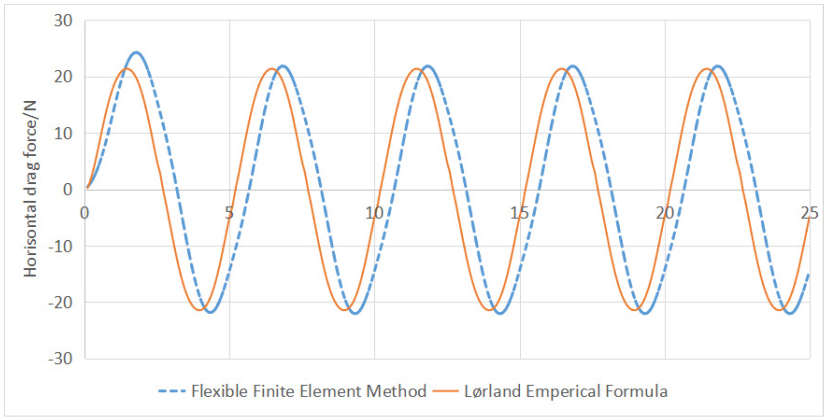
2.3.5. Checking the Force Calculation Result by Løland’s Empirical Formula

Lørland [20] put forward an empirical formula for calculating the net’s drag and lift force based on the screen model method. The horizontal resistance force of the square mesh netting is calculated by the empirical formula to check the reliability of the force calculation by the FFEM in this paper. The formulas for the drag coefficient $C_N$ and the lift coefficient $C_L$ of the square mesh netting are as follows:

$$\left\{\begin{array}{c}{C}_N=(0.04+-0.04+0.33S_n+6.54S_n^2-4.88S_n^3)\mathrm{c}\mathrm{o}\mathrm{s}\mathsf{\phi }\\ C_L=-0.05S_n+2.3S_n^2-1.76S_n^3\sin \left(2\mathsf{\phi }\right)\end{array}\right.$$

(15)

where $S_n$ is the netting’s solidity ratio, and $S_n=2\frac{d}{l}-{\left(\frac{d}{l}\right)}^2.$ d and l are the diameter and length of the netting bars, respectively; and $\mathsf{\phi }$ is the angle between the normal direction of the netting and the water flow direction. It should be noted that these formulas only apply to square mesh netting (the opening angle of the mesh is 90°). A comparison of the horizontal resistance force calculated two ways is discussed in Section 3.2.

2.4. Residual Strength Model and Breaking Criterion

Netting twine is usually made of polymer fibers. Compared with metal materials, the breaking conditions of netting twine are more complex. The tensile strength of polymer materials is affected by many factors, such as natural aging, dynamic fatigue, static fatigue (creep), abrasion, and many other factors. In addition, the mechanical properties are very different in different media, such as seawater or air. Although different property tests can be carried out on the netting twine material individually or jointly to obtain the breaking conditions in a laboratory setting, it is still challenging to predict the tensile strength under actual service conditions due to the coupling effect of various factors and the limitations of experimental conditions.

At present, classical fishing gear mechanics [3,21] generally use the residual strength model to describe a fishing net’s strength performance. The empirical formula of the residual strength is obtained through the actual measurement of the netting twine’s strength after a certain period of service. Based on the intuitive understanding that “the strength will decrease more and more rapidly with the service time increasing”, it is assumed that the strength of the fishing net will decrease exponentially with the service time. The residual strength formula of the netting twine may be written as:

R_t = a R₀ (L − t)^b + R_L;

(16)

where R_t is the residual strength after t service time, R₀ is the initial tensile strength, R_L is the residual strength after L service time, and a and b are the parameters comprehensively reflecting the material ability and work conditions. The formula directly reflects the change in material strength with the service time and avoids resolving the influence of complex factors on the strength. The residual strength model was mainly used to evaluate the life of net-ropes, but it has not been used to predict the damage lifetime of netting. It provides a practical way to predict the fishing nets’ lifetime.

For different structure forms, sea locations, and maintenance conditions, the main factors leading to the rupture of fishing nets may be different. However, the problem becomes complex and challenging if all aspects are considered separately. As far as large-scale aquaculture net cages that are well-maintained and located in open marine areas are concerned, the hydrodynamic wave force is the main factor in the fishing nets’ breakage. Therefore, the residual strength is used as the criterion for the judgment of breakage, and the specific influence of other factors is ignored or considered in the residual strength model. The judgment criterion for a fishing net’s breakage under a wave load is set as follows:

F_Tmax = R_t

(17)

where F_Tmax is the maximum tension value of the netting twine under the wave load, which is obtained through the FFEM simulation calculation, and R_t is the residual strength of the net’s twine at the service time t, given by Equation (16).

3. Results and Discussion

The method proposed and presented in the previous section is applied to calculate the case model described in Section 3.1. The horizontal resistance calculated by the RIFLEX software is compared with the empirical formula in Section 3.2, which can help verify the results. Section 3.3 presents the netting’s tension calculation result and discusses the tension distribution rule and the dangerous area. The effects of the wave’s characteristic parameters on the tension of the netting are discussed in Section 3.4. Section 3.5 predicts the development path of the damage and the maximum change in tension trends during the breaking process. The two nettings’ dynamic lifetime prediction results are introduced in Section 3.6.

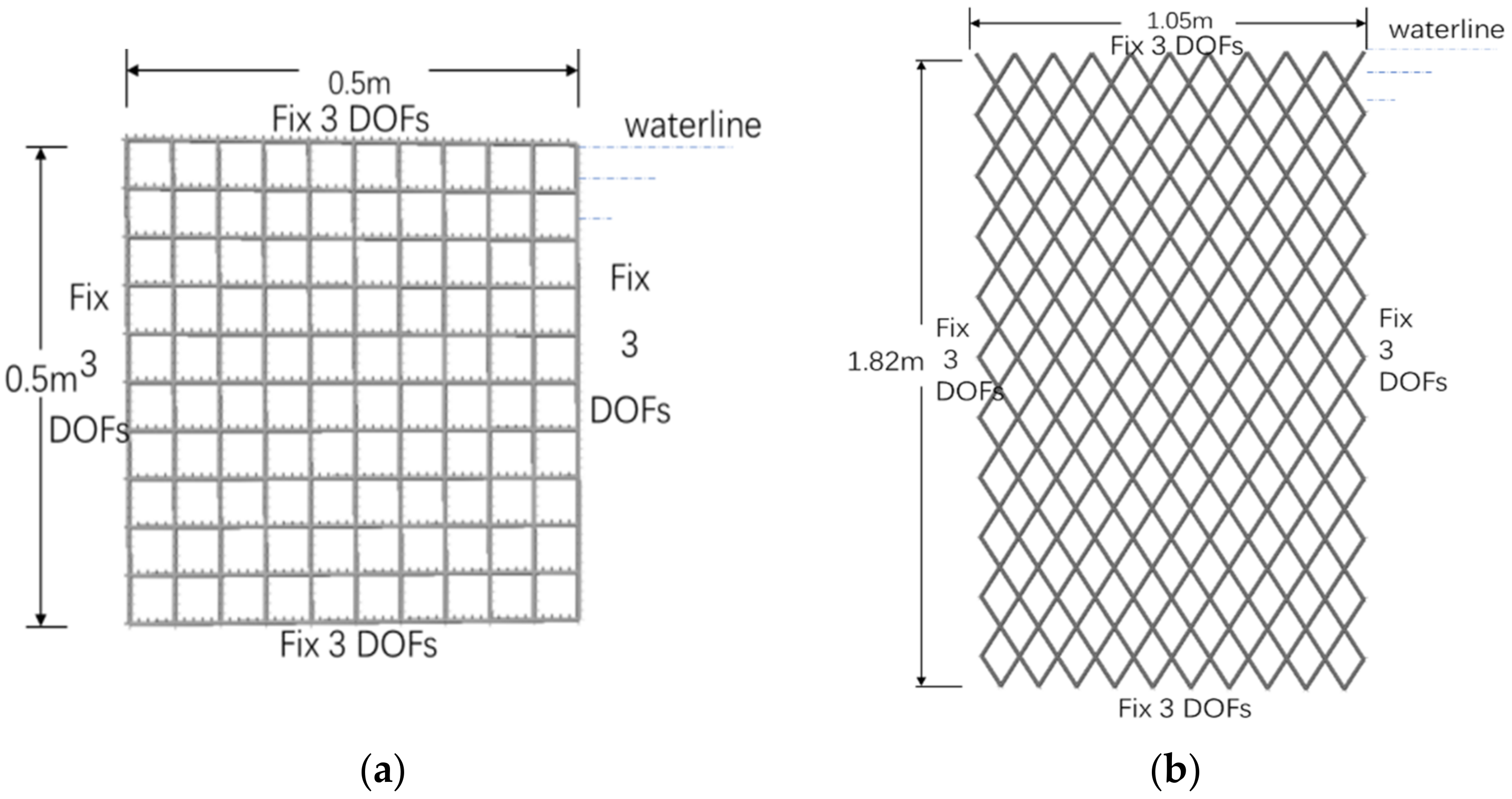
3.1. Calculation Model

Two types netting, a square and a diamond mesh, were selected for the case study. Both nets are knotless and comprised of ten lines of mesh in the transverse direction (T-direction) and ten in the vertical direction (N-direction). To simulate the tensioned netting’s boundary conditions, the translation and rotation degrees of freedom of the nodes on the four edges of the netting are set to fixed and free, respectively. The model’s twine diameter, bar length, material density, axial stiffness, and coefficient of knot shrinkage for calculation come from the specific physical netting. However, to reduce the calculation scale, the selected netting size is smaller than the actual one. The netting model is shown in Figure 2, and the basic model parameters are given in

Table 1. Basic parameters of the netting model.

Mesh Type	Twine Diameter	Bar Size	Material Density	Axial Stiffness	Coefficient of Knot Shrinkage	Netting Size	Number of Elements
	m	m	kg/m3	N/m		m
Square	3.8 × 10−3	0.05	917.5	1.69 × 106	$\begin{array}{c}{E}_n=0.707\\ E_t=0.707\end{array}$	0.5 × 0.5	220
Diamond	7.6 × 10−3	0.1	917.5	3.37 × 106	$\begin{array}{c}{E}_n=0.5\\ E_t=0.866\end{array}$	1.05 × 1.82	452

.

Many scholars have conducted simulation calculations for trawls, purse seines, gravity nets, etc., but there are few calculations for four-sided tensioned fishing nets used for deep-sea cages. Therefore, it is of practical value to select this model for calculation.

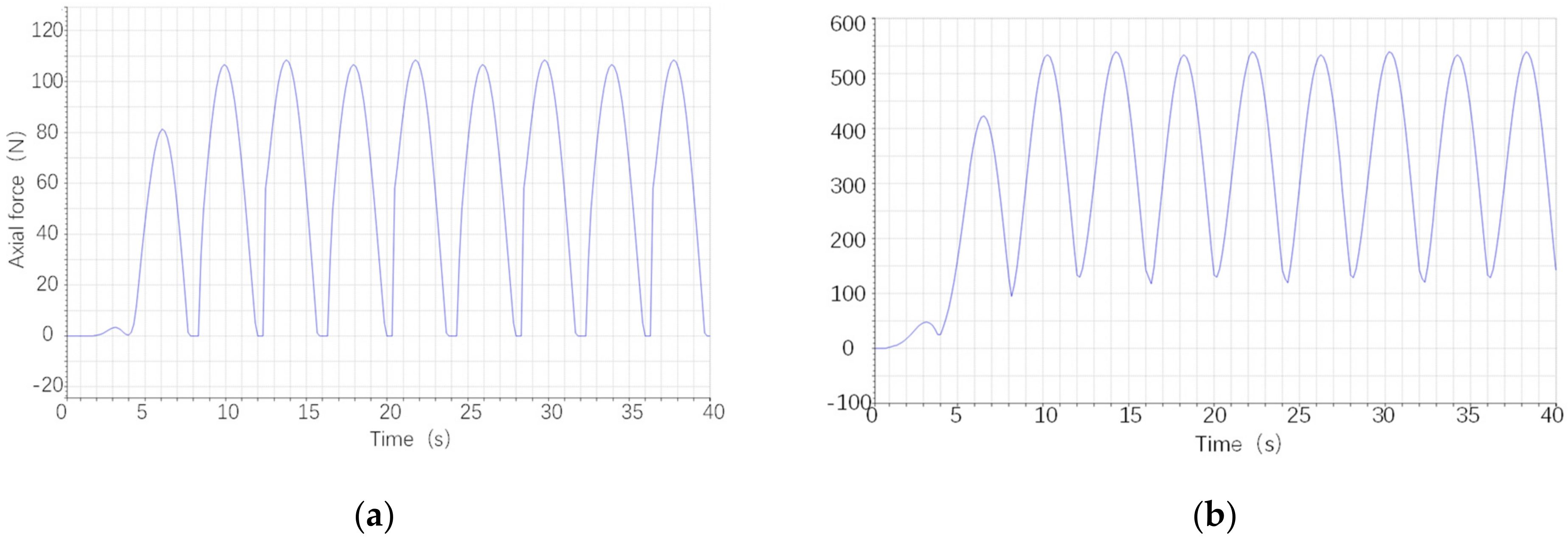
3.2. Checking the Force Calculation Result

The horizontal drag force of the square mesh netting calculated by the FFEM and the empirical formula is shown in Figure 3:

In Figure 3, it can be seen that the peak values of the netting’s horizontal drag force calculated by the FFEM are very close to that of the empirical formula. The difference is tiny, because the selected hydrodynamic parameters in the FFEM calculation come from the classic experimental data, which comply with the Lørland empirical formula. Although there is some difference in the phase angle, it does not influence the result of the netting’s lifetime.

Because the horizontal drag force calculated by the FFEM is the sum of the horizontal components of the tension of all netting bars connected to the frame, the comparison results can prove the reliability of the netting tension calculation in this paper.

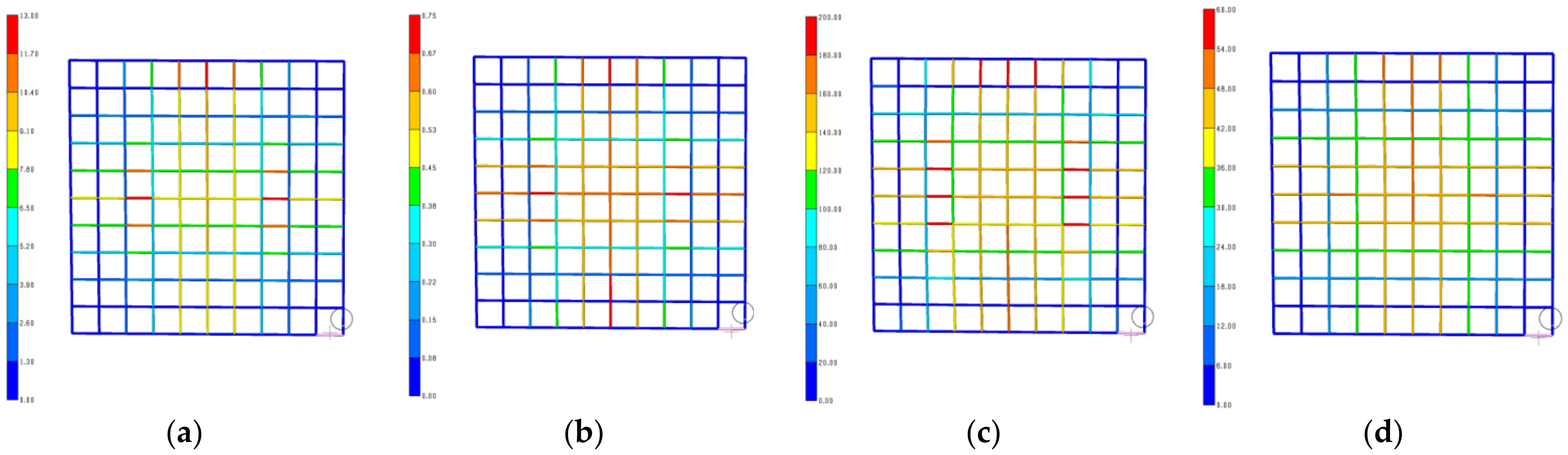
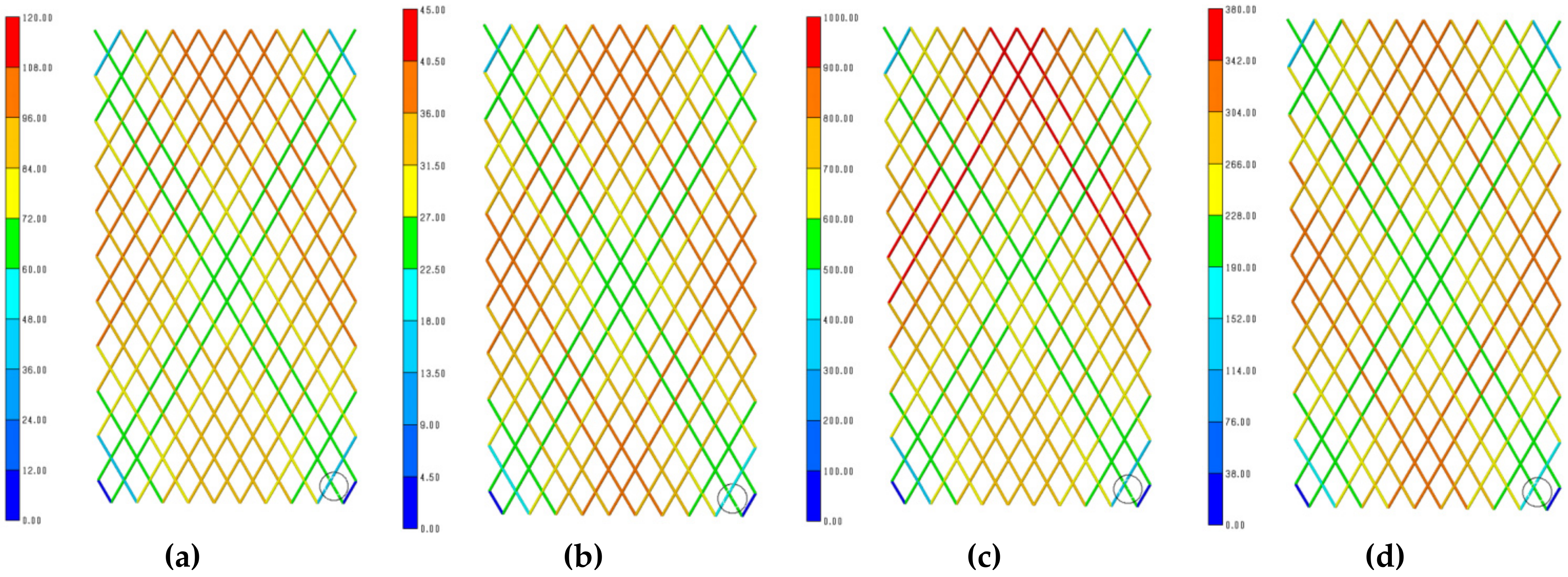
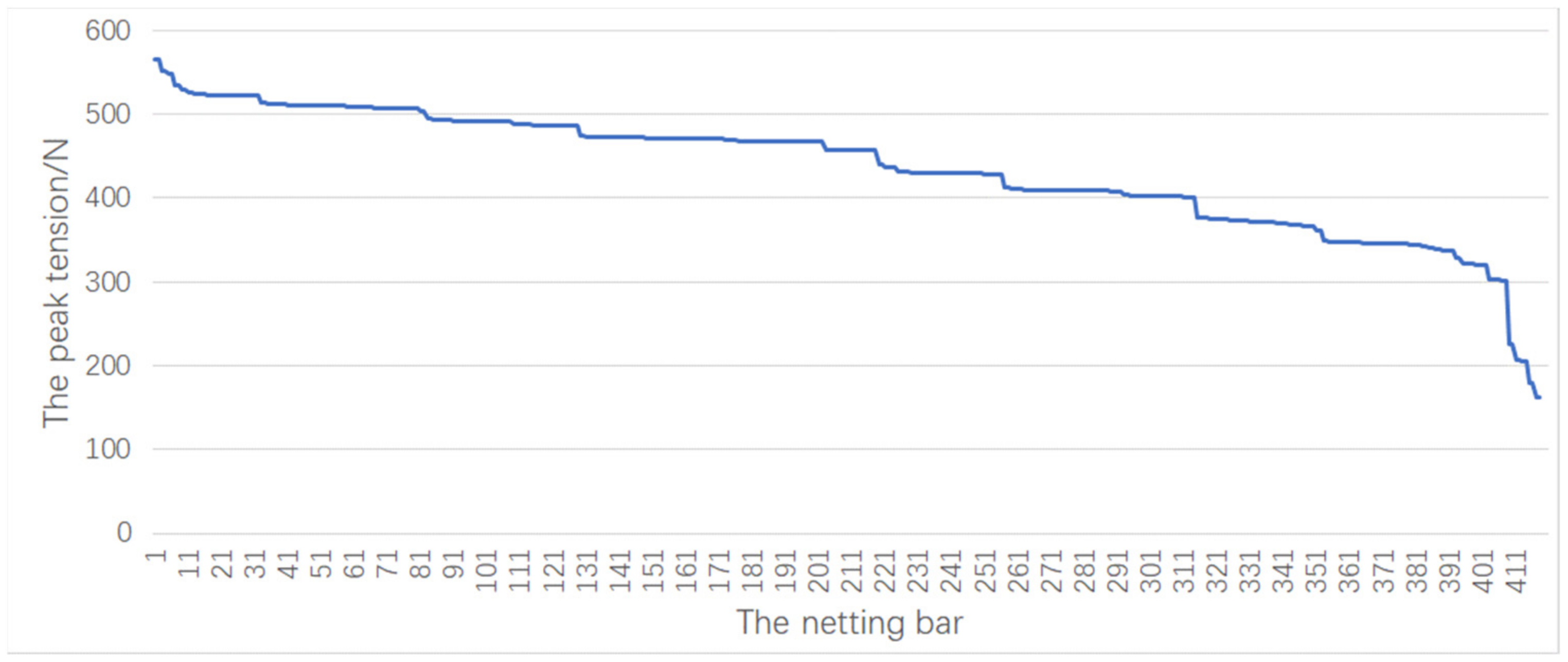
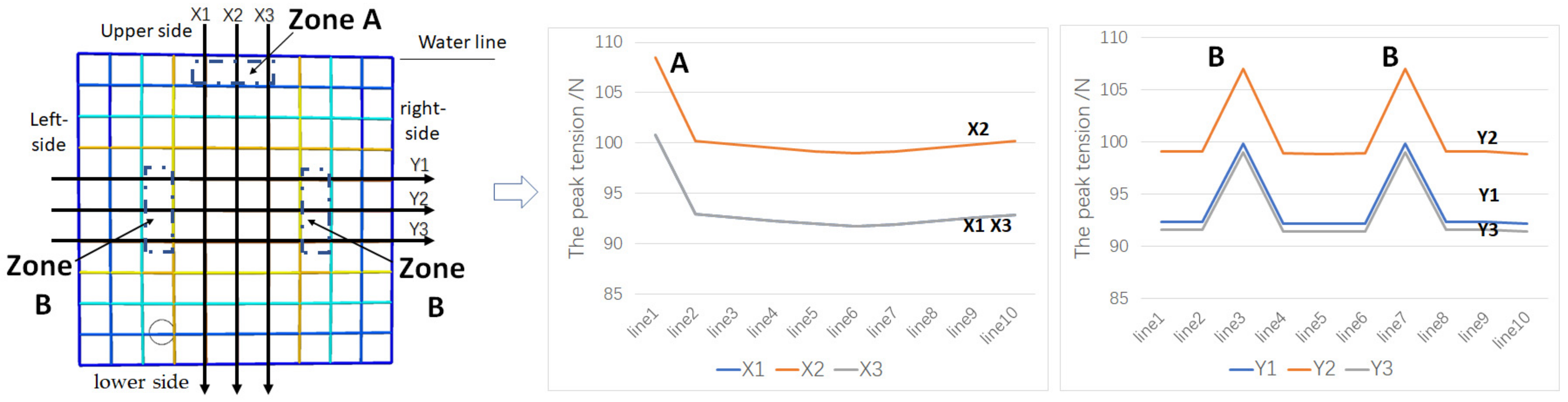
3.3. Determination of Hotspot Areas

Some authors have studied the tension distribution of nets under current loads or the resistance of nets under wave loads, but few have studied the tension distribution of nets under wave loads. It is valuable to observe the peak tension distribution of the fishing net under wave conditions.

Several waves with different amplitudes and periods that come from the observation record in the South China Sea and have a variation range of 1–5 m in wave amplitude and 5–16 s in wave period were chosen to calculate the netting tension. The incident angle of the wave θ is set as 0°. When Aw = 5 m, Tw = 8 s, and θ = 0°, a typical time-domain variation of the netting bar’s tension on the two types of netting is illustrated in Figure 4.

It can be observed in Figure 4 that the tension fluctuates periodically between the valley and the peak value, and the variation period of the tension is half of the wave period. According to the breaking criterion introduced in Section 2.4, only the peak values need to be considered. The peak tension value of each bar is extracted and illustrated in the colored pattern (as shown in Figure 5 and Figure 6).

It can be seen in Figure 5 and Figure 6 that, although the wave amplitude and period are different, the peak tension value of the bars has a similar distribution. The tension hotspots are concentrated at the connection lines of the midpoints of the four edges along the netting bars’ direction. The tension hotspot of the square mesh netting is in the shape of “╬”, and the diamond mesh netting’s hotspot is in the shape of “◇”. The change in wave parameters has no noticeable effect on the relative position of the tension hotspot.

Li [10] et al. calculated the tension of a diamond mesh plane netting in flow load. However, the boundary condition of Li’s netting was that both two were free, the top was fixed, and the bottom weighted, which differs from the case in Figure 2b. The tension distribution in the middle part of the fishing net in Li ‘s case is similar to the case for calculation in Figure 6. The calculation results in this paper show the tension distribution of four-sided fixed fishing nets under wave loads, which is close to the actual situation of a deep-sea aquaculture cage fishing net. Through comparison, it can be found that there is always a stress hotspot at the midpoint of the fixed edge of the fishing net, whether it is because of a wave or a current load.

The peak tension values of all bars are illustrated in sequence from the largest to the smallest value in Figure 7 and Figure 8.

It can be observed in Figure 7 and Figure 8 that:

• The peak tension value of the bars follows a ladder distribution. Compared with the diamond mesh netting, the tension distribution of the square mesh netting is steeper.
• In the square mesh netting, the peak tension of nearly half the bars is less than the median value of the maximum tension of the netting. However, most of the bars in the diamond mesh netting have a peak tension exceeding the median value of the maximum tension of the netting.

This result may imply that the material utilization rate of the diamond mesh netting is higher than that of the square mesh netting, but this still needs additional study to be definitely proven.

To further study the tension hotspots, the distribution of the peak tension value of each column of netting twine near the tension hotspots is illustrated in Figure 9 and Figure 10.

For the square mesh netting, the maximum tension area appears at the vertical netting bars near the midpoint of the upper boundary side (as shown in Figure 9, zone A). The second-largest tension area appears at the transversal netting bars near the two quartile positions of the midpoint line both on the left and right side (as shown in Figure 10, zone B). The bar’s tension in zone A is slightly greater than that in zone B.

For the diamond mesh netting, the maximum tension appears at the netting bars near the midpoint of the upper boundary side (as shown in Figure 10, zone C). The second-largest tension areas appear at the midpoint of the left or right boundary sides (as shown in Figure 10, zone D). The bar’s tension in zone C is significantly greater than in zone D.

The above tension distribution characteristics of the two types of nets can be similarly observed under other wave parameters. According to the breaking criteria, the results above indicate that the netting bars in zone A or C are the most prone to be damaged, closely followed by zone B or D, and finally, the other netting bars in the high-tension regions (i.e., “╬”or “◇” area). This feature is particularly obvious in the diamond mesh nettings.

The author obtained some photos as a comparison reference that shows the actual damage in zone C and zone D on the diamond mesh nettings of deep-water gravity cages (as shown in Figure 11b). The extent of the damage to the bars in zone C is significantly worse than in zone D. This proves that the prediction of the damaged position is reliable. Since the boundary condition of deep-water gravity cage nettings is similar to that of tensioned nettings, the real cases in Figure 11b have a good reference value for verifying the calculations.

In order to increase the lifetime of a fishing net, the netting should be especially strengthened near the waterline and middle of the vertical rope. Structural wear, marine organism corrosion, and unnecessary openings in dangerous areas should also be avoided as much as possible.

3.4. Influence of Wave Parameters on the Tension

The maximum tension of the two types of nettings was calculated under different wave amplitudes, periods, and incident angles. The calculation result of the maximum tension of the two types of nettings with different wave parameters is shown in Figure 12.

It can be observed in Figure 12 that all three parameters have an apparent effect on the tension of the netting. The maximum tension on both nettings increases steadily with the wave amplitude and decreases steadily with the wave period and incidence angle. The results also show that the square mesh netting is more significantly affected by the variation in wave parameters than the diamond mesh netting. However, ascertaining whether the mesh type or other factors lead to this sensitivity difference needs further study.

These results can be explained well by Equation (3). With the increase in wave amplitude or the decrease in wave period, the water velocity increases correspondingly, leading to increased hydrodynamic loads on the nettings. When the wave incidence angle increases, the velocity component in the normal direction of the netting will decrease, too, as the water velocity in the normal direction plays the main role in causing the deformation of the netting.

Generally, an aquaculture cage is installed and works in a certain sea area and will not change locations during its lifetime. Although the angle at which the wave amplitude, period, and direction will appear is determined and basically stable, the relative wave incidence angle may be changed by proper installation approaches to reduce the maximum tension of the nets. Figure 13 shows suggestions for the installation modes of two polygon cages. By adjusting the direction of the cages, the maximum tension of the nets of the rectangular cages can be reduced by 13–35%, as well as by 4–15% for the hexagonal cages. By rotating the cage’s direction regularly every year so that the netting in different areas can take turns bearing the wave force, there is a chance to significantly improve the lifetime of the fishing net.

According to the monotone features of the wave parameters’ effect on the tension, the wave space can be easily divided into two continuums of spaces: the damaged wave space under whose loads the netting will be damaged, and the undamaged wave space under whose loads the netting will not be damaged. The tension of the netting bars under the wave parameters ($A_w^{*}$_, $T_w^{*}$_, ${\theta }^{*}$) in the critical damage-wave-interface between the two wave spaces causes the breakage to the nettings. The minimum return period of the waves, min ($T_p{}^{*}$), in the critical damage-wave-interface, corresponds the lifetime (Td) of the netting. The relationship between the critical damage-wave-interface and the lifetime of the netting is shown in Figure 14.

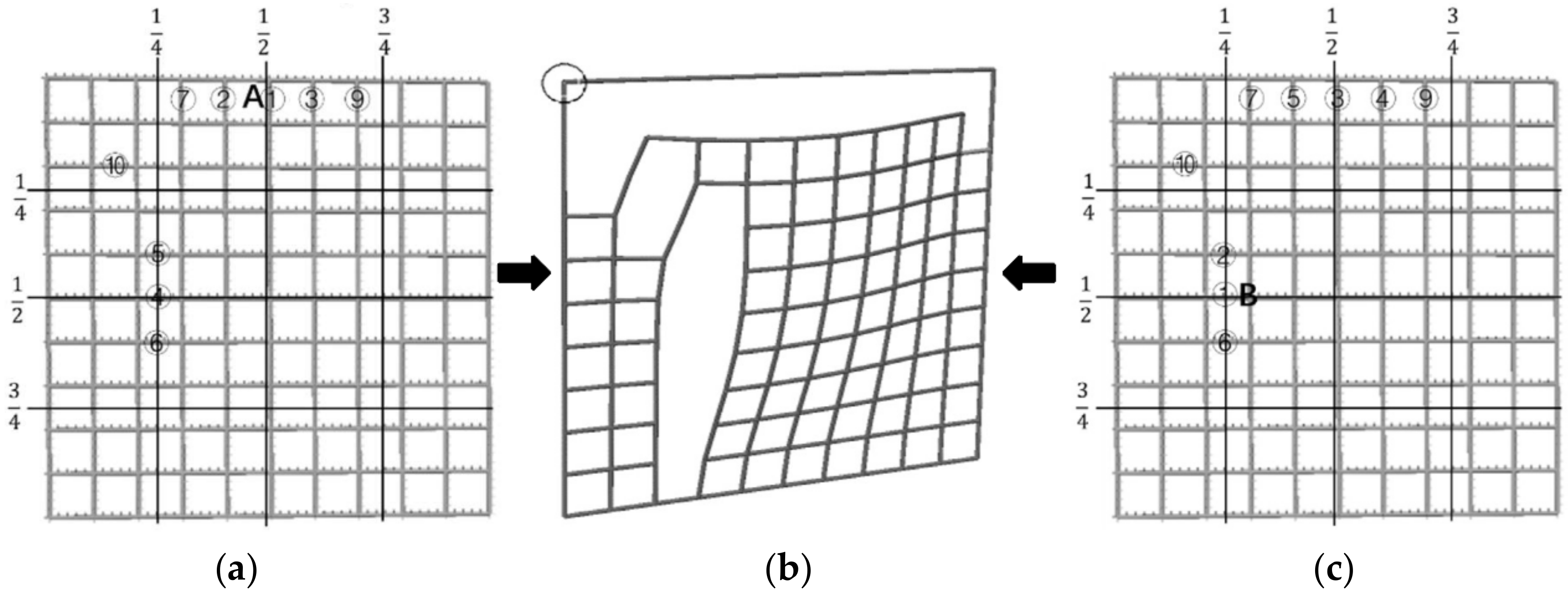
3.5. Prediction of Damage Development in the Netting

According to the breakage criterion, the netting bar with the maximum tension is the most likely to be broken. Once damage occurs, the distribution of the netting’s tension will be redistributed to the remaining bars, so it is necessary to re-calculate the tension in the remaining bars and determine which bar has the highest chance of rupturing next.

Section 3.3 shows that the bars in zones A, B, C, and D are significantly more likely to be damaged than those in other areas. Therefore, zones A and B are respectively selected as the assumed initial positions of breakage for the square mesh netting, and zones C and D are selected for the diamond mesh netting. After the initial breakage occurs, the maximum tension will be transferred to another bar, causing its subsequent damage. The damage will develop along two certain paths, one that starts from zone A/C and one that starts from zone B/D. Eventually, the damaged netting will appear in a certain pattern. The maximum tension of the netting will also change dynamically during this damage development process.

Figure 15 shows the path of damage development and the damaged pattern in the square mesh netting, and Figure 16 shows the change in the maximum tension with the increase in the number of broken bars. Figure 17 and Figure 18 show the corresponding results for the diamond mesh netting.

According to Figure 15 and Figure 16, the rule of the damage development process in the square mesh netting can be summarized as follows:

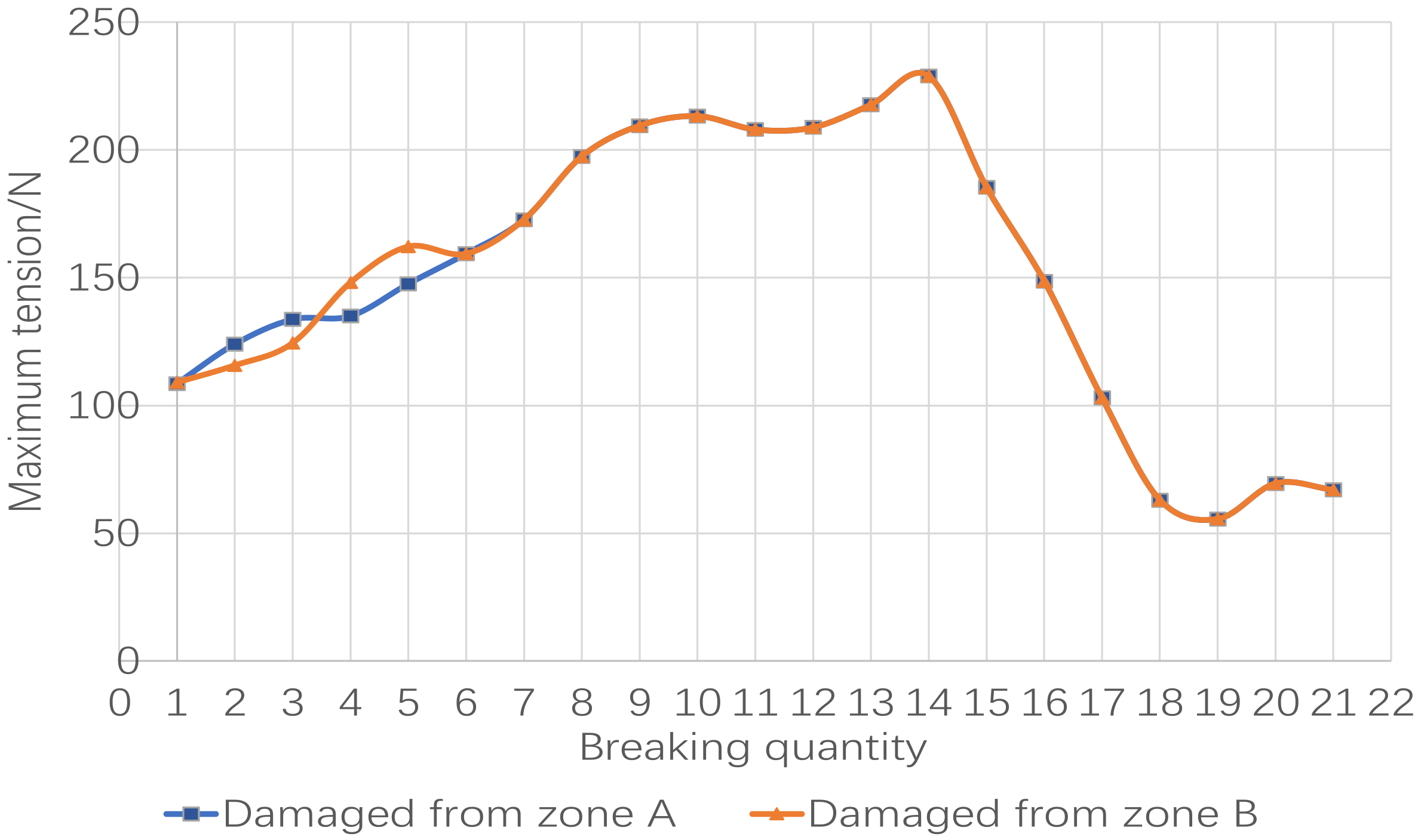
• Whether the square mesh netting is damaged from zone A or B, the netting bars in zone B or A will rupture in the subsequent damage process, and the netting will eventually show the same damaged form.
• The maximum tension changing trends along the two paths of damage development are similar at the beginning stage of the damage process and the same in the subsequent process. The maximum tension will generally increase at the beginning stage of the damage process and decrease rapidly when the destructive area expands to a large enough extent.

The phenomenon of rapid tension dropping in Figure 16 may be explained by the fact that as the damaged area expands, the netting loses so many areas resistant to water flow that the wave hydrodynamic load drops.

The rule of the damage development process of the diamond mesh netting can be summarized as follows from Figure 17 and Figure 18:

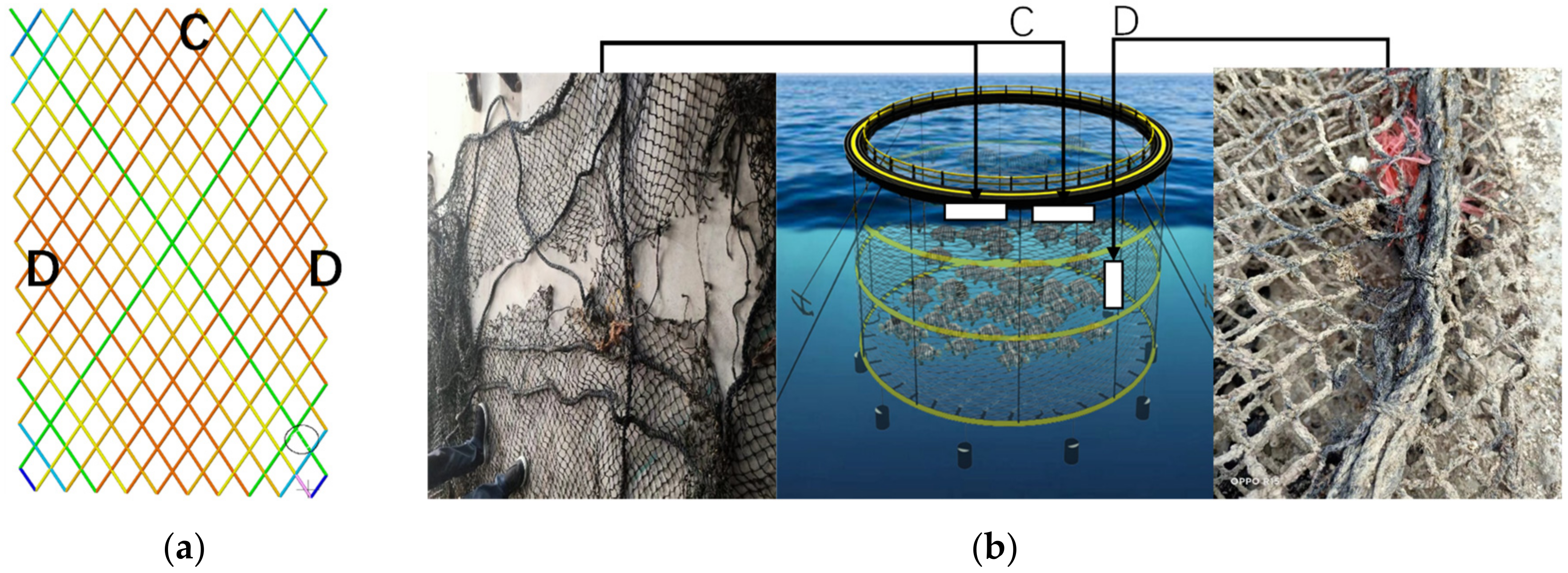
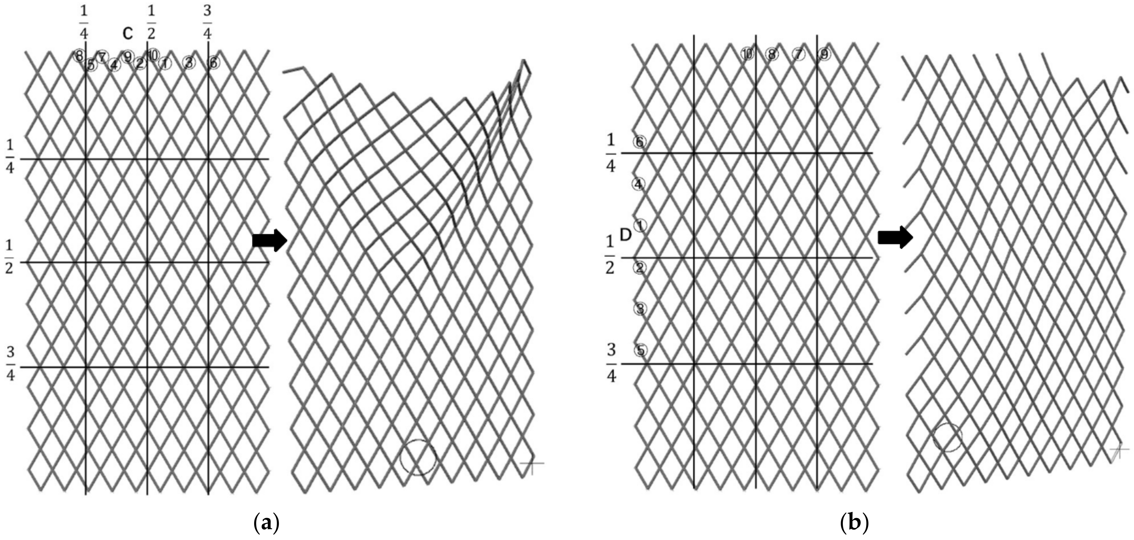
• The diamond mesh netting will result in different damaged forms when damaged from either zone C or zone D. When the damage begins from zone C, the area of the continuous damaged hole is more significant than that from zone D.
• The maximum tension of the diamond mesh netting increases at first and then drops at the beginning stage of the breakage process. When the net is damaged to a certain extent, the maximum tension will increase rapidly in a volatile pattern. The growth rate of the maximum tension from zone C is greater than that of zone D.

The following conclusions may be drawn based on the analysis above: If a fishing net encounters a wave load significant enough to cause initial damage, the damage will constantly expand until the wave loads decrease or the netting is damaged to a large enough extent.

Figure 19 shows a comparison between the predicted damaged form and the real netting damage on a deep-water gravity cage. The prediction of the damaged form coincides with the real case. This can prove the reliability of the damage path prediction and the maximum tension changing trends from our calculation.

3.6. Dynamic Lifetime Prediction of the Netting

Assuming the netting is broken from area A and along the path given in Section 3.5, the dynamic lifetime of the two types of netting is calculated under the given residual strength model and wave return period model.

The initial tensile strength of the square and diamond mesh netting twine is set as 214 N and 856 N according to their twine diameter. Because the model size in the calculation is smaller than actual netting, and the calculated tension is much lower than the tension of real-sized netting, the tensile strength is artificially set lower than that of actual netting twines (such as the UHMWPE twines) with the same diameter. By doing this, the netting tension and the residual strength can be compared at the same level. The residual strength of the netting twine after five years is 10% of its initial strength. The parameters a, k in the residual strength model are 0.343 and 0.6. The residual strength in each year is shown in

Table 2. Residual strength of the netting twines.

Mesh Type	t/year	0	1	2	3	4	5
Square	R(t)/N	214	190	163	133	95	21
Diamond		856	760	653	531	379	86

:

The residual strength of the netting twines under different service lives can be drawn from Figure 20.

To simplify the calculation, only the wave amplitude is regarded as a variable parameter of the wave space. The return period of the waves at a given probability is given in

Table 3. The wave return period varies with the wave amplitude ($T_w=8 \mathrm{s}, \theta =0$).

Wave Amplitude/m	1	2	3	4	5	6	7	8
Return Period/years	0.042	0.067	0.17	0.33	0.5	0.92	1.67	3.75

.

The maximum tension of the nettings is calculated under different service times and the corresponding wave amplitudes according to the model of the wave return period given in

Table 4. Dynamic lifetime calculation results.

Netting	Dynamic Lifetime (Year)
	Td1	Td2	Td3	Td3
Square mesh	1.56	0.79	0.53	0.45
Diamond mesh	1.1	0.58	0.46	0.39

. Figure 21 shows the maximum tension under different service times when the netting is not damaged.

Sharing the same ordinate system, the residual strength curve (as shown in Figure 20) and the maximum tension curve (as shown in Figure 21) are drawn in the same graph. The time at which the maximum tension reaches the residual strength is the first dynamic damage lifetime (Td₁), as shown in Figure 22.

Disabling the first damaged netting twine, taking the first lifetime (Td₁) as the starting point to recalculate the service time, and recalculating the maximum tension curve of the netting under different service times (as in Figure 21), the new tension curve is drawn in Figure 20, and the time at which the maximum tension reaches the residual strength is the second dynamic lifetime (Td₂). The subsequential dynamic lifetimes (Td_i) are obtained by analogy, as shown in Figure 22. The dynamic lifetime calculation result is listed in Table 4.

As shown in

Table 5. Relative dynamic lifetime calculation results.

Netting	Relative Dynamic Lifetime
	Td1/Td1	Td2/Td1	Td3/Td1	Td3/Td1
Square mesh	1	0.51	0.34	0.29
Diamond mesh	1	0.53	0.42	0.35

, the dynamic lifetime of both nettings becomes shorter and shorter with the increase in service time. It is worth noting that this table does not indicate that the lifetime of diamond nets is shorter than that of square nets because the two nets have different sizes. The effect of fishing net types on the lifespan of the fishing net needs to be further studied.

The prediction of the dynamic lifetime of a fishing net can provide a feasible means for an environmental viability assessment of cage site selection. If the estimated lifetime of the fishing net is lower than the design requirements, it is necessary to relocate the cage or implement a safer netting design.

Since the absolute value of the dynamic life is not comparable, the dimensionless relative dynamic lifetime is defined as the dynamic life Td_i divided by Td₁. The relative dynamic lifetime is calculated and shown in Table 5 and Figure 23.

Figure 23 shows that the nets first broken have the most extended dynamic lifetime, and the subsequent dynamic lifetime becomes shorter and shorter. The development of damage to the square mesh is faster than that of the diamond mesh. This may be because the tension distribution of square mesh is more uneven than that of the diamond mesh or because the number of bars in the square mesh netting is less than the number of bars in the diamond mesh netting.

In addition, the relative dynamic lifetime curves of the two types of netting are very close, and the relative lifetime of the second breaking is almost the same. This rule provides a way to predict the time of the subsequent damage according to its initial fracture lifetime. An additional study is needed to unearth which factors mainly determine the relative dynamic lifetime.

However, this method needs to be further studied in a quantitative way. Limited by the production statistics data, the quantitative actual lifetime data do not yet exist to verify the dynamic lifetime prediction of the nettings. Nevertheless, the method and results can explain the accelerated extension of the nets’ damage mentioned above [4].

The practical significance of the relative dynamic lifetime curve for engineering is that it provides a way to infer the next possible time of damage by recording several previous dynamic lifetimes.

4. Conclusions and Future Works

Because it is difficult to obtain an accurately damaged property model of fishing net materials that correspond to the actual service conditions, the classic cumulative damage method based on the S-N curve or crack growth model to predict the lifetime of the fishing net is unrealistic. In this paper, a novel and practical method based on the wave return period model and residual strength model is presented to estimate the dynamic lifetime of fishing nets under different quantities of damaged netting bars. Square and a diamond mesh tensioned plane nettings were selected as the case study models.

The tension distribution rules of the nettings are calculated by the Flexible Finite Element Method (FFEM) under regular wave loads. The horizontal force of the square mesh netting in regular waves calculated by the FFEM has good agreement with the result calculated by the Lørland empirical formula. According to the tension distribution, it is predicted that the damage will most likely appear in the areas near the midpoint of the upper fixing boundary side for both nettings. The damage zone prediction of the diamond mesh netting is verified by real damaged nets. The tension distribution curve of diamond mesh netting is more uniform than the square mesh netting, which implies that the diamond mesh has a higher material utilization rate than that of square mesh. It can be inferred that diamond mesh is more durable than square mesh under the same type and quantity of net materials.

The influence of wave parameters on the netting’s maximum tension was studied. The wave amplitude, wave period, and incidence angle have an apparent effect on the maximum tension of the nettings. The maximum tension on both nettings increases steadily with the wave amplitude and decreases steadily with the wave period and incidence angle. The peak tension of square mesh netting is more significantly affected by the variation in wave parameters than the diamond mesh netting. By adjusting the direction of the cages, the maximum tension of the nets of the rectangular cages can be reduced by 13–35% and by 4–15% for the hexagonal cages. The correct installation direction of the cage can effectively increase the service lifetime of the fishing net.

The paths of damage development, maximum tension changes, and damage patterns were forecasted by dynamically recalculating the tension distribution of the netting during the breakage process. For the square mesh netting, whether the netting is damaged from the first (zone A) or the second hotspot area (zone B), the netting bars in zone B or A rupture in the subsequent damage process, and the netting eventually shows the same damaged form. For the diamond mesh netting, the netting obtains different damage patterns when broken from the first (zone C) or the second hotspot area (zone D). Further, when the damage starts from zone C, the continuous damaged hole area is more significant than that starting from zone D. The maximum tension generally increases at the beginning stage of the damage process and decreases rapidly when the damaged area expands to a large enough extent. The predicted damaged form of the diamond mesh netting coincides with real cases of damaged nets.

The dynamic lifetimes were predicted based on the wave return period and residual strength model. The calculation results of both types of netting show that once netting damage occurs, the damage expands more and more quickly with an increase in the service time. Although the absolute lifetime of the two nettings is different, the relative dynamic lifetimes compared to the first breakage lifetime of each netting are approximately the same under the same model of the wave return period load and the proportional similar strength model. It is possible to forecast the time of subsequent fractures according to the lifetime of the first fracture.

This method mainly applies to the fishing nets of well-maintained deep-sea aquaculture cages, to which the wave force is the dominant factor in causing damage to the fishing net.

Future works

• The residual strength and wave return period data in this paper’s calculation come from assumptions. The size of the calculated mesh model is relatively small compared with the actual mesh. Therefore, a prediction calculation based on a measured residual strength, actual wave return period data, and real-sized netting models would be more valuable in the future.
• Different wave parameters have a great effect on the tension of the netting. It is necessary to conduct more studies on the site selection of cages, as well as installation, operation, and maintenance to reduce the maximum tension and increase the lifetime of fishing nets.
• The nettings with different mesh types may have different performances in the material utilization rate, technical economy, or applicability for deep-sea aquaculture cages. Therefore, it is also worthwhile to further study these issues from the perspective of netting tension distribution or lifetime.
• Further study is necessary to find the general rule of the relative dynamic lifetime within different types of settings, different wave return periods, and residual strength models.
• In the future, considering that the structure has significant dimensions and displacement, it is necessary to conduct research with a nonlinear model.

References

1. Sun, M.C. Fishing Gear Materials and Technology; China Agricultural Press: Beijing, China, 2009; p. 5. [Google Scholar]
2. Sun, B.; Yu, W.W. Progress in research on high-performance netting materials for fishing. Fish. Mod. 2020, 47, 1–7. [Google Scholar]
3. Zhou, Y.Q.; Xu, L.X. Mechanics of Fishing Gear (Revision); Science Press: Beijing, China, 2018; pp. 2–8. [Google Scholar]
4. Zhanjiang Jingwei Net Factory: Zhanjiang, China, 2022. Available online: https://jwnetting.en.alibaba.com/ (accessed on 1 August 2022).
5. Yang, P.; Kang, G.X. Comparison of fatigue lifetime assessment methods for semi-submerged platform structures. Ship Sci. Technol. 2012, 34, 112–118. [Google Scholar]
6. CCS. Guidelines for Fatigue Strength of Ship Structure. In Guidance Notes GD18-2021; CCS: Beijing, China, 2021. [Google Scholar]
7. ABS. Fatigue Assessment of Offshore Structures; ABS: Singapore, 2003. [Google Scholar]
8. DNV. Fatigue Design of Offshore Steel Structures; DNV: Bærum, Norway, 2005. [Google Scholar]
9. Mansour, A.E.; Ertekin, R.C. Fatigue Loading (Committee VI.1). In Proceedings of the 15th International Ship and Offshore Structures Congress (ISSC), San Diego, CA, USA, 26 June 2003. [Google Scholar]
10. Li, Y.; Zhao, Y.; Gui, F.; Teng, B. Numerical simulation of the hydrodynamic behaviour of submerged plane nets in current. Ocean. Eng. 2006, 33, 2352–2368. [Google Scholar] [CrossRef]
11. Miao, Y.J.; Ding, J.; Tian, C. Experimental study on hydrodynamic characteristics of net clothing in regular wave environments. In Proceedings of the 31st National Hydrodynamic Symposium, Xiamen, China, 30 October 2020; p. 7. [Google Scholar]
12. Huang, C.-C.; Tang, H.-J.; Liu, J.-Y. Dynamical analysis of net cage structures for marine aquaculture: Numerical simulation and model testing. Aquac. Eng. 2006, 35, 258–270. [Google Scholar] [CrossRef]
13. Tsukrov, I.; Eroshkin, O.; Fredriksson, D.; Swift, M.; Celikkol, B. Finite element modeling of net panels using a consistent net element. Ocean Eng. 2003, 30, 251–270. [Google Scholar] [CrossRef]
14. Shi, J.G.; Wang, L.M. Study on fishing UHMWPE fiber rope. JSOU 2003, 4, 371–375. [Google Scholar]
15. Liu, Y.; Yu, W.; Shi, J. Study on UV aging and fatigue properties of polyethylene fishing net material. Mar. Fish. 2018, 40, 734–739. [Google Scholar]
16. Moe-Føre, H.; Endresen, P.C.; Jensen, Ø. Temporary-creep and postcreep properties of aquaculture netting materials with UHMWPE fibers. J. Offshore Mech. Arct. Eng. 2016, 3, 138. [Google Scholar] [CrossRef]
17. Zhai, Y.; Zhao, H.; Li, X.; Shi, W. Hydrodynamic Responses of a Barge-Type Floating Offshore Wind Turbine Integrated with an Aquaculture Cage. J. Mar. Sci. Eng. 2022, 10, 854. [Google Scholar] [CrossRef]
18. DNV. RIFLEX-Theory-Manual_4.10.3; DNV: Bærum, Norway, 2017. [Google Scholar]
19. Blevins, R.D. Applied Fluid Dynamics Handbook; Van Nostrand Reinhold Company: New York, NY, USA, 1984; p. 334. [Google Scholar]
20. Løland, G. Current Forces on and Flow through Fish Farms. Ph.D. Thesis, The Norwegian Institute of Technology, Trondheim, Norway, 1991; p. 87. [Google Scholar]
21. Friedman, A. Fishing Gear Theory and Design; Ocean Press: Beijing, China, 1988; p. 12. [Google Scholar]
Figure 2. Netting model for calculation: (a) square mesh, (b) diamond mesh.
Jmse 10 01353 g002
Figure 3. Comparison of the horizontal drag force of the square mesh netting calculated by FFEM and the Lørland empirical formula ( A w = 1   m , T w = 8   s , θ = 0 ).
Jmse 10 01353 g003
Figure 4. A typical time-domain variation of a netting bar’s tension (Aw = 5 m, Tw = 8 s, θ = 0°): (a) square mesh netting, (b) diamond mesh netting.
Jmse 10 01353 g004
Figure 5. Colored pattern of the peak tension value of square mesh netting ((a) Aw = 1 m, Tw = 5 s, (b) Aw = 1 m, Tw = 16 s, (c) Aw = 5 m, Tw = 5 s, (d) Aw = 5 m, Tw = 16 s).
Jmse 10 01353 g005
Figure 6. Colored pattern of the peak tension value of diamond mesh netting ((a) Aw = 1 m, Tw = 5 s, (b) Aw = 1 m, Tw = 16 s, (c) Aw = 5 m, Tw = 5 s, (d) Aw = 5 m, Tw = 16 s).
Jmse 10 01353 g006
Figure 7. Distribution of the peak tension value of all bars of square mesh netting (Aw = 5 m, Tw = 8 s, θ = 0°).
Jmse 10 01353 g007
Figure 8. Distribution of the peak tension values of all bars of diamond mesh netting (Aw = 5 m, Tw = 8 s, θ = 0°).
Jmse 10 01353 g008
Figure 9. Distributions of the peak tension values near the tension hotspots of the square mesh netting (Aw = 5 m, Tw = 8 s, θ = 0°).
Jmse 10 01353 g009
Figure 10. Distributions of the peak tension values near the tension hotspots of the diamond mesh netting (Aw = 5 m, Tw = 8 s, θ = 0°).
Jmse 10 01353 g010
Figure 11. Comparison of the damaged position: (a) prediction of damaged position; (b) the damaged position of actual netting on a deep-water gravity cage.
Jmse 10 01353 g011
Figure 12. Calculation result of the maximum tension of the two types of nettings with different wave parameters ((a) Aw = 1–6 m, Tw = 8 s, θ = 0; (b) Aw = 5 m, Tw = 5–16 s, θ = 0; (c) Aw = 5 m, Tw = 8 s, θ = 0–90°).
Jmse 10 01353 g012
Figure 13. Suggestions for installation direction of cages: (a) rectangle cage, (b) hexagonal cage.
Jmse 10 01353 g013
Figure 14. Schematic diagram of the relationship between the critical damage-wave-interface and the lifetime of the netting.
Jmse 10 01353 g014
Figure 15. The path of damage development and the damaged pattern in the square mesh netting: (a) the initial path of damage development from zone A; (b) the eventual pattern of the damage; (c) the path of damage development from zone B. The serial number ①–⑩ indicates the breaking sequence. Two initial damage positions lead to the same damage pattern.
Jmse 10 01353 g015
Figure 16. The maximum tension of the square mesh netting changing with the number of broken bars.
Jmse 10 01353 g016
Figure 17. The path of damage development and damaged form of the diamond mesh netting: (a) damage from zone C, (b) damage from zone D. Serial number ①–⑩ indicates the breaking sequence.
Jmse 10 01353 g017
Figure 18. The maximum tension of the diamond mesh netting changing with the number of broken bars.
Jmse 10 01353 g018
Figure 19. Comparison of the damaged form of the diamond mesh netting between prediction and real damaged net: (a) the predicted damage form, (b) the actual damaged form of a deep-water gravity cage fishing net.
Jmse 10 01353 g019
Figure 20. The residual strength of the netting twines under different service lives: (a) for square mesh netting, (b) for diamond mesh netting.
Jmse 10 01353 g020
Figure 21. The maximum tension under different service times when the netting is not damaged: (a) for square mesh netting, (b) for diamond mesh netting.
Jmse 10 01353 g021
Figure 22. Calculation of the dynamic lifetimes: (a) for the square mesh netting, (b) for the diamond mesh netting.
Jmse 10 01353 g022
Figure 23. Relative dynamic lifetime curve of two kinds of nets.
Jmse 10 01353 g023