A Low Cost Oscillating Membrane for Underwater Applications at Low Reynolds Numbers

Abstract

Active surface morphing is a nonintrusive flow control technique that can delay separation in laminar and turbulent boundary layers. Most of the experimental studies of such control strategy have been carried out in wind tunnels at low Reynolds numbers with costly actuators. In contrast, the implementation of such a control strategy at low cost for an underwater environment remains vastly unexplored. This paper explores active surface morphing at low cost and at low Reynolds for underwater applications. We do this with a 3D printed foil submerged in a water tunnel. The suction surface of the foil is covered with a magnetoelastic membrane. The membrane is actuated via two electromagnets that are positioned inside of the foil. Three actuation frequencies (slow, intermediate, fast) are tested and the deformation of the membrane is measured with an optosensor. We show that lift increases by 1%, whilst drag decreases by 6% at a Strouhal number of 0.3, i.e., at the fast actuation case. We demonstrate that surface actuation is applicable to the marine environment through an off the shelf approach, and that this method is more economical than existing active surface morphing technologies. Since the actuation mechanism is not energy intensive, it is envisioned that it could be applied to marine energy devices, boat appendages, and autonomous underwater vehicles.

1. Introduction

Flow separation on lifting surfaces such as wings, fins, and blades, is often an undesirable phenomena that occurs when the boundary layer of a fluid flowing over a solid surface loses momentum due to an adverse pressure gradient and hence, the streamlines no longer follow the solid contour [1]. When laminar to turbulent transition occurs, at moderate Reynolds numbers, the flow reattaches after separation, forming a short laminar separation bubble (LSB) on the suction side of the foil [2,3,4,5]. Contrarily, if the adverse pressure gradient is too high such as at a high angle of attack, the flow remains separated [6,7]. Both the LSB and flow separation, are detrimental to the performance of a foil and result in an undesirable increase in drag (D) and, often, in a loss in lift (L) too.

In this paper we are interested in the case where the flow remains detached and therefore, the operation of devices that rely on high lift to drag ratios is detrimentally affected. In air, such is the case of wind turbines [8,9], aircraft [10], and unmanned aerial vehicles (UAVs) [11], whilst in the marine environment examples include tidal turbines [12,13,14], wave cycloidal rotors [15,16,17], flapping energy harvesters [18], propeller blades [19,20,21], and control surfaces of underwater autonomous vehicles (AUVs) [22,23]. Due to the negative repercussions and wide range of scenarios where flow separation occurs, there has been a vast amount of research and methods developed to prevent or minimise flow separation.

Separation control strategies can be divided into active and passive [24]. Passive strategies include leading-edge devices, such as tubercles [25], vortex generators [26], serrated-trips [27], mid-chord strategies such as compliant skins [28,29], or near trailing-edge devices such as passive flaps that deflect following disturbances of the flow [30,31]. Passive control strategies are preferred when simplicity is required. Their optimal performance, however, is constrained to a narrow frequency range. Some of these passive devices can also obstruct the flow and be subject to erosion and biofouling due to their intrusive nature.

In contrast, active control techniques can provide a versatile range of optimum operational frequencies due to their ability to be tuned during operation [32]. Furthermore, they are aero and hydro-dynamically innocuous and can operate only when required. Examples of active control for flow separation prevention are wall-normal synthetic jets [33], tangential jet blowing [34], circulation control [35,36], plasma actuators [37], and oscillating membranes [38]. In these examples, the underlying mechanism to prevent flow separation is to increase the flow momentum in the boundary layer.

Among the aforementioned active control strategies, active oscillating membranes have demonstrated to be an effective technology to control flow separation [39,40,41]. Since they do not involve orifices that blow or suction fluid, and that could be clogged by debris, active oscillating membranes could be ideal for the marine environment. However, to the best knowledge of the authors, they have not been developed at low cost to prevent flow separation for underwater applications, and a wide range of marine applications could benefit from such study. Hence, the underpinning question of this work is whether a low cost actively controlled oscillating membrane can be practically developed for underwater applications.

We clarify that although active underwater morphing surfaces have been developed, they have been designed for underwater propulsion [42,43] and not for flow separation control. Therefore they typically operate at low frequencies and on the full length of the membrane. Here, because we want to re-energise the boundary layer locally , we aim to develop a system that can operate at localised parts of the membrane and that can respond to high enough frequencies that can re-energise the boundary layer.

Therefore, in this manuscript, we demonstrate the operation of an underwater actively controlled membrane through a 3D printed NACA 0025 foil whose suction side is covered with an off the shelf polymer magnetoelastic membrane. The membrane is actuated locally via two electromagnets positioned inside of the foil. Hence, the assembly avoids moving joints and ensures that the electronics remain isolated from the environment. The membrane extends about three quarters of the span of the blade and is glued to the foil assembly by means of a thin layer of silicon rubber. The assembly is tested in a water tunnel. Lift and drag forces are measured at three different actuation frequencies.

The paper is organised as follows. In Section 2, we introduce the foil assembly, the actuation mechanism, and the testing rig. In this section, we also present the cost of the parts and system. Subsequently, in Section 3 membrane displacement measurements are compared at three actuation frequencies in still air and in running water. We then present the lift, drag and lift to drag ratio at three actuation frequencies (slow, intermediate, fast) at one angle of attack. Based on these results, we describe the range of applications for this type of technology in the marine environment. Finally, in Section 4 we present the conclusions.

2. Materials and Methods

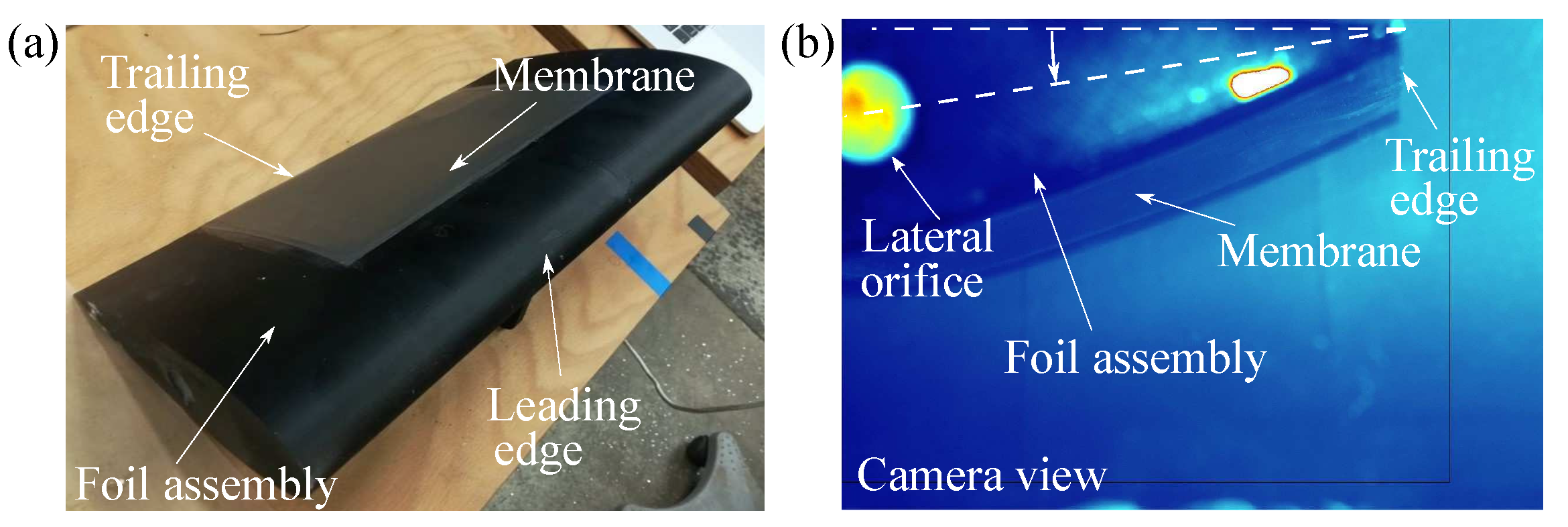
2.1. The Foil Assembly

We manufactured a rigid foil based on an extruded NACA 0025 profile. The chord and the span of the foil were $c=0.20\mathrm{m}$ and $S=0.40\mathrm{m}$, respectively. The foil was 3D printed in ABS and had a cavity inside of its body to allocate the electromagnets and the optosensor. A side view of a cross section of the foil is shown in Figure 1a. In the figure, the cavity, the electromagnets, the optosensor and the membrane are illustrated. The electromagnets controlled the deformation of the membrane and the optosensor measured the deformation of the membrane. The electromagnets were positioned in close proximity to the membrane to generate magnetic pull and to deform the membrane.

A top view of the physical assembly of the foil (without the membrane) is shown in Figure 1b. The figure shows the electromagnets and the optosensor. The cavity was padded with support foams and wooden spars to support the weight of the membrane. The electronic cables of the assembly exited the foil through a lateral orifice. The position of the orifice prevented the cables to obstruct the flow on the suction and pressure sides of the foil. The orifice was filled with silicon to prevent water flooding of the blade.

2.2. The Membrane

The membrane used to seal the foil assembly was an off the shelf membrane manufactured by KEMET. The membrane is a polymer based magnetoelastic membrane designed originally to reduce electromagnetic interference (EMI). The membrane is composed of magnetic powder suspended in a flexible polymer material. Due to its reduced thickness (0.2 mm) and good stiffness to flexibility ratio, it was ideal for our application.

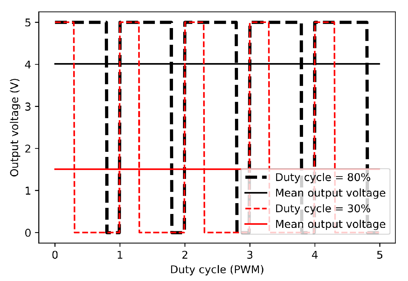
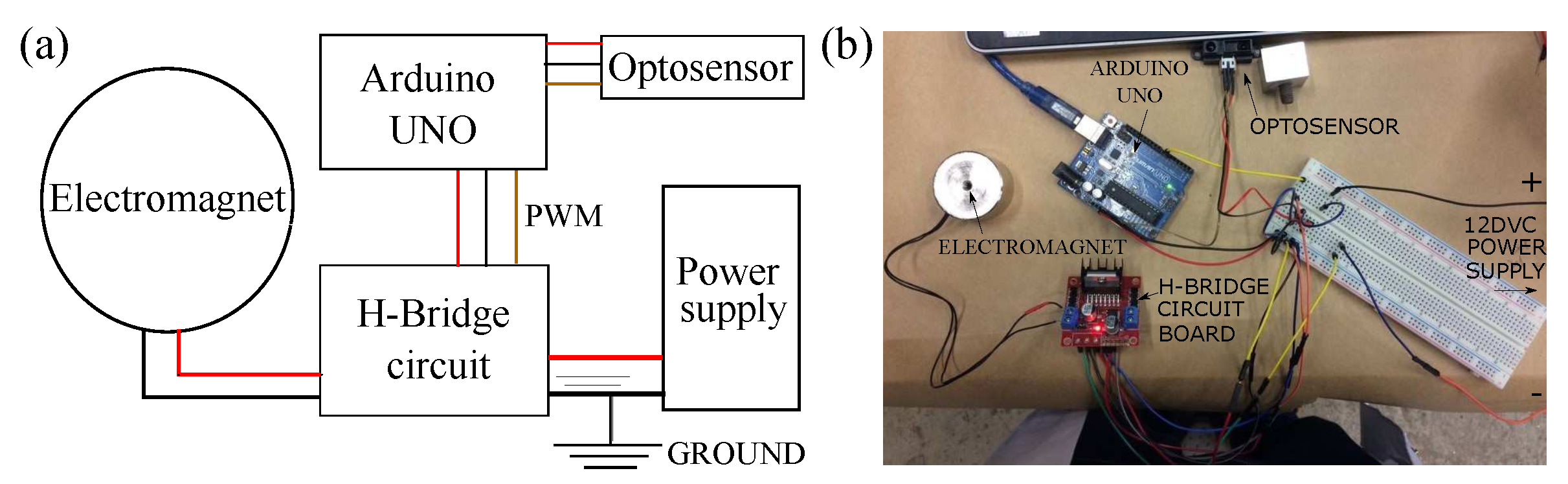
2.3. Membrane Control and Deformation Measurement

The deformation of the membrane was controlled by means of a pulse width modulation (PWM) signal. As shown in Figure 2, different PWM duty cycles are equivalent to different mean output voltage levels. In the figure, for example, two duty cycles of 30% and 80% are shown with dotted red and black lines, and their corresponding mean output voltages (1.5 and 4 VDC) are highlighted in solid red and black lines, respectively. In this example, we note that a 100% duty cycle would be equivalent to 5 VDC.

We note that the 80% and 30% duty cycles shown in Figure 2 are just for illustrative purposes. In our experiment, the duty cycles that were used were 100% and 0%, as indicated in the PWM routine of the Arduino code provided in the supplementary material. In this routine, the PWM value ranges between a byte value of 0 and 255. These two duty cycles were used to alternate the voltage supply of the electromagnets and therefore, the deformation of the membrane. A high voltage (high duty cycle) equated large deformation, whilst a low voltage (low duty cycle) equated reduced deformation.

The PWM signal was generated with an Arduino UNO microcontoller. The PWM signal was connected to an L298N motor driver, which served as the power stepping up unit. The L298N circuit board was powered by an external 12 VDC power supply. We note that the polarity of the wiring for the two electromagnets needed to be the same, since opposite polarity would have cancelled the magnetic field. Hence, the polarity and the pull of the electromagnets was tested before sealing the final assembly.

The Arduino program used to generate the PWM is included as additional material. In the program, the frequency of the actuation is changed by modifying the time delay (DT) between the two duty cycles. Three actuation frequencies were tested: slow, intermediate and fast, with DT = 1000, 500, and 100 ms, respectively. Different DT yields a faster or slower response in the deformation of the membrane, because DT controls the speed at which the output voltage of the electromagnet changes. However, the relationship between DT and the frequency at which the membrane deformation occurs is not known a priori. This is because this relationship is subject to the hardware set up and to the throughput of data in the system. Hence, the relationship between DT and the frequency of the membrane ($f_1$, $f_2$, $f_3$) is quantified experimentally in Section 3.2.

The deformation of the membrane was measured with a 5V DC Sharp reflective sensor. The voltage outputs of the sensor were converted to distances by utilising the voltage distance plot provided in the manual of the sensor. The membrane reflective side was white to maximise reflection.

An schematic and an image of the circuit to control the electromagnet and measure the output signal of the sensor is shown in Figure 3a,b. respectively. In the figures, the main components are: the Arduino UNO, the L298N H-Bridge printed board, the electromagnet and the optosensor. In Figure 3a the red and black wires denote positive and negative polarity, whilst the brown wire denotes a signal. The external power supply depicted in Figure 3a is not visible on Figure 3b. Ground is common to all components of the circuit.

2.4. Water Proofing

Water proofing of the optosensors and electromagnets was performed to protect the electronics in case the cavity was flooded. Hence, the circuitry of the optosensor was coated with varnish. Additionally, silicon was used to cover the exposed wiring connections inside of the cavity of the foil. We note that during the experiments, the operation of the actuation circuit remained in a dry environment. However, water proofing allows for wet operation as well.

2.5. Cost, Safety and Power Requirements

The total cost of the actuation system remained below £100. This contrasts other surface actuation technologies such as piezoelectric actuators and micro fibre composites (MFC), that have higher costs. Besides, these alternative actuation technologies are typically not designed to operate under water. As a reference,

Table 1. Table of costs of actively control membrane circuit.

Component	Cost per Unit	Quantity
Magnetic membrane	£42.90	1
Electromagnet	£8.40	2
Optosensor	£7.83	1
Arduino UNO	£20.40	1
H-bridge motor driver	£6.99	1

shows the detailed costs of the actuation mechanism utilised in this work.

Hence, we consider that the electromagnetic actuator is a good compromise between cost and water operability. Additionally, the range of voltages and required power to operate this system is low compared to other technologies. Piezoelectric bending actuators were found to operate at 60 VDC, whilst MFC required 300 VDC. Since we are operating in water, high voltages could become a safety concern. Therefore, further to water proofing and providing a common ground to all electronics, we consider that the reduced rated power of 3W and low rated voltage of $24\mathrm{VDC}$ of the electromagnets enhance the safety of the experimental tests. At the same time, the system is not energy intensive and could be beneficial for energy harvesting devices, as discussed later in Section 3.4.

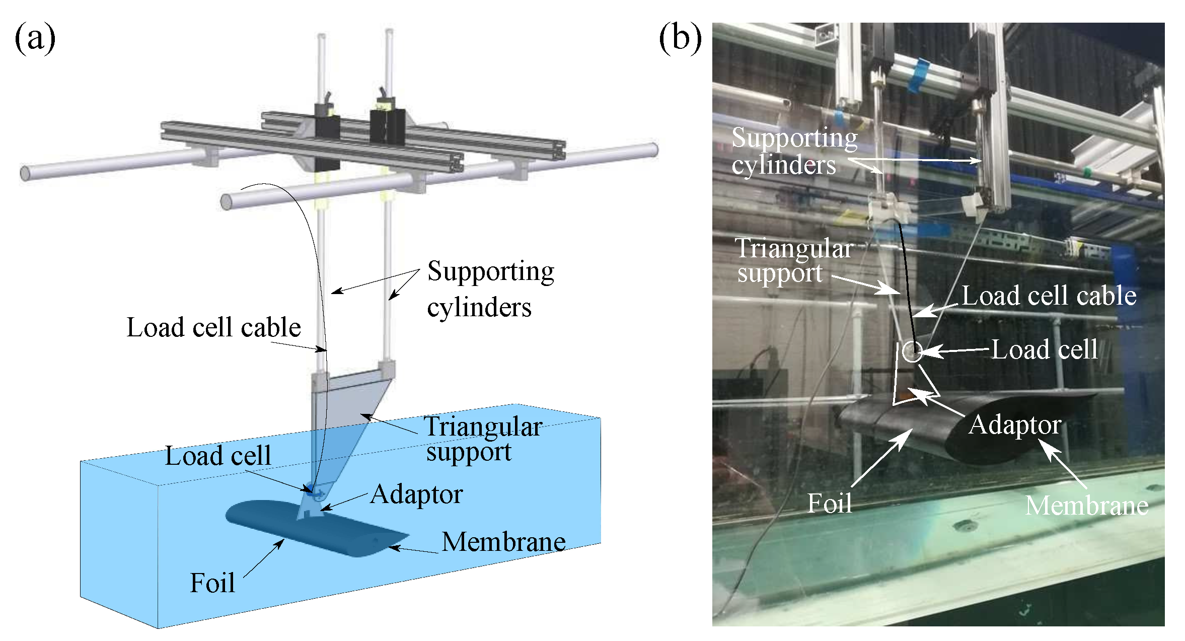
2.6. The Experimental Setup

Figure 4a,b show an schematic and an image of the experimental apparatus, respectively. The rig consisted of a six-mm thick acrylic triangular support, which was connected at its lower end to the cable side of a six-axis load cell. The load cell was connected to an adaptor piece that held the foil in place. The adaptor had two supporting arms that reduced spanwise vibrations of the foil. Load cell measurements were sampled at 1000 Hz and data was acquired for 1 min at low, intermediate and fast actuation frequencies. The rig was held in place with two supporting cylinders, whose vertical position could be modified to set the submergence depth of the foil.

The rig and foil were mounted in a free surface water tunnel at the School of Engineering Sanderson Laboratory, at the University of Edinburgh. The water tunnel is $9\mathrm{m}$ long, $0.4\mathrm{m}$ wide and $0.9\mathrm{m}$ high with a flat, horizontal bed. The mean water depth was set to $0.5\mathrm{m}$ and the blade was placed horizontally $0.25\mathrm{m}$ below the water surface. The span of the foil was sized to fit the width of the flume to promote two-dimensional flow.

The final foil assembly with the membrane is shown in Figure 5a. The foil was surface finished with a coating of matt black paint. The membrane was attached to the foil with silicon rubber around its edges and the actuation operation was tested in air prior to immersion in water. A side view of the foil assembly in the water tunnel is shown in Figure 5b. The lateral orifice, from which the cables exiting the foil, is visible in Figure 5b. Membrane displacements and forces were measured at low, intermediate, and fast actuation frequencies.

The normal ($F_y$) and chordwise ($F_x$) forces were measured and post-processed with a Chebyshev type II low pass filter. The lift (L) and drag (D) forces were computed with

$$L=F_{y}cos\alpha -F_{x}sin\alpha$$

(1)

and

$$D=F_{y}sin\alpha +F_{x}cos\alpha ,$$

(2)

where $F_y$ and $F_x$ are the normal and the chordwise force components of the foil, and $\alpha$ is the angle of attack depicted in Figure 5b. In this Figure, $\alpha$ is defined positive in the counter clockwise direction. The lift and drag coefficients ($C_L,C_D$) were computed by nondimensionalising the force components by $0.5\rho U^{2}A$, where $\rho$ is the water density, U is the freestream velocity, and A is the product of the span and the chord of the foil.

2.7. Testing Conditions

Although the purpose of this manuscript is to develop a low cost system for an oscillating membrane, it is important to contextualise the testing conditions chosen to verify the functionality of the system. The foil was tested at $\alpha ={10}^{\circ }$. The chord based Reynolds number was Re = 100,000. Assuming low turbulence intensity, at these $Re$ and $\alpha$, the separation point of a NACA 0025 is at $x/c\approx 0.20$ [44]. Since the location of the electromagnets is at $x/c=0.60$, the testing condition ensured that the localised actuation of the membrane occurs within the separated boundary layer, similarly to the set-up of Jones et al. [40]. The tested frequencies were $f_1=0.10$ Hz, $f_2=0.30$ Hz and $f_3=0.73$ Hz. The amplitude displacement of the membrane was 1.5 mm and measured with the optosensor. This displacement was obtained by converting the voltage output of the optosensor and by using the voltage distance conversion table of the manufacturer. Frequencies around $f_3$ and amplitudes above 1 mm are enough to notice differences in the aerodynamic or hydrodynamic performance of foils [40]. As such the testing conditions ensures that the mixing in the boundary layer is enhanced and a change in foil performance occurs.

2.8. Error Quantification

The susceptibility of $C_L$ to changes in $\rho$, U and A can be expressed as

$$\delta C_L=\sqrt{{\left[\frac{\partial C_L}{\partial A}\delta A\right]}^2+{\left[\frac{\partial C_L}{\partial L}\delta L\right]}^2+{\left[\frac{\partial C_L}{\partial \rho }\delta \rho \right]}^2+{\left[\frac{\partial C_L}{\partial U}\delta U\right]}^2},$$

(3)

where $\delta A$, $\delta L$, $\delta \rho$ and $\delta U$ are changes in A, L, $\rho$ and U, respectively.

In our experiments, $\delta A=0{\mathrm{m}}^2$, since the span and the chord of the foil remain constant. Previous work by Arredondo-Galeana and Viola [6,45] have shown that changes in the fluid temperature remain below 0.5 ${}^{\circ }$C in this water flume during winter, particularly during the morning hours. As such, we consider $\delta \rho \le 0.001\mathrm{kg}/{\mathrm{m}}^3$. We note that previous tests in the flume have shown that the steady state U is reached after approximately 1 min [31] with the flow running. Hence, the flume was run for 10 min prior to the force measurements. Subsequently, U was measured with laser Doppler velocimetry (LDV). The measurement was taken 1 m upstream of the model at the beginning and at the end of the force measurements. This yielded $\delta U\le 0.001\mathrm{m}/\mathrm{s}$. Additionally, the flume was not shut down until the end of the measurements, to promote a low $\delta U$. Furthermore, once the foil was set at fixed $\alpha$ the only variable that was modified was DT in the Arduino software. Therefore, we consider $\delta L<0.001$ N and $\delta D<0.001\mathrm{N}$, as provided by the load cell manufacturer data sheet. With the above mentioned considerations, we obtain $\delta C_L=0.003$ and $\delta C_D=0.0002$. In order to compute $\delta C_D$, $C_D$ and D replace $C_L$ and L, respectively, in Equation (3).

Lastly, the systematic error in $\alpha$ is approximately ±1${}^{\circ }$. However, this error is constant in all of the force measurements, since the foil position did not change while the membrane was actuated. Therefore this error does not affect the susceptibility analysis.

3. Results

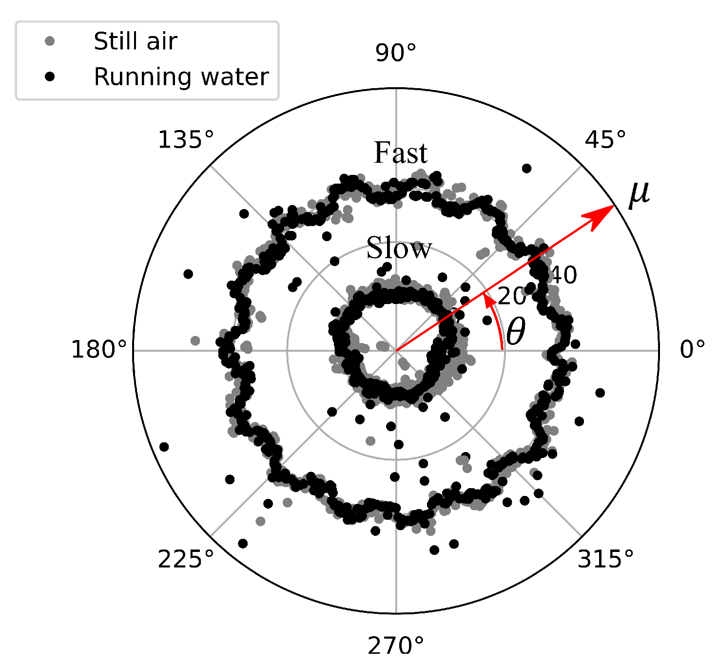
3.1. Membrane Displacement Characterisation

The membrane deformation was measured both in still air and in running water in the water tunnel. Results are presented in Figure 6a,b, respectively. The aim of the test in air was to check the operation of the assembly, whilst the test in water was performed to check that the membrane would deform under hydrodynamic loads. In the figures, the output of the optosensor is plotted for the slow, intermediate, and fast actuation frequencies with black, blue, and red markers, respectively. Figure 6a shows the test in still air, whilst Figure 6b shows the test in running water. In both figures, the intermediate and fast actuation measurements are plotted with a vertical offset of 20 and 40 mm, respectively, whilst the slow actuation measurement does not have an offset.

The membrane deformation ($\mu$) was computed as follows. First, the distance to the membrane was computed from the voltage, which is a function of the distance to the reflective wall that is provided by the manufacturer. Since the optosensor is in near proximity to the membrane, the behaviour is linear and a first order equation was derived to convert voltages to distance in millimetres. Then, the mean distance to reflective wall (without noise) was subtracted from the signals to obtain $\mu$. In this work, $\mu$ is estimated in running water at the slow actuation signal case. The two red horizontal dotted lines in Figure 6b show that the amplitude of $\mu$ is approximately 1.5 mm. The amplitude is assumed to be the same for the intermediate and fast actuation cases, since the two PWM duty cycles are the same for the three deformation cases.

Since the electromagnets were subject to two voltage levels only (see Figure 2), the measured deformation at slow actuation resembles a square wave. Interested readers can find in the supplementary material of the manuscript a video of the membrane deformation in still air. As the actuation frequency increases, the shape of the signal resembles more the shape of a sinusoidal wave. The shape of the deformation could be adjusted if more voltage levels are included in the control algorithm. For the purpose of this study, we expect the fast actuation frequency to show a difference in hydrodynamic performance compared to the slow and intermediate actuation frequencies.

The mean values of the membrane deformation decreased by about 2% when tested in running water, as opposed to the deformation measured in still air. This shows that the effectiveness of the control system is not significantly affected when tested under running water. The spread or width of the optosensor signal also decreased in water, as observed particularly in the slow actuation signals (black markers) of Figure 6a,b. This could be due to additional damping provided by the water to the membrane.

The noise of the membrane deformation measurements in still air and running water are compared in the polar plot of Figure 7. The figure shows a polar plot where the radial coordinate is $\mu$ (membrane deformation in mm) for the slow and fast actuation cases, as shown in Figure 6. The polar coordinate $\theta$ is the phase of one cycle of the slowest actuation case over a range of $0^{\circ }<\theta \le {360}^{\circ }$, where $\theta =0^{\circ }$ is defined as the rising edge of the signal. For the fast actuation case, 7.3 cycles are plotted and the rising edge of the first cycle is plotted at $\theta =0^{\circ }$. For clarity we show the slow and the fast actuation frequencies only. The outer rings correspond to the membrane deformation at fast actuation, whilst the inner rings corresponds to the membrane deformation at slow actuation. Light gray markers denote the tests in still air, while the dark markers denote the tests in running water. In the plot, the phase difference between the air and water signals is removed.

The polar plot confirms that the mean values of the membrane deformation in still air and in running water are similar. It is noted that the noise of the signal increases in water with the flume on, i.e., more outliers are identified in the running water measurements. The outliers, however, are not detrimental to detect the trend in deformation of the membrane. This is visible in the inner circle of the polar plot, where the trend of the deformation is not lost in the running water test. Hence, the results presented here show that submergence an operation in water is not detrimental to the actuation mechanism, despite of the slight increase of noise in the signal.

3.2. Frequency Analysis

Lift and drag forces were recorded for a duration of $60\mathrm{s}$ at the three actuation frequencies. The power spectral density (PSD) of the L and D force measurements, and of the membrane deformation measurement ($\mu$) are plotted versus the Strouhal number ($S_t$) in Figure 8. Fast and intermediate actuation are plotted. Fast actuation is shown in black, whilst intermediate actuation is shown in red. Slow actuation is not plotted since no discernible peaks were detected in the signals. In the figure, the dotted lines correspond to L, the solid lines to D, and the dashed dotted lines to $\mu$. For clarity, the PSD of $\mu$ and L are displaced by a negative and a positive offset, respectively. We recall that $S_t=fc/U$, where f is the frequency, c is the chord of the foil, and U is the free stream velocity.

It can be seen that at fast actuation (black lines) a peak in $\mu$ is detected at around $S_t=0.29$, whilst at intermediate actuation (red lines) the peak is broader and detected around $S_t=0.12$. The peaks are confirmed in the PSD signals of L and D at both fast (black) and intermediate (red) actuation. $S_t=0.29$ and 0.12 correspond to frequencies of $0.73\mathrm{Hz}$ and $0.30$ Hz, respectively. Both $S_t$ are highlighted to the left of the figure with black vertical dotted lines.

We note that considering low Reynolds numbers, the fast actuation $S_t$ is within the range of numbers that have been identified in the literature to increase lift and decrease drag [40]. Hence the most significant changes in lift and drag are expected at $S_t=0.29$. Furthermore, the ratio between the high and intermediate frequency peaks is approximately 2.5 and it corresponds to the inverse ratio of the time delays (DT) utilised in the control algorithm for fast and intermediate actuation. The time delays are DT = 100 ms for fast and DT = 250 ms for intermediate actuation. At slow actuation (DT = 1000 ms), and as mentioned previously, no discernible peak is identified and therefore the signals are not included in the figure. The time delays were specified in the PWM routine of the Arduino UNO code, and the code is available as supplementary material.

According to Yarusevitch et al. [46], the Strouhal number due to vortex shedding of a NACA 0025 at $\alpha ={10}^{\circ }$ is $S_t*=2.5$, where the characteristic length is the projected area of the foil over a plane normal to inflow and given by $c\sin \alpha$. Here, we note that the PSD of the force signals show a peak at $St=14.4$, which is highlighted with a red vertical dotted line to the right of Figure 8. Considering that in this work $\alpha ={10}^{\circ }$, this is equivalent to a $St*=2.5$. Although PIV and wake measurements were not carried out for this work, this comparison shows that vortex shedding could also occur in this modified NACA 0025 foil. The additional peaks, to the left of the vortex shedding $S_t$ could be related to mechanical vibrations in the rig, since these peaks have been detected in the same rig with different geometries by the first author [31], and also possibly due to membrane-fluid interactions.

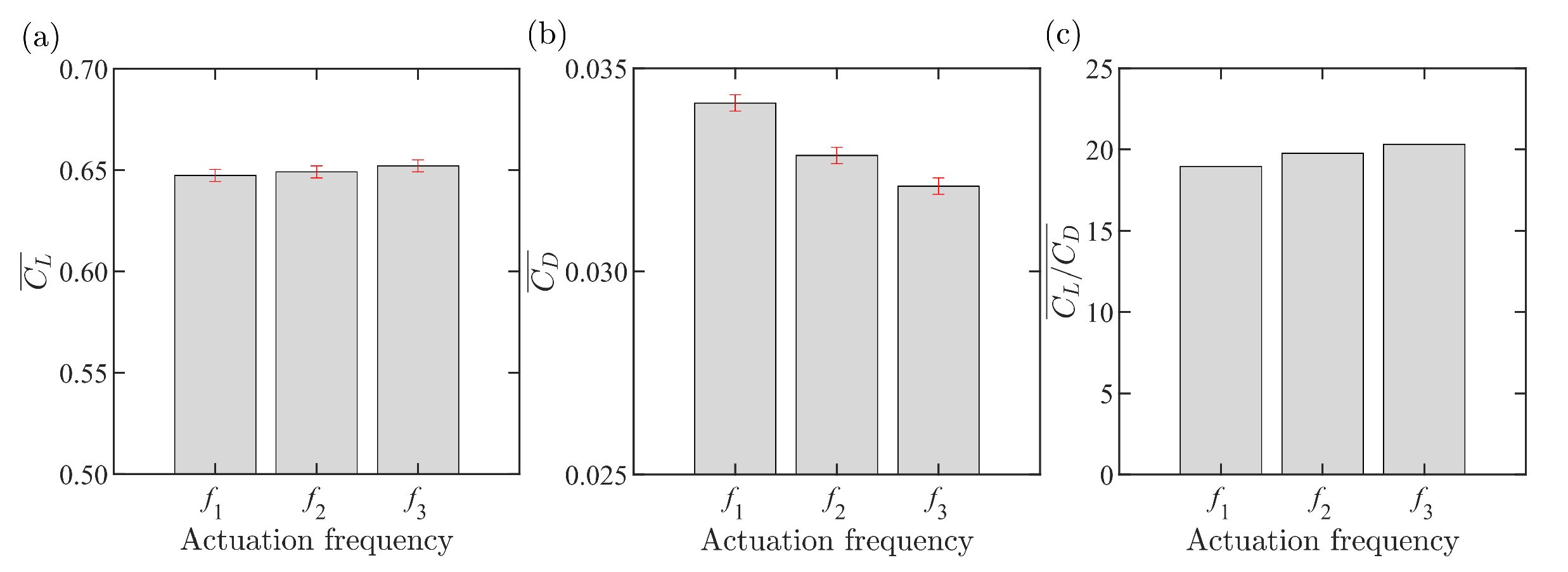
3.3. Time Averaged Lift Coefficient, Drag Coefficient and Lift to Drag Ratio

The measured time averaged $C_L$, $C_D$ and $C_L/C_D$ at $\alpha ={10}^{\circ }$ are shown in Figure 9a–c, respectively. In each subfigure, the three membrane actuation frequencies ($f_1$—slow, $f_2$—intermediate, $f_3$—fast) are shown from left to right. Results in Figure 9a,b show a 1% increase in the mean $C_L$ and a 6% drop in the mean $C_D$, as the membrane actuation changes from $f_1$ to $f_3$. The gain in lift and drop in drag coefficients translate into a $7\%$ gain in the mean $C_L$/$C_D$ ratio. This is shown in Figure 9c, as the actuation frequency changes from $f_1$ to $f_3$. Error bars are included in Figure 9a,b, to highlight $\pm \delta C_L$ and $\pm \delta C_D$, as computed in Section 2.8. It is noted that although the differences in $C_L$ are small, the differences in $C_D$ are significant and surpass the computed error bars.

Results of Figure 9 show that the oscillating membrane has a higher impact in $C_D$ than in $C_L$. Hence oscillating membranes could be complementary to load alleviation technology that modifies $C_L$, for example, passive trailing edge flaps that mitigate peak loading in fluctuating flows [31,47].

It is worth noting that the trend in results presented here are in line with the trends found by Jones et al. [40] at low Reynolds with periodic surface morphing in wind tunnel experiments. We recall however that although the trends are consistent, the actuation mechanism between this study and that from Jones et al. [40] is different and more economical. Here we have used an off the shelf low voltage approach to actuate an electromagnetic membrane under water, as opposed to the use of high voltage macro fibre composites in a wind tunnel.

3.4. Potential Applications of Technology

This section highlights potential applications for actively controlled membranes, such as the one presented in this paper. As such, we identify underwater applications where a reduction of $C_D$ and an increase in the $C_L/C_D$ ratio would be beneficial. We note that although the membrane utilised in this study is not originally designed for underwater applications, it serves as a proof of concept. Hence, this work can help towards the design of a tailored magnetoelastic membrane for underwater applications, in which the actuation principle could be electromagnetic. With this in mind, we now present some examples, where such system could be employed.

3.4.1. Marine Renewable Energy Harvesters

Marine renewables is a growing field, where reduction of the Levelised Cost of Energy (LCoE) and improved reliability are primary goals. Both tidal and wave energy devices aim to harness the energy from the ocean with a diversity of technologies. A few of these technologies utilise blades to generate lift and mechanical power, which is transformed to electric power by a generator. We analyse two examples, in which oscillating membranes could be incorporated to the blades of these devices. First, tidal turbines and secondly, wave cycloidal rotors.

According to Scarlett et al. [13,48], flow separation in a tidal turbine blade can occur throughout the whole span of the blade when the turbine is operated at a suboptimal tip speed ratio ($\lambda$). Due to the unsteady marine environment, optimal operation is not always possible, therefore flow separation through the span of blade is likely to occur. This can result in load oscillations that decrease the fatigue life of the turbine, and in power peaks that require an over-designed power rated generator. Localised oscillating membranes along the span of the blade could help in mitigating these peaks. The membranes could be small inserts on the suction side of the blade and be hydrostatically balanced.

For a 1-MW turbine in large wave conditions, flow separation accounts for about 6% reduction in the power coefficient of a horizontal tidal turbine [13]. For a 1 MW tidal turbine, this translates into 60 kW of loss power. Considering that the type of electromagnet required for the blade would be smaller than a scrap magnet, then the required power for an electromagnetic membrane would be below 60 kW.

Active oscillating membranes could also be beneficial to wave energy harvesters, such as wave cycloidal rotors. These rotors are a technology under recent research and development, due to their power capture potential [15,49,50]. A typical wave cycloidal rotor has its rotor axis aligned parallel to the wave crest and its rotation is driven by a set of blades with uniform cross section. The frequency of rotation is the same as that of the incoming wave, but the phase of rotation is different in order to generate lift on the blades.

Since the blades are of uniform cross section, the full surface of the blade could be made of magnetoelastic material and be hydrostatically balanced. The inclusion of oscillating membranes would prevent losses due to drag, which are estimated to be around 25% of the available energy in a wave [49]. Therefore, for large scale wave cyclorotors (≥0.5 MW), the energy required to actuate the electromagnets would remain below the energy loss due to viscous losses.

3.4.2. Boat Appendages

Boat appendages such as foils and rudders are streamlined and their efficiency (and thus the boat speed) depends on $C_L/C_D$. While rudders are used to manoeuvre the boat, foils are used to lift the hull above water level. Modifications to both rudders and foils have been developed consistently and some examples include flapped rudders, flapped foils, flettner rudders, active rudders, tubercle rudders [51,52].

It is possible to incorporate actively controlled membranes to rudders and foils to improve $C_L/C_D$ and performance. In this case, energy expenditure would be required, however, the actuation system could incorporate systems such as solar panels to make the energy expenditure sustainable.

3.4.3. Autonomous Underwater Vehicles (AUVs)

In autonomous underwater vehicles (AUVs) drag reduction is typically pursued with shape optimisation [53]. Oscillating membranes could help in reducing the drag or resistance generated by the hull of the AUV. Oscillating membranes can also increase the $C_L/C_D$ ratio of the lifting control surfaces. The energy saved in propulsion due to hull drag reduction could be used to balance the energy expenditure in the oscillating membranes. Alternatively, novel energy technologies such as fuel cells could be used to activate the membranes [54].

Hence, the above mentioned applications fall within the solution scope of low cost actively controlled membranes to delay flow separation in an underwater environment and at low Reynolds numbers.

4. Conclusions

It has been shown that actively controlled oscillating membranes can reenergise the boundary layer on the suction side of a foil and delay flow separation. This can increase the lift to drag ratio of foils and blades, by increasing lift and decreasing drag. Most of these studies have been performed for air applications in wind tunnels. Here, we demonstrate for the first time, to the best knowledge of the authors, that such control strategy can also be performed in water at low cost for underwater applications.

To demonstrate the applicability of such control strategy at low cost in water, we covered the suction side of a 3D printed foil with an off the shelf electromagnetic membrane. The membrane was actuated via electromagnets and its deformation measured with an optosensor inside the body of the foil. The performance of the actuation system was tested in still air and in running water. The deformation of the membrane behaved similarly in both of these tests.

The foil was positioned at a fixed angle of attack (${10}^{\circ }$) in the water tunnel to measure the impact of the membrane deformation in the hydrodynamic performance of the foil. Two voltage levels were used to control the electromagnets and the deformation of the membrane, and three actuation frequencies were tested: slow, intermediate, and fast. At fast actuation, when $St=0.29$, the lift increased by $1\%$, whilst the drag and lift to drag ratio dropped by $6\%$ and $7\%$, respectively.

We note that the research data and the proposed technology, describe the processes and measurements of the aerodynamic quality, only within the framework of the placement of the measuring equipment relative to the separation point. In this case the electromagnets were located at $x/c=0.6$. Assuming low turbulence intensity and considering Re = 10,000 and $\alpha ={10}^{\circ }$, the separation point was expected to be around $x/c\approx 0.2$. Therefore, the results presented on this paper do not relate to other chord based Reynolds numbers nor to different positioning of the electromagnets.

The results presented in this work show that oscillating membranes are effective for underwater applications. Importantly, low cost actuation mechanisms such as the one implemented here could be developed for marine applications. Finally, we summarise the realm of possible applications for this type of technology, which include tidal turbines, wave cycloidal rotors, boat appendages, and AUVs, among others.

References

1. Chang, P.K. Separation of Flow; Pergamon Press: London, UK, 1970. [Google Scholar]
2. Carter, J.E.; Vatsa, V.N. Analysis of airfoil leading edge separation bubbles. AIAA J. 1984, 22, 1697–1704. [Google Scholar]
3. O’Meara, M.; Mueller, T.J. Laminar separation bubble characteristics on an airfoil at low Reynolds numbers. AIAA J. 1987, 25, 1033–1041. [Google Scholar] [CrossRef]
4. Stevenson, J.P.J.; Nolan, K.P.; Walsh, E.J. Particle image velocimetry measurements of induced separation at the leading edge of a plate. J. Fluid Mech. 2016, 804, 278–297. [Google Scholar] [CrossRef] [Green Version]
5. Smith, J.; Pisetta, G.; Viola, I.M. The scales of the leading- edge separation bubble. Phys. Fluids 2021, 33, 045101. [Google Scholar] [CrossRef]
6. Arredondo-Galeana, A.; Viola, I.M. The leading-edge vortex of yacht sails. Ocean. Eng. 2018, 159, 552–562. [Google Scholar] [CrossRef] [Green Version]
7. Arredondo-Galeana, A.; Viola, I.M. Force generation mechanisms of downwind sails. In Proceedings of the 7th High Performance Yacht Design Conference, Auckland, New Zealand, 11–12 March 2021. [Google Scholar]
8. Sørensen, J.N. Aerodynamic Aspects of Wind Energy Conversion. Annu. Rev. Fluid Mech. 2011, 43, 427–448. [Google Scholar] [CrossRef] [Green Version]
9. Rezaeiha, A.; Montazeri, H.; Blocken, B. Characterization of aerodynamic performance of vertical axis wind turbines: Impact of operational parameters. Energy Convers. Manag. 2018, 169, 45–77. [Google Scholar] [CrossRef]
10. Abbot, I.H.; Doenhoff, A.E. Theory of Wing Sections: Including a Summary of Airfoil Data; Dover Publications, Inc.: New York, NY, USA, 1959. [Google Scholar]
11. Mueller, T.J.; DeLaurier, J.D. Aerodynamics of small vehicles. Annu. Rev. Fluid Mech. 2003, 35, 89–111. [Google Scholar] [CrossRef]
12. Bahaj, A.; Molland, A.; Chaplin, J.; Batten, W. Power and thrust measurements of marine current turbines under various hydrodynamic flow conditions in a cavitation tunnel and a towing tank. Renew. Energy 2007, 32, 407–426. [Google Scholar] [CrossRef]
13. Scarlett, G.T.; Sellar, B.; van den Bremer, T.; Viola, I.M. Unsteady hydrodynamics of a full-scale tidal turbine operating in large wave conditions. Renew. Energy 2019, 143, 199–213. [Google Scholar] [CrossRef]
14. Smyth, A.; Young, A. Three-Dimensional Unsteady Hydrodynamic Modelling of Tidal Turbines. In Proceedings of the 13th European Wave and Tidal Energy Conference (EWTEC), Napoli, Italy, 1–6 September 2019. [Google Scholar] [CrossRef]
15. Arredondo-Galeana, A.; Shi, W.; Olbert, G.; Scharf, M.; Ermakov, A.; Ringwood, J.; Brennan, F. A methodology for the structural design of LiftWEC: A wave-bladed cyclorotor. In Proceedings of the 14th European Wave and Tidal Energy Conference, Plymouth, UK, 5–9 September 2021. [Google Scholar]
16. Lamont-Kane, P.; Folley, M.; Frost, C.; Whittaker, T. Preliminary Investigations into the Hydrodynamic Performance of Lift-Based Wave Energy Converters. In Proceedings of the 14th European Wave and Tidal Energy Conference, Plymouth, UK, 5–9 September 2021. [Google Scholar]
17. Ermakov, A.; Ringwood, J.V. A control-orientated analytical model for a cyclorotor wave energy device with N hydrofoils. J. Ocean. Eng. Mar. Energy 2021, 7, 201–210. [Google Scholar] [CrossRef]
18. Xiao, Q.; Zhu, Q. A review on flow energy harvesters based on flapping foils. J. Fluids Struct. 2014, 46, 174–191. [Google Scholar] [CrossRef]
19. Kerwin, J.E. Marine Propellers. Annu. Rev. Fluid Mech. 1986, 18, 367–403. [Google Scholar] [CrossRef]
20. Carlton, J.S. Marine Propellers and Propulsion; Butterworth-Heinemann: Oxford, UK, 2018. [Google Scholar]
21. Stark, C.; Shi, W.; Atlar, M. A numerical investigation into the influence of bio-inspired leading-edge tubercles on the hydrodynamic performance of a benchmark ducted propeller. Ocean Eng. 2021, 237, 109593. [Google Scholar] [CrossRef]
22. Jagadeesh, P.; Murali, K.; Idichandy, V.G. Experimental investigation of hydrodynamic force coefficients over AUV hull form. Ocean Eng. 2009, 36, 113–118. [Google Scholar] [CrossRef]
23. Fish, F.E.; Lauder, G.V.; Mittal, R.; Techet, A.H.; Triantafyllou, M.S.; Walker, J.A.; Webb, P.W. Conceptual design for the construction of a biorobotic AUV based on biological hydrodynamics. In Proceedings of the 13th International Symposium on Unmanned Untethered Submersible Technology, Durham, NH, USA, 25 August 2003. [Google Scholar]
24. Gad-el Hak, M. Flow Control: Passive, Active, and Reactive Flow Management; Cambridge University Press: Cambridge, UK, 2000. [Google Scholar]
25. Hansen, K.L.; Kelso, R.M.; Dally, B.B. Performance Variations of Leading-Edge Tubercles for Distinct Airfoil Profiles. AIAA J. 2011, 49, 185–194. [Google Scholar] [CrossRef]
26. Lin, J.C. Review of research on low-profile vortex generators to control boundary-layer separation. Prog. Aerosp. Sci. 2002, 38, 389–420. [Google Scholar] [CrossRef]
27. Young, A.; Farman, J.; Miller, R. Load alleviation technology for extending life in tidal turbines. In Progress in Renewable Energies Offshore—Proceedings of 2nd International Conference on Renewable Energies Offshore, RENEW 2016, 1st ed.; Guedes Soares, C., Ed.; CRC Press: Lisbon, Portugal, 24–26 October 2016; pp. 521–530. [Google Scholar]
28. Józsa, T.I.; Balaras, E.; Kashtalyan, M.; Borthwick, A.G.L.; Viola, I.M. Active and passive in-plane wall fluctuations in turbulent channel flows. J. Fluid Mech. 2019, 866, 689–720. [Google Scholar] [CrossRef] [Green Version]
29. Józsa, T.I.; Balaras, E.; Kashtalyan, M.; Borthwick, A.G.L.; Maria Viola, I. On the friction drag reduction mechanism of streamwise wall fluctuations. Int. J. Heat Fluid Flow 2020, 86, 108686. [Google Scholar] [CrossRef]
30. Tully, S.; Viola, I.M. Reducing the wave induced loading of tidal turbine blades through the use of a flexible blade. In Proceedings of the 16th International Symposium on Transport Phenomena and Dynamics of Rotating Machinery (ISROMAC 2016), Honolulu, Hawaii, USA, 10–15 April 2016. [Google Scholar]
31. Arredondo-Galeana, A.; Young, A.M.; Smyth, A.S.; Viola, I.M. Unsteady load mitigation through a passive trailing-edge flap. J. Fluids Struct. 2021, 106, 103352. [Google Scholar] [CrossRef]
32. Cattafesta, L.N.; Sheplak, M. Actuators for Active Flow Control. Annu. Rev. Fluid Mech. 2011, 43, 247–272. [Google Scholar] [CrossRef] [Green Version]
33. Tuck, A.; Soria, J. Separation control on a NACA 0015 airfoil using a 2D micro ZNMF jet. Aircr. Eng. Aerosp. Technol. 2008, 80, 175–180. [Google Scholar] [CrossRef]
34. Esmaeili Monir, H.; Tadjfar, M.; Bakhtian, A. Tangential synthetic jets for separation control. J. Fluids Struct. 2014, 45, 50–65. [Google Scholar] [CrossRef]
35. Li, Y.; Qin, N. Airfoil gust load alleviation by circulation control. Aerosp. Sci. Technol. 2020, 98, 105622. [Google Scholar] [CrossRef]
36. Li, Y.; Qin, N. Gust load alleviation on an aircraft wing by trailing edge Circulation Control. J. Fluids Struct. 2021, 107, 103407. [Google Scholar] [CrossRef]
37. Corke, T.C.; Bowles, P.O.; He, C.; Matlis, E.H. Sensing and control of flow separation using plasma actuators. Philos. Trans. R. Soc. A Math. Phys. Eng. Sci. 2011, 369, 1459–1475. [Google Scholar] [CrossRef] [PubMed]
38. Greenblatt, D.; Wygnanski, I.J. The control of flow separation by periodic excitation. Prog. Aerosp. Sci. 2000, 36, 487–545. [Google Scholar] [CrossRef]
39. Munday, D.; Jacob, J. Active Control of Separation on a Wing with Oscillating Camber. J. Aircr. 2002, 39, 187–189. [Google Scholar] [CrossRef] [Green Version]
40. Jones, G.; Santer, M.; Debiasi, M.; Papadakis, G. Control of flow separation around an airfoil at low Reynolds numbers using periodic surface morphing. J. Fluids Struct. 2018, 76, 536–557. [Google Scholar] [CrossRef] [Green Version]
41. Olivett, A.; Corrao, P.; Karami, M.A. Flow control and separation delay in morphing wing aircraft using traveling wave actuation. Smart Mater. Struct. 2021, 30, 025028. [Google Scholar] [CrossRef]
42. Li, T.; Li, G.; Liang, Y.; Cheng, T.; Dai, J.; Yang, X.; Liu, B.; Zeng, Z.; Huang, Z.; Luo, Y.; et al. Fast-moving soft electronic fish. Sci. Adv. 2017, 3, e1602045. [Google Scholar] [CrossRef] [Green Version]
43. Shintake, J.; Cacucciolo, V.; Shea, H.; Floreano, D. Soft Biomimetic Fish Robot Made of Dielectric Elastomer Actuators. Soft Robot. 2018, 5, 466–474. [Google Scholar] [CrossRef] [Green Version]
44. Feero, M.A.; Goodfellow, S.D.; Lavoie, P.; Sullivan, P.E. Flow Reattachment Using Synthetic Jet Actuation on a Low-Reynolds-Number Airfoil. AIAA J. 2015, 53, 2005–2014. [Google Scholar] [CrossRef]
45. Arredondo-Galeana, A. A Study of the Vortex Flows of Downwind Sails. Ph.D. Thesis, University of Edinburgh, Edinburgh, UK, 2019. [Google Scholar]
46. Yarusevych, S.; Sullivan, P.E.; Kawall, J.G. On vortex shedding from an airfoil in low-Reynolds-number flows. J. Fluid Mech. 2009, 632, 245–271. [Google Scholar] [CrossRef]
47. Hoerner, S.; Abbaszadeh, S.; Cleynen, O.; Bonamy, C.; Maître, T.; Thévenin, D. Passive flow control mechanisms with bioinspired flexible blades in cross-flow tidal turbines. Exp. Fluids 2021, 62, 104. [Google Scholar] [CrossRef]
48. Scarlett, G.T.; Viola, I.M. Unsteady hydrodynamics of tidal turbine blades. Renew. Energy 2020, 146, 843–855. [Google Scholar] [CrossRef]
49. Siegel, S.; Jeans, T.; McLaughlin, T. Deep ocean wave energy conversion using a cycloidal turbine. Appl. Ocean Res. 2011, 33, 110–119. [Google Scholar] [CrossRef] [Green Version]
50. Cao, Y.; Liu, A.; Yu, X.; Liu, Z.; Tang, X.; Wang, S. Experimental tests and CFD simulations of a horizontal wave flow turbine under the joint waves and currents. Ocean Eng. 2021, 237, 109480. [Google Scholar] [CrossRef]
51. Tupper, E.C. Introduction to Naval Architecture, 5th ed.; Butterworth-Heinemann: Oxford, UK, 2013. [Google Scholar]
52. Troll, M.M.F.; Shi, W.; Stark, C. The influence of leading-edge tubercles on wake flow dynamics of a marine rudder. In Proceedings of the 9th International Conference on Computational Methods in Marine Engineering, Edinburgh, UK (Virtual Conference), 2–4 June 2021. [Google Scholar]
53. Stevenson, P.; Furlong, M.; Dormer, D. AUV shapes—Combining the Practical and Hydrodynamic Considerations. In Proceedings of the OCEANS 2007—Europe, Aberdeen, UK, 18–21 June 2007; pp. 1–6. [Google Scholar] [CrossRef]
54. Weydahl, H.; Gilljam, M.; Lian, T.; Johannessen, T.C.; Holm, S.I.; Øistein Hasvold, J. Fuel cell systems for long-endurance autonomous underwater vehicles—challenges and benefits. Int. J. Hydrog. Energy 2020, 45, 5543–5553. [Google Scholar] [CrossRef]
Figure 1. (a) Side view of blade cross section, with cavity covered by the membrane, (b) Top view of final assembly with cavity, electromagnets, optosensor, supporting foams and wooden spars.
Jmse 10 00077 g001
Figure 2. PWM signal with two different duty cycles, 80% and 30% in black and red dotted lines, respectively. In this example, the maximum output voltage is 5 VDC, hence an 80% duty cycle provides a mean output value of 4 VDC (solid black line), whilst a 30% duty cycle provides a mean output value of 1.5 VDC (red solid line. The frequency of actuation of the electromagnet is controlled by changing the time delay (DT) between the two duty cycle signals.
Jmse 10 00077 g002
Figure 3. (a) Circuit wiring schematic where the red and black wires denote positive and negative polarity, respectively, and the brown wires denotes a signal; (b) image of circuit showing electromagnet, h-bridge circuit (L298N), arduino UNO, optosensor, and power supply. The circuit controlled the frequency of actuation of the electromagnet and therefore the membrane frequency.
Jmse 10 00077 g003
Figure 4. (a) Schematic diagram and (b) photograph of experimental rig to hold the blade showing the acrylic triangular support, the load cell, the adaptor piece and the foil.
Jmse 10 00077 g004
Figure 5. (a) Final assembly of blade showing the membrane at the suction side of the blade and (b) side view from the blade with the membrane at an angle of attack of 10 in the water tunnel.
Jmse 10 00077 g005
Figure 6. Membrane displacement measurements in (a) still air and (b) running water at three actuation frequencies: slow, intermediate, and fast. It is noted that the intermediate and fast actuation measurements are plotted with a vertical offset of 20 and 40 mm, respectively. The slow actuation measurement does not have an offset.
Jmse 10 00077 g006
Figure 7. Polar plot showing membrane deformation ( μ ) in still air and in running water for fast actuation (outer rings) and slow actuation (inner rings). The same offset for the fast actuation case is used as in Figure 6.
Jmse 10 00077 g007
Figure 8. Power spectra density of Lift L (dotted), drag D (solid) and membrane deformation ( μ ) curves at two actuation frequencies, fast (black), and intermediate (red). Frequency peaks are identified at S t = 0.3 at fast actuation, whilst S t = 0.12 at intermediate actuation.
Jmse 10 00077 g008
Figure 9. Time averaged (a) C L , (b) C D and (c) C L / C D of at f 1 , f 2 and f 3 , which correspond to low, intermediate, and fast membrane actuation frequencies, respectively. Error bars for C L and C D are included in the figure.
Jmse 10 00077 g009