Article

A Numerical Study on the Impact of Building Dimensions on Airflow Patterns and Bed Morphology around Buildings at the Beach

by
Paran Pourteimouri
*,
Geert H. P. Campmans
,
Kathelijne M. Wijnberg
and
Suzanne J. M. H. Hulscher
Water Engineering and Management Group, Faculty of Engineering Technology, University of Twente, 7500 AE Enschede, The Netherlands
*
Author to whom correspondence should be addressed.
J. Mar. Sci. Eng. 2022, 10(1), 13; https://doi.org/10.3390/jmse10010013
Submission received: 4 November 2021 / Revised: 16 December 2021 / Accepted: 22 December 2021 / Published: 24 December 2021
(This article belongs to the Special Issue Beach-Dune System Morphodynamics)

Abstract

:
The attractiveness of beaches to people has led, in many places, to the construction of buildings at the beach–dune interface. Buildings change the local airflow patterns which, in turn, alter the sediment transport pathways and magnitudes. This induces erosion and deposition patterns around the structures. In this study, a numerical model is developed using the open-source computational fluid dynamics solver OpenFOAM. First, the model is used to predict the airflow patterns around a single rectangular building. The model predictions are validated with wind-tunnel data, which show good agreements. Second, a reference beach building is introduced and then the building dimensions are increased in length, width and height, each up to three times the reference building dimension. The impact of each dimensional extent on the near-surface airflow patterns is investigated. The results show that the near-surface airflow patterns are least dependent on the length of the building in the wind direction and they depend most on the width of the building perpendicular to the wind direction. Third, the convergence of the third-order horizontal near-surface velocity field is calculated to interpret the impact of changes in airflow patterns on potential erosion and deposition patterns around the building. The numerical predictions are compared with the observed erosion and sedimentation patterns around scale models in the field. The comparisons show satisfactory agreements between numerical results and field measurements.

1. Introduction

Coastal zones worldwide have always been attractive to humans, since they provide a wide variety of valuable resources and recreational activities. Population growth near coastlines leads to an increased demand for construction of restaurants, sailing clubs, holiday cottages and pavilions at the beach–dune interface. Figure 1 shows some typical examples of these structures.
A considerable number of studies indicated that the coastlines worldwide have been modified over millennia by human interventions, and this development is continuously growing [1,2,3,4]. There are complex interactions between airflow patterns, sediment transport and bed morphology on the beach. These interactions vary over a wide range of spatial and temporal scales and determine the shape, size, spacing and alignment of beaches and aeolian sand dunes [5]. The impact of buildings at the beach can be schematized by a loop as in Figure 2.
Buildings at the beach affect local airflow patterns and as a result aeolian sediment transport. These airflow patterns depend on building dimension, geometry, orientation, elevation from ground level, surface roughness and the positioning and distance in a row of buildings on the beach [6]. According to Jackson and Nordstrom [4], the dimensions of a building affect the degree to which a structure acts as an obstacle against wind flow and sediment migration. This affects the ability of airflow or sediment particles to move across the top of the structure or around the lateral sides of the structure. Therefore, buildings at the beach–dune interface locally alter wind flow patterns and change the location of erosion and accretion on the beach [7,8]. At longer time scales, the buildings could potentially change the dynamic state of the adjacent dune system, as they may modify the amount and spatial distribution of aeolian sand supply from the beach to the dune. Dunes provide natural flood protections against storm surges. Therefore, the coastal safety might be affected as dunes become more mobile and variability in height increases. Furthermore, a building could locally increase deposition or cause intensive erosion around the structure. These morphological changes affect the buildings at the beach. They might result in the need for sediment removal or even cause the tilting of the structure that affects the building functionality. Therefore, people move their houses elsewhere due to the excessive erosion and deposition, or change the shape of their houses by constructing on poles, for example, to prevent the buildings’ dysfunctions. The impacts of buildings on wind flow and impacts of wind flow on buildings have been well addressed in the literature, focusing on applications such as pedestrian wind comfort, air pollutant dispersion, heat transfer, natural ventilation and wind-driven snow or rain around buildings. However, only a few studies have been conducted on the effects of building characteristics, specifically the impacts of building dimensions, on near-surface wind flow patterns and bed morphology at the beach. Fackrell [9] and Beranek [10] conducted wind-tunnel studies to investigate wind flow around buildings with various dimensions. Fackrell [9] found that the length of the recirculation region behind the building, which was defined as the distance between the leeward face of the structure and the reattachment point of the separated flow, increases with increasing building width normal to the flow direction as well as with decreasing building length parallel to the flow direction. Martinuzzi and Tropea [11] performed experiments to study the impact of width-to-height aspect ratio, W / H , of surface mounted obstacles on the flow patterns and parameters including windward separation and leeward reattachment lengths. They found that the separation length in front of the obstacle increases with increasing width up to about W / H 6 and then decreases slightly for higher ratios. The indications showed that the reattachment length behind the obstacle increases linearly with increasing width up to about W / H 4 and then asymptotically approaches a constant value.
Considering the impact of roughness elements, similar to buildings, on bed topography, Iversen et al. [12,13] conducted wind-tunnel tests on the sand bed to determine the impacts of obstacles with different dimensions on local aeolian erosion and deposition patterns. They found that the flow patterns and therefore the sand transport, depend considerably on the obstacle aspect ratio which was defined as the ratio of obstacle height to lateral width. Their studies showed that the observed erosion on the windward side of the rectangular object was caused by the formation of a horseshoe-type vortex. In a more detailed study performed by Tominaga et al. [14], sand erosion and deposition patterns around a surface-mounted cube was investigated using a wind-tunnel experiment. The results showed a considerable erosion at the upwind edges of the cube extended downwind along the lateral faces, and a small amount of sand accumulation at the leeward face of the cube. They found that the largest amount of erosion in the streamwise direction, x , occurs at x / H = 0.75 in front of the windward face of the cube, while the largest amount of erosion in the spanwise direction, z , occurs at z / H = 0.85 from the lateral sides of the cube, where H was defined as the cube height. Luo et al. [15] performed wind-tunnel tests to improve the understanding of the airflow patterns downwind of cuboid obstacles and to interpret the formation of the sand shadows observed behind obstacles in arid regions. In their studies, they investigated the impact of obstacle shape ratio on both horizontal and vertical airflow patterns around the structures. The shape ratio was defined as the ratio of the top area of the obstacle to its frontal area normal to the wind direction. Considering H as the height of the obstacle, the measurements showed that the flow begins to reattach and move along the bed surface at some distance between 2.5 H to 3 H from the separation point. They concluded that the formation of the low-velocity bubble downwind the obstacle causes sediment deposition behind the leeward face. Sutton and Neuman [16] studied the impact of vortical structures formed in the vicinity and in the wake of the cylindrical objects on the initiation of sediment transport. Their results show that the two counter-rotating vortices in the lee of the cylindrical objects allow the sediment entrainment to occur at lower wind speeds than that of required far away from the objects and in their wakes. The spacing between the cylindrical objects influences the strength of the two counter-rotating vortices, therefore may cause an increase in the sediment activity around cylindrical objects.
Beyers and Waechter [17] developed a CFD model to investigate the development of wind-driven snowdrifts around buildings. As they noted in their study, it is necessary to take the impacts of flow divergence into account in order to predict the development of snowdrifts realistically, while the commonly used models only rely on the threshold wind shear velocities to derive the snow erosion and deposition patterns around buildings.
The aforementioned studies show that the previous research mainly focused on the general airflow patterns around the buildings. However, the detailed quantitative impacts of building dimensions on near-surface airflow patterns have remained poorly understood, despite their important role in near-surface aeolian sediment transport. In addition, first attempts to find a relation between near-surface airflow patterns and near-surface erosion and deposition patterns around the buildings go back to the experimental work by Luo et al. [15]. However, their study was limited to the airflow patterns behind the obstacles that cause the evolution of sand shadows in arid regions over time. Furthermore, Poppema et al. [18] studied the size of deposition patterns around single buildings of different dimensions. However, their study does lack the detailed information on airflow patterns inducing those patterns.
Therefore, in the present study we systematically investigate the impact of building dimensions on the nature and extent of near-surface airflow patterns and the potential morphological changes induced by those flow fields when buildings are placed at a sand surface. We consider a wide area around the buildings to also capture the deposition patterns like those observed by Poppema et al. [18]. The building dimensions considered are length, width and height. The systematic study means that the building dimension is increased in each direction, while the other two dimensions remain unchanged. The two main research questions this study addresses are: (Q1) What are the detailed quantitative impacts of building length, width and height on near-surface airflow patterns which drive wind-driven sediment transport around buildings?; (Q2) What are the qualitative impacts of building length, width and height, on initial morphologic changes driven by wind around buildings at the beach?
In this paper, first a general description of airflow patterns and complex flow structures around an isolated building or a cube are presented in Section 1.1. In Section 2, the numerical modelling approach is explained. The detailed explanation of the numerical model itself and the validation of the model are provided in Appendix A and Appendix B, respectively. Results related to Question 1, on near-surface airflow patterns around buildings with different length, width and height, are presented in Section 3.1. Results related to Question 2, on the impact of building dimensions on wind-driven erosion and deposition patterns, are presented in Section 3.2. The paper ends with the discussion in Section 4, and conclusions that are presented in Section 5.

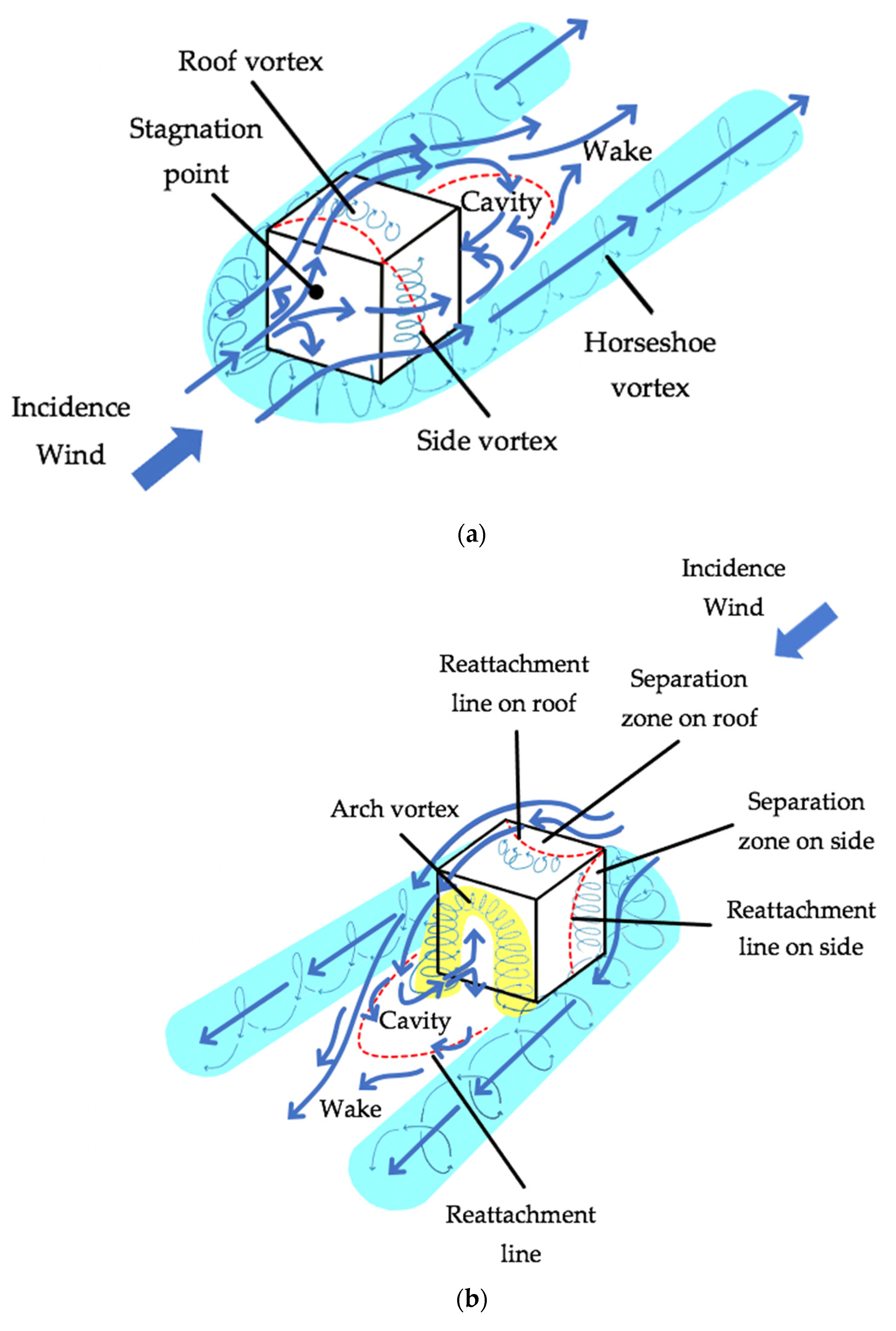
1.1. Wind Flow around an Isolated Building

The wind flow pattern in the vicinity of an isolated building is highly complex. The intrusion of a building, that acts as an impermeable obstacle, into the atmospheric boundary layer causes strong perturbations and complex flow structures in its vicinity. This perturbation is characterized by converting mean kinetic energy to turbulent kinetic energy due to the formation of eddies that are rotating faster or slower than the eddies in the mean flow [19]. Figure 3 shows flow features around an isolated cubical building with an orientation normal to the incident wind flow.
As wind approaches a building, the flow streamlines are deflected over and around the structure which is due to the formation of high-pressure gradients on the windward face. A stagnation point with the highest pressure is formed on the windward face of the building at an elevation approximately two thirds of the building height [20,21]. The location of the stagnation point depends on the building frontal aspect ratio, the height of the building in comparison with the height of the atmospheric boundary layer and the surface roughness upwind of the building [20]. The approaching flow diverges from the stagnation point to the zones with lower pressure including up over the roof, around the lateral sides and down the windward face towards the surface. When the upward and sideward flows encounter the windward edges of the building, they are detached from the surface and flow separation takes place. The separation bubbles on both the roof and the lateral sides of the building are characterized by the reverse flows, low velocity distributions and relatively high turbulence intensities [21]. This happens due to the air suction induced by low-pressure zones on the roof and lateral sides of the building. The detached flow might reattach to the roof or side walls of the building depending on the top and lateral aspect ratios, and upstream surface roughness that determines the turbulence intensity of the incidence flow [20,22]. As mentioned earlier, some of the flow approaching the windward face of the building is deflected downwards to the ground and moves in the reverse direction compared to the incident wind direction. The reversed flow undercuts the incident wind flow and causes it to be detached from the ground level and creates a standing vortex near the bed surface just upstream the windward face of the building [19]. This primary roll-like vortex induces formation of additional vortices that are smaller in size and weaker than the main vortex structure and are eventually connected to the primary vortex around the lateral sides of the building. This vortex is then stretched around the side walls and is extended downwind the building creating a so-called horseshoe-shape vortex, shaded blue in Figure 3 [20].
The flow structures formed behind the building are very complex. The low-pressure zone at the leeward face of the building creates air suction in a so-called cavity region. In this region, the along-wind flow passing over the roof of the building and two horizontally-oriented flows around the lateral sides of the building move in the reverse direction compared to the incidence wind flow, creating a recirculating zone just downstream of the leeward face of the building. The dashed line downstream of the building in Figure 3b shows the end of the cavity region where the streamlines are reattached to the ground surface [19,21]. For a wind incidence angle perpendicular to the upwind face of a cubical building, the height of the cavity region is about 1.5 H , where H is the building height and the length of the cavity region extends to about 2.5 to 3 H , measured from the upstream face of the building. The flow interference increases with increasing building width normal to the wind direction, therefore the cavity region height increases to some extent and its length reaches 12 H for wide buildings with small height-to-width aspect ratios [23]. The horizontal flow patterns behind the rear face of the building show the formation of two counter-rotating vortices that join their extensions at the vertical symmetry plane (yellow shaded vortex in Figure 3b). These spiral vortices entrain some air from the horseshoe-shape vortex, created near the ground level, and whirl it upwards to create a vertically-oriented arch-shape vortex just downstream of the building [11,20,24]. Beyond the cavity region, the reattached flow moving in the direction of approaching flow requires some distance to recover the features of incidence wind flow and release all perturbations, separation impacts and secondary flow structures induced by the presence of building. This occurs in the so-called wake region that is characterized by velocity deficits, higher turbulence intensities and smaller scale eddies compared to the eddies in the incidence wind flow [20,23]. The wake region typically persists to about 5 to 30 H downwind of the building and its height reaches to about 3 to 4 H at a distance of 10 H downstream of the building [19,23].

2. Methods

2.1. Computational Fluid Dynamics (CFD)

In the past few decades, the advances in computing power have led to a significant progress in the application of two and three-dimensional computational fluid dynamics models in wind engineering and aeolian geomorphology [21,25,26]. In CFD models, the flow motion is solved numerically using the Navier–Stokes equations that are a set of partial differential equations including the conservation of mass, conservation of momentum in three dimensions and the conservation of energy. Considering the finite volume method, the computational domain is discretized into a finite number of control volumes and using numerical algorithms, the governing Navier–Stokes equations are integrated over all control volumes. This results in the conversion of partial differential equations into a set of algebraic equations before solving them [27].
For a systematic study of the effect of building dimensions on airflow, application of computational fluid dynamics offers considerable advantages over field measurements and wind-tunnel experiments. The main advantage is that the geometrical design and boundary conditions such as wind speed, incidence angle and shear velocity as well as surface roughness can be changed relatively quickly to systematically analyze the influence of an individual parameter on results. Moreover, the flow field can be solved in very small control volumes that enables the observation of detailed flow features. In addition, CFD simulations avoid scaling issues that might happen in wind-tunnel experiments as the geometrical design can be modelled exactly at the dimensions of interest. This facilitates the validation procedure, since the flow features at the same spatial scales can be compared in both numerical model and experimental results. Furthermore, CFD models avoid the impacts of walls in wind-tunnel experiments, using appropriate boundary conditions. This permits wind flow to leave the computational domain from the lateral sides and the outlet of the domain, and avoids the reflective impacts of walls [21,26,27]. A main disadvantage of CFD is that it can be computationally expensive when increasing the resolution of the computational mesh and/or the size of the computational domain. In practice, the required level of detail and the minimum required three-dimensional space to be simulated, put a limit to the number of cases that are feasible to simulate in a given study.
In this study, a numerical model is developed using OpenFOAM, which is an open-source CFD software. The details of the numerical model including governing equations, turbulence modelling, boundary conditions and initial internal fields are presented in Appendix A of this paper. The model validation is presented in Appendix B of this paper, which shows the capability of the numerical model in predicting the airflow patterns around an isolated building.

2.2. Computational Domain

A three-dimensional rectangular computational domain, shown in Figure 4, is considered for modelling airflow patterns around an isolated building. The definition of the geometric parameters shown in Figure 4, are given in Table 1. Essentially, the scale models of buildings in a numerical wind-tunnel without side wall effects are simulated. We study the impact of relative increases in each dimension, using scale model sized buildings. The dimensions of both the computational domain and the building are selected based on the wind-tunnel experiments performed by Leitl and Schatzmann [28], and their measurements are used in Appendix B of this paper for the model validation. It should be noted that using such a small-scale model in comparison with real buildings at the beach shows the capability of CFD in simulating scaled models. The computational domain inlet is located at x = 0 m , and the domain length, width and height are ( L u + L d ) × 2 W × H , respectively. A rectangular surface-mounted building with the length of l , width of w and height of h is specified within the computational domain, where the building center is located at x = 1 m . The computational domain and the building dimensions are symmetric in the spanwise direction, z . The so-called blockMesh and refineMesh utilities in OpenFOAM are used to create structured hexahedral mesh over the computational domain.
In this study, a computational domain with the length of 3 m , width of 2 m and height of 1.5 m is used. The reference building with the length of l 0 , width of w 0 , and height of h 0 , is considered within the domain. The atmospheric boundary layer parameters are chosen based on the wind-tunnel experiments performed by Leitl and Schatzmann [28] that are presented in Appendix A.3. Considering computational grids with a size almost equal to 0.0125   m and a height of the ground adjacent cells of 0.03   m , the total number of cells in the mesh is approximately 4.57 million. In order to systemati-cally study the impacts of building length, width and height, the reference building is increased in each direction up to three times the reference quantity, while the other two dimensions remain constant. This results in thirteen different simulations as specified in Table 2. It should be noted that the building center in all simulations is located at x = 1 m .

2.3. Methodology for Deriving Bed Level Change from Airflow Patterns

In this study, we are interested in predicting the potential impact of airflow patterns around buildings on the bed level changes of the surrounding area when that area consists of moveable substrate. Commonly used sediment transport models show that the sediment transport rate, q , is proportional to the third-order velocity field ( q U 3 ) [29,30,31,32,33,34,35,36,37,38]. In this study, it is assumed that the sediment will transport at the near-bed wind speed, and it will stay close to the bed. Therefore, as a first step, the vertical component of the velocity field can be neglected, and the sediment transport rate can be written in the following form:
q ( | U H | 2 U H )
where the index H denotes the horizontal near-surface velocity field. The Exner equation states that the temporal rate of change in bed elevation is proportional to the convergence of sediment transport rate:
z b t · q
where z b   [ m ] is the bed elevation, t   [ s ] is the time, and q   [ kg / m s ] is the sediment transport rate. Substituting Equation (1) into Equation (2) gives:
z b t · ( | U H | 2 U H )
Considering Equation (3), a positive convergence of the third-order horizontal wind velocity field in a near-surface plane implies a decrease in sand transport rate hence deposition. Similarly, a negative convergence of the third-order horizontal wind velocity field in a near-surface plane implies an increase in sand transport rate hence erosion:
{ · ( | U H | 2 U H ) > 0                                       D e p o s i t i o n · ( | U H | 2 U H ) < 0                                       E r o s i o n              

3. Results

3.1. Near-Surface Airflow Pattern

The impacts of building dimensions on airflow patterns near the beach surface and the potential implications for bed morphology are investigated. We focus on investigating the impacts of building length, width and height on near-surface airflow patterns, as our main motivation for this work is its implication for sediment transport. Therefore, we show the results of wind velocity magnitude at a horizontal plane close to the bed, i.e., y = 0.0125 m , which is located at an elevation equal to ten percent of the reference building height.
The impact of building length parallel to the incidence wind direction on near-surface wind velocity magnitude is presented in Figure 5a–e. The first glance into the results shows that the building length does not have significant impact on the near-surface airflow patterns adjacent to the building. In order to take a deeper look into results, the effect of building length on the length of the downwind recirculation region just behind the building, L d , which is defined as the distance between the reattachment point of the separated flow and the leeward face of the building, is shown in Figure 5f. It should be noted that the reattachment point at a near-surface plane, y = 0.0125 m , is located on the centerline of the computational domain, where the horizontal component of the velocity, u , changes in sign.
As shown in Figure 5f, the length of the recirculation zone just downstream of the building rear face decreases with increasing building length. This happened due to the reattachment of the detached flow on the roof of the longer building. In order to understand to what extent the velocity deficits due to the presence of the buildings with different lengths continue downwind of the reattachment point, Figure 5g shows the changes in wind velocity magnitude along the domain centerline with respect to the distance from the reattachment point. According to Figure 5g, the wind velocity magnitude increases gradually with increasing distance from the reattachment point until it eventually reaches the undisturbed wind velocity magnitude. Furthermore, the results show that it takes a bit longer distance for the wind to reach a certain speed for the longer building.
Figure 5h shows how streamwise and vertical velocity components change along the domain centerline as the wind approaches the windward face of the building. Figure 5h shows that the near-surface streamwise wind velocity generally decreases with decreasing distance from the windward face of the building, where it changes more rapidly when the distance from the building front face is smaller. The vertical wind velocity is approximately zero until the wind is close the building’s windward face, where a local peak occurs due to the small recirculation region that forms in front of the building and close to the surface. This recirculation develops due to downward deflection of the flow along the front face of the building to the ground, where it deflects again leading to near-bed flow in the opposite direction of the incident wind direction. The results further show that building length has no influence on the length of the upstream area with reduced streamwise wind velocities.
The impact of building width on near-surface wind velocity magnitude is presented in Figure 6a–e. The general flow patterns show that the wider building disturbs a longer and wider area both in front of the windward face and behind the leeward face of the building. Furthermore, the wind velocity magnitude of the flow passing around the windward edges and the lateral sides of the building increases with increasing building width. The reason is that the wind flow approaching the front face of the building is separated into two flow branches in the horizontal plane, passing around the sidewalls of the building. The pressure gradient between the point of separation, in the middle of the building width, and the upwind edges of the wider building is greater, causing the higher wind velocity magnitude values around the windward edges and the lateral sides of the building.
Figure 6f shows the effect of building width on the length of the recirculation region just behind the leeward face of the building, L d . The comparisons between the five different building widths show that the wider building causes the formation of a longer recirculation region just downstream of the building. It can be seen that there is a linear relation between the width of the building and the length of the downwind recirculation zone. The steep slope of the trendline shows that the length of the recirculation zone is highly sensitive to the building width. The results of wind velocity magnitude downstream of the flow reattachment point presented in Figure 6g show that behind a wider building the near surface wind velocity magnitude recovers more slowly over distance from the velocity deficit at the flow reattachment point, where near surface wind velocity magnitude is almost zero.
The changes in streamwise and vertical wind velocities upstream of the windward face of the building are presented in Figure 6h. The results show that the wider the building, the further upwind of the building the minimums of the wind velocity components occur, meaning that the size of the near-bed recirculation region in front of the building increases with increasing building width. Furthermore, it can be concluded from the figure that the streamwise wind velocity deficit for the wider building continue for a longer distance upstream of the building. However, the rate of change decreases with increasing building width. The streamwise wind velocity reaches the undisturbed wind field far away from the building. The negative streamwise wind velocity shows the reversed flow, which depends on the size of the recirculation region in front of the building, and the elevation at which the results were plotted ( y   =   0.0125   m in this study).
The impact of building height on near-surface wind velocity magnitude is presented in Figure 7a–e. The overall flow patterns show more substantial disturbance downstream of the building than upstream of the building. Furthermore, the wind velocity magnitude around the upwind edges and the lateral sides of the building increase considerably with increasing building height. It is obvious that the increase in the near-surface wind velocity magnitude is greater when the building is getting higher in comparison to getting wider. This can be explained by both the pressure gradient and the friction effects that dissipate higher amounts of kinetic energy of the wind flow when passing around the wider buildings. For the wider building, the near-surface flow approaching the building and deflecting towards the lateral sides, travels a longer distance towards the flow detachment at the windward corners of the building compared to the higher building. Therefore, frictional effects act over a longer distance and dissipate higher amounts of kinetic energy of the airflow which, in turn, result in lower wind velocity magnitude around the lateral sides of the wider building. Figure 7f shows that the taller building creates two longer counter-rotating vortices, therefore a longer recirculation region downstream of the building, L d .
The comparisons between five buildings with different heights (Figure 7f) show the high sensitivity of the length of the downwind recirculation zone to building height, however the slope of the trendline shows that the impact of building height on the length of the downwind recirculation zone is smaller than that of building width. As shown in Figure 7g, the influence of building height on the extension of the velocity deficits downwind of the flow reattachment point follows the same pattern as the building width, meaning that the velocity deficits continue for a longer distance from the reattachment point for the taller building. However, the rate of wind velocity magnitude increase over distance is smaller than that for buildings with different widths.
An effect of building height on the streamwise and vertical wind velocities upwind of the building is that a taller building creates the local wind velocity magnitude peak at a larger distance from the windward face of the building (Figure 7h). In addition, Figure 7h shows that the wind velocity magnitude at the center of the recirculation region formed in front of the windward face of the taller building is highest. For the taller building, the wind flow can be less easily released over the building. Therefore, a larger portion of the wind flow moves downwards along the windward face of the building and towards the lateral sides of the building. This implies winds at higher elevation, with higher amount of kinetic energy, move downward. The high-speed downward directed airflow causes the formation of the recirculation region with high-speed magnitudes in front of the taller building. It can be understood from the figure that the length of the low-speed region in front of the building increases with increasing building height, however the rate of change decreases when the building height increases. It is also noteworthy that the magnitude of the local minimum in near-surface windspeed increases with building height to such an extent that there is hardly a difference for the tallest building. The reason is that the flow can move over the smaller building, while more flow blockage happens when the building height increases. This might increase the size of the circulation region in front of the building, and the local minimum in near-surface windspeed.

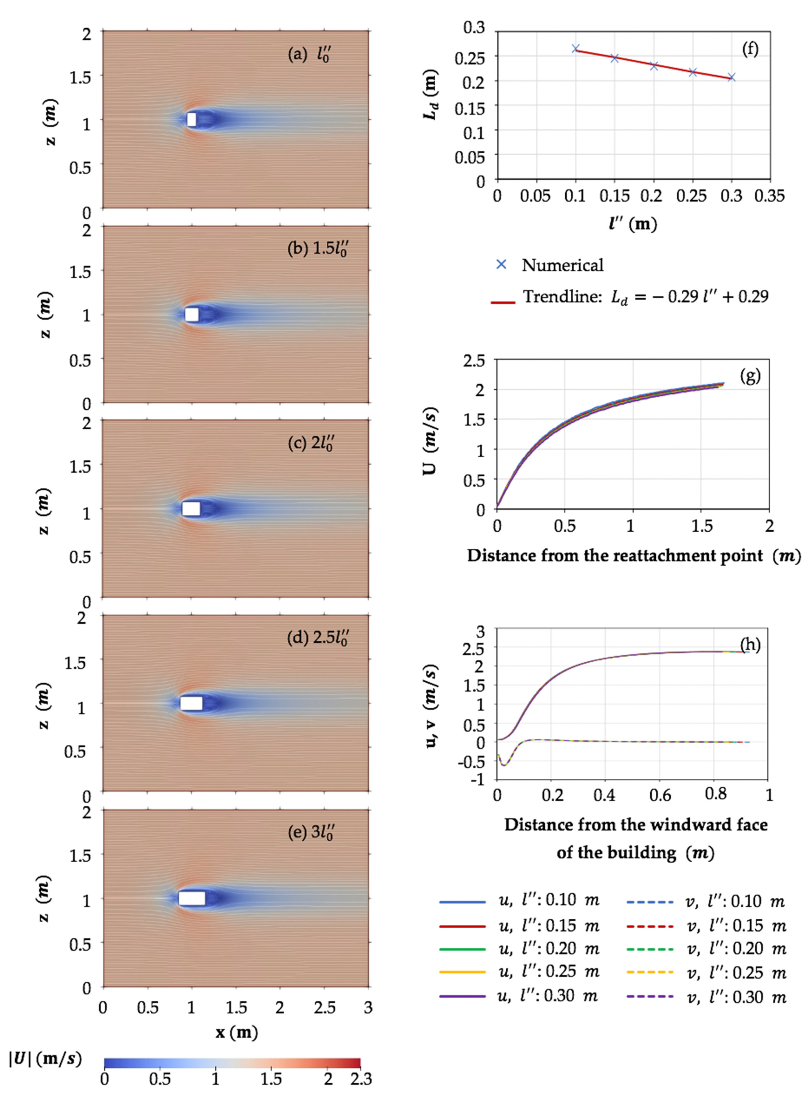
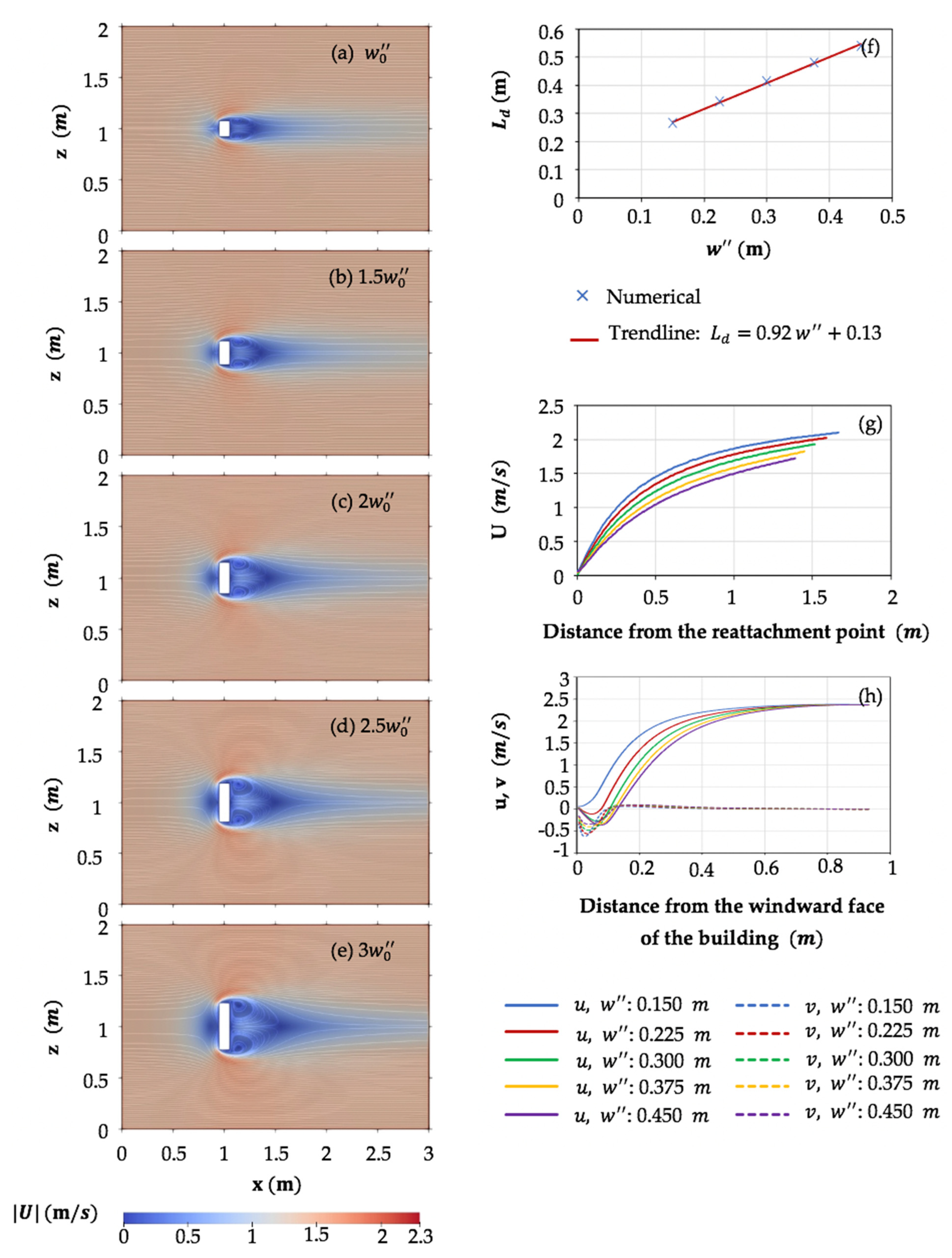
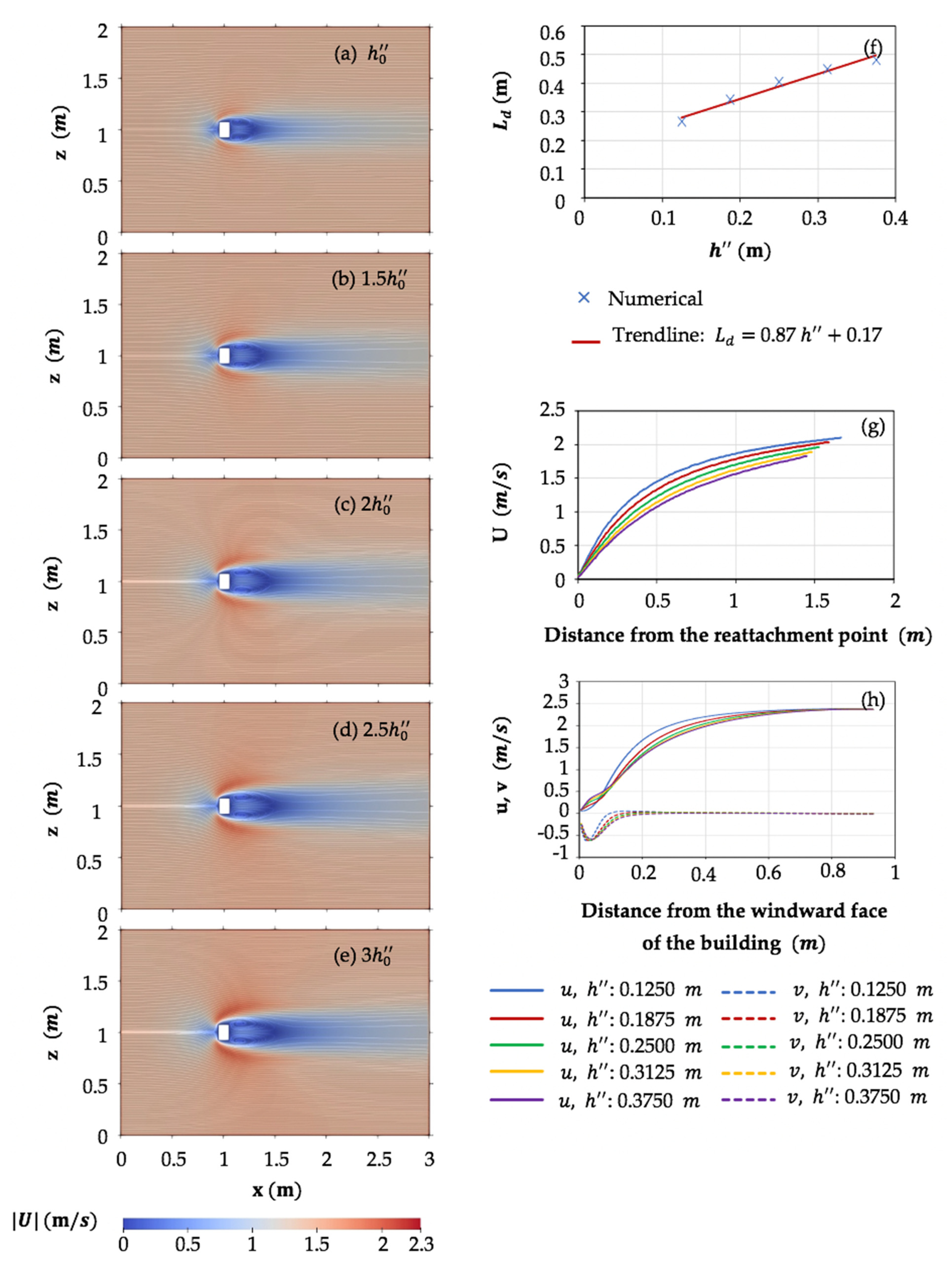
3.2. Impacts of Building Dimensions on Initial Bed Level Change

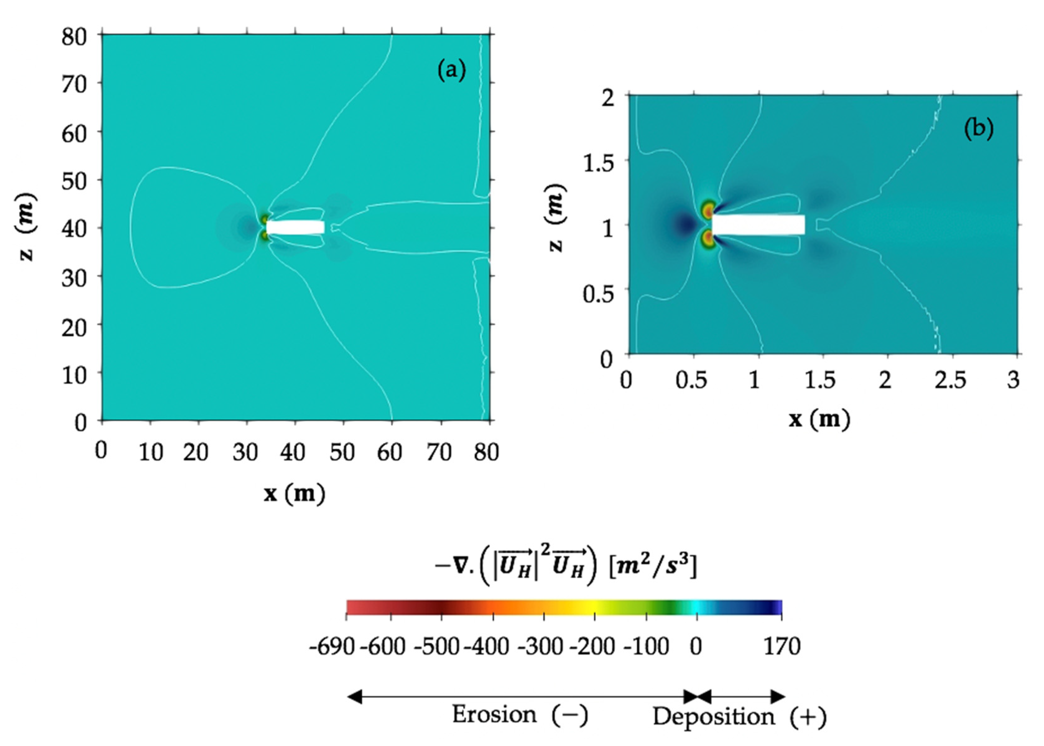
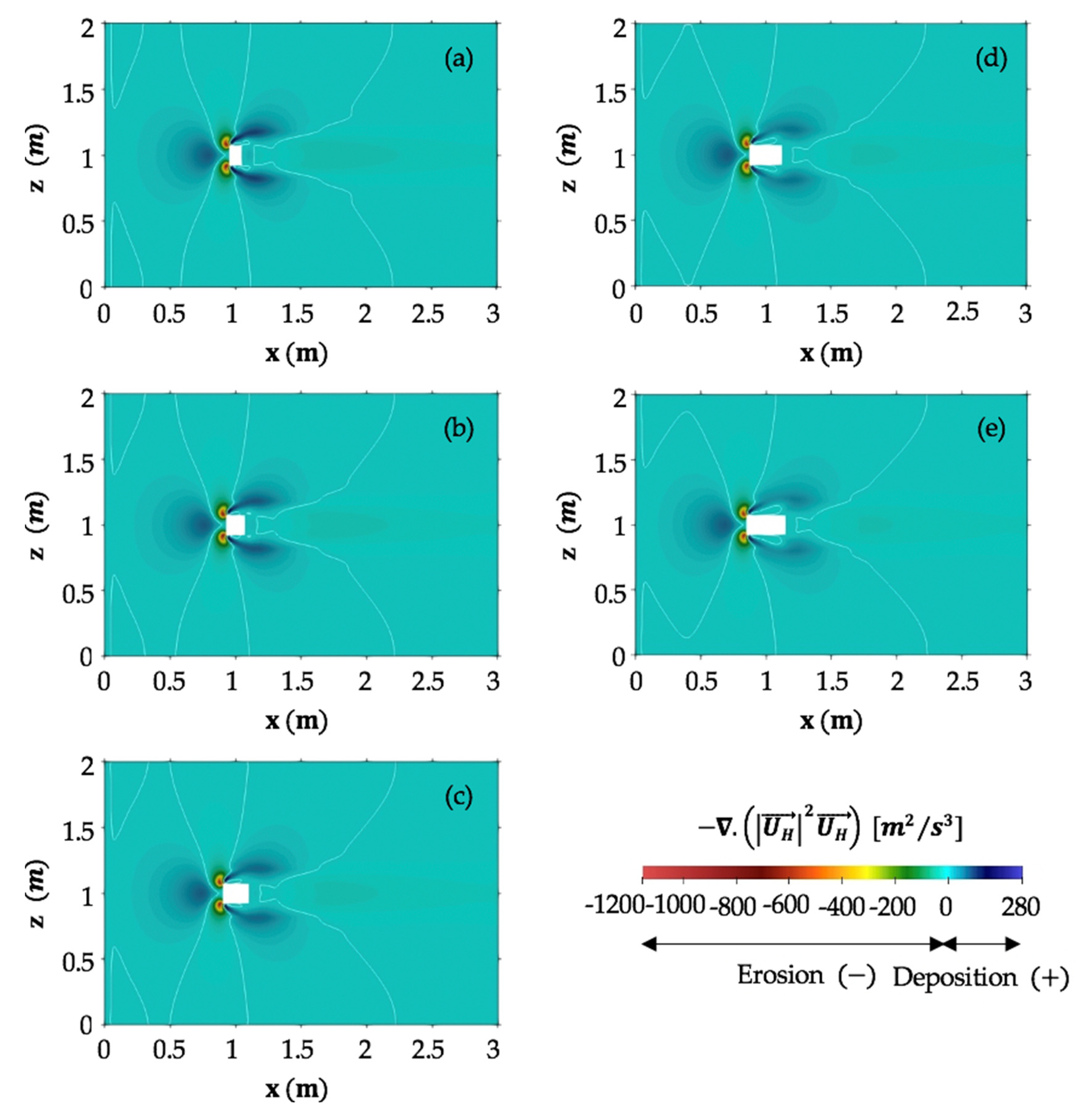
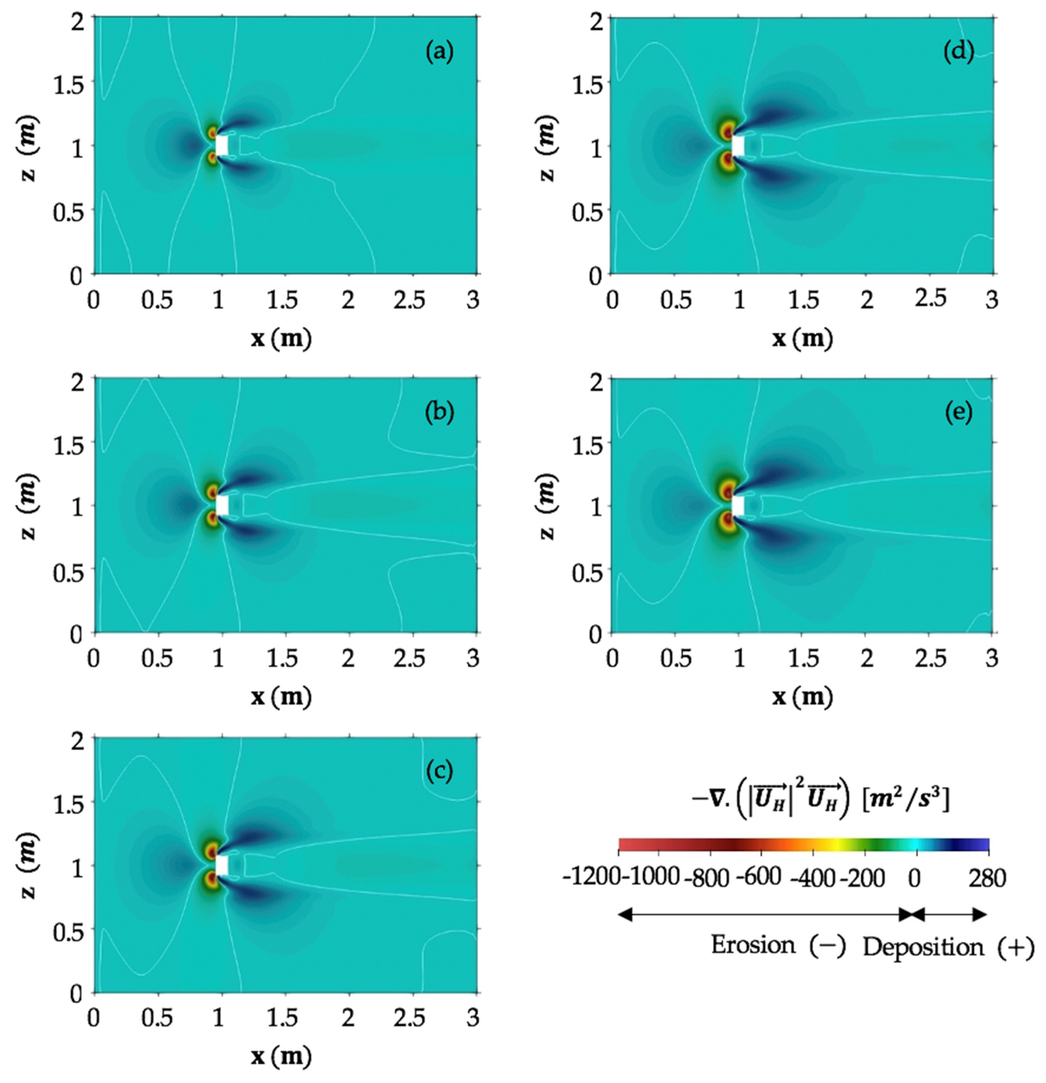
3.2.1. Convergence of the Third-Order Horizontal Near-Surface Flow Field as a Proxy for Initial Bed Level Change

In order to validate the assumption that the convergence of the third-order horizontal near-surface flow field is a good proxy for initial bed level change, and to study the impact of scaling on erosion and deposition patterns around buildings, two new airflow simulations were made. The first simulation is a full-scale building with the length, width and height of 12 m , 2.5 m and 2.5 m , respectively, that is exactly with the same dimension as the full-scale building tested at the Noordwijk beach. It should be noted that he inflow boundary condition for the large-scale simulation are the same as the smaller scale simulations (Appendix A.3). The second simulation is a small-scale building with the length, width and height of 0.72 m , 0.15 m and 0.15 m , respectively. It should be noted that these dimensions were selected in a way to reproduce the same frontal and lateral aspect ratios as the full-scale building tested at the Noordwijk beach. Both full-scale and small-scale numerical model results for the bed level rate of change derived from the convergence of the third-order horizontal wind velocity field at near-surface planes are compared qualitatively to field observations of erosion and deposition patterns around experimental models at the beach (Figure 8 and Figure 9). The full-scale model at the beach near Noordwijk in the Netherlands consists of two shipping containers that were placed besides each other with the total size of 12 m × 2.5 m × 2.5 m in length, width and height, respectively. The containers were placed alongshore and parallel to the dunes with a distance of 20 m from the dune foot. The dominant wind direction was parallel or in a small angle with model’s centerline. A more extensive description of the experimental models at the beach can be found in Poppema et al. [18].
As shown by the yellow to red shaded colors in Figure 8 (both small-scale and full-scale buildings), the highest negative values of the convergence of the third-order horizontal near-surface velocity field occur in a small area around the upwind corners of the building, indicating this location is prone to erosion in case of a moveable bed and the most intensive amount of erosion is expected to happen there. Figure 9a–d show erosion undercutting around the upwind edges of the full-scale container at beach, which is the same pattern as what is predicted based on the numerical model results. Note that the upwind scour zone in front of the building is more strongly developed in the field observations than in the calculated patterns. This might be an effect of topographic feedback, which is absent in the calculations of initial bed level change. The numerical results predict a deposition region upstream of the building (blue shaded colors). Furthermore, two deposition tails starting from some distance away from the lateral sides of the building to downstream of the building form. The field observations given in Figure 9c–f show the same deposition region with lighter colored sand upwind of buildings, which is accompanied with two tails that are formed at some distance from the sidewalls of the building and extended to some extent downstream of the building. It is also seen in both the numerical model results and field observations that erosion happens directly along the lateral sides of the building, bounded on the outside by the inner edges of the deposition tails. The above comparisons show that there is a quite good qualitative agreement between observed and modeled erosion and deposition patterns. This provides support for our assumption that the convergence of the third-order horizontal wind velocity field at a near-surface plane is a suitable proxy for predicting bed level change. Furthermore, the small-scale and large-scale numerical simulations qualitatively show the same patterns of bed morphology, indicating that the overall erosion and deposition patterns are not affected by the scale of the simulation. Therefore, the results of this study are applicable for full-scale buildings at the beach. It is also noteworthy that the erosion and deposition patterns both in the model as well as in the field develop slower for the larger scale buildings. Furthermore, the actual rates of erosion and deposition around buildings depend on the proportionality coefficient in Equation (1). It should be noted that the shape and the dimension of the erosion and deposition patterns around buildings do not depend on the proportionality coefficient.

3.2.2. Relation between Building Dimensions and Patterns of Wind-Driven Bed Level Change

The results of the convergence of the third-order horizontal wind velocity field at a near-surface plane are derived for the previously mentioned simulations specified in Table 2. The impact of building length on bed morphology is investigated using Figure 10. The two deposition tails that form at some distance from the lateral sides of the building to downstream increase in length, while the deposition rate decreases with increasing building length (see the blue-shaded colors with positive convergence). Furthermore, the eroding regions that occur between the lateral sides of the building and the inner boundary of the deposition tails increase in size when the building length increases (see the zero contour lines). The overall results show that the impact of building length on the convergence pattern of the third-order horizontal near-surface velocity field around the building is small. Therefore, it is expected that the magnitude of the building length does not have a large effect on the bed morphology that develops around the building.
Figure 11 shows the impact of building width on bed morphology. The figure shows that for all five tested building widths, the most intensive erosion is expected to happen around the upwind edges of the building. The results show that when the building width increases, the spatial extent of the deposition region in front of the upwind face of the building increases too, and the two deposition tails become slightly longer and wider. The rate of deposition however slightly decreases as the building becomes broader, both in front of the building and in the deposition tails. In addition, the deposition rate just behind the leeward face of the building slightly increases as the building width increases (see the small areas with darker blue-shaded colors just behind the building). It is also noteworthy that initially the erosion is maximum at the centerline behind the building. However, as the building gets wider, the maximum erosion splits and the erosion rate at the centerline reduces in magnitude and regions of deposition start to form.
The impact of building height on bed morphology is investigated using Figure 12. Results show that the areal extent of the upwind erosion around the windward edges of the building increases with increasing building height. Furthermore, it is revealed that an increase in building height leads to a substantial reduction in the deposition rate upwind of the building. However, the area with deposition (darker blue-shaded colors) in front of the building increases in spatial extent with increasing building height. The downstream and lateral extension of the two deposition tails increases when the building becomes taller. These implications can be explained by Figure 7a–e, where the higher wind velocity magnitudes occur around the upwind edges and lateral sides of the taller building. This higher-speed wind flow erodes more sediment particles upwind the building and carries them for a longer distance downstream of the building. Therefore, it is probable that when the building increases in height, a shift occurs from mainly sedimentation in front of the building to mainly sedimentation in the tails. In addition, Figure 12 shows that the rate of sand accumulation in a small area just behind the leeward face of the building slightly increases when the building height increases.

4. Discussion

In the present study, a CFD model using OpenFOAM was developed to investigate the impacts of building dimensions, specifically building length, width and height on near-surface airflow patterns and bed morphology. The numerical results of the flow field around the building were consistent with the observed flow patterns by Martinuzzi and Tropea [11] and Leitl and Schatzmann [28]. Similar to the observations by Martinuzzi and Tropea [11], we found that the size of the near-bed recirculation region in front of the building increases with increasing building width. This can be realized by comparing the length of the local peaks shown in Figure 6h. Furthermore, the results of the present study shown in Figure 6f, indicates that the downstream reattachment length increases linearly with building width, which is consistent with the findings by Fackrell [9] and Martinuzzi and Tropea [11]. It should be noted that these findings are based on tested simulations with certain range of width-to-height aspect ratio up to about four, w / h 4.
For the bed surface of the numerical domain, representing a sandy bed, a uniform aerodynamic roughness length, y 0 , was assumed based on the wind-tunnel experiments performed by Leitl and Schatzmann [28]. This assumption leads to some inconsistencies with the real condition on the beach that can be considered as the model limitations. On dry enough parts of the beach, sand ripples can form over time under windy conditions, changing the bed roughness and therefore the near-surface airflow changes. However, the good agreements between the model predictions of the erosion and deposition patterns with field observations indicate that ripples do not affect the overall patterns, but they might only modify the spatial extents.
The convergence of the third-order horizontal near-surface wind velocity field was used in this study as a proxy for initial bed level change, because in commonly used sediment transport models the sediment transport rate is assumed to be proportional to the third-order velocity field. Strictly speaking, this assumption is only valid for a situation with transport limited conditions; however, on the beach supply limited conditions also occur due to the effects of moisture [39,40,41] which may affect the rate at which bed level changes develop. Moisture may affect the amount of sediment in transport approaching the building. This may specifically affect the rate at which deposition patterns around a building develop. In the extreme condition, if no sediment is in transport at all due to very wet conditions, no deposition patterns can develop because there is no sediment in the airflow. Furthermore, moist beach surface around the building itself may affect the rate at which building induced erosion occurs, hence it takes more time for erosive features to develop. In addition, in this study, the threshold wind speed was not taken into account. It should be noted that if the wind speed becomes less than the threshold wind speed at which the sediment particles start moving, no sediment transport will happen. Figure 13 shows the results of the convergence of the third-order horizontal wind velocity field at a near-surface plane when the wind approaches the building at higher wind velocity magnitude, u r e f = 17   m / s (compared to u r e f = 6   m / s in Figure 8a). The results show that at higher wind speeds where the majority of the domain is well above the threshold wind speed, the similar erosion and deposition patterns develop. It should be noted that the rate of development of patterns increases with increasing the wind velocity magnitude (compared to Figure 8a).
McKenna Neuman and Bédard [42] showed that the fluid perturbation and the system of vortices that develop around buildings depend on the integration between both buildings and the bed surface. In the present study, we used steady airflow patterns around buildings to infer initial effects on bed morphology, hence morphological feedback was not taken into account in this approach. Nevertheless, the erosion and deposition patterns predicted by the numerical model showed good agreement with field observations around the full-scale model and the small-scale model at the beach. The model results showed a considerable erosion around the windward edges of the building, extending less intensively than at the edges along the lateral sides. In addition, the deposition region in front of the upwind face of the building and two deposition tails starting away from the lateral sides of the building and extending downstream of the building occur in all simulations. These findings are similar to the observations by Iversen et al. [12,13], Tominaga et al. [14] and Poppema et al. [18].
To consider the impact of scaling on numerical results shown in this study, the erosion and deposition patterns between a full-scale model and a small-scale model at the beach were compared qualitatively. The comparisons showed that the erosion and deposition patterns that develop around the buildings are not influenced when the scale of the simulation increases. However, the rate of growth of the patterns decreases with increasing the scale of the simulation. This is also valid for small-scale and full-scale experimental models at the beach.
The initial morphological changes predicted by the model show a central downwind deposition just behind the leeward face of the building starts to appear when the building width increases (see Figure 11). The reason is that two horizontal counter-rotating vortices become stronger as the building width increases (see Figure 6a–e). These two vortices push the air towards the centerline behind the building. The air gets pushed upward resulting in an upward component of the wind. On the other hand, the vertical recirculation just behind the building generates a downward motion at the position above the deposition region. For wider buildings, the upward effect of the two horizontal vortices becomes stronger than the downward effect of the vertical vortex which leads to a net upward flow. The net upward flow results in positive convergence of third-order horizontal velocity field at a near-surface plane. Therefore, the erosion and deposition patterns show the formation of a deposition region just behind the leeward face of the wider building.
In this paper we studied buildings on a flat sand surface, whereas on an actual beach buildings are often built in front of a dune. Although dune topography was not included in the simulations, some preliminary implications of building dimensions for sand supply from the beach to the dunes may be formulated from the presented results. The convergence patterns in the near-surface flow field induced by the building demonstrate that ambient sand transport will be captured by the building, both upwind and in two downwind tails. The rate of deposition in the two tails varies with building dimension. If we assume these trends prevail also in the presence of dune topography downwind of the building, such higher rate of deposition would mean an increasingly higher deposition on the dune front at the tail location. From our results of the deposition patterns downstream of the buildings, it can then be derived that the highest building is expected to give the strongest local increase in deposition at the dune front and the longest building the least. Note that this holds for situations with predominantly onshore wind. The ridge-like deposition in front of the wider building increases in size as the building becomes broader. In addition, the eroding region around the windward edges of the building increases substantially with increasing the building height. These might lead to buildings’ mis-functioning and probably tilting that forces the owners of beach buildings to consider measures to smooth the surface or prevent the development of these patterns.

5. Conclusions

In this study, the impacts of building dimensions on near-surface airflow patterns were investigated as well as the implications for bed morphology in the case of a surrounding sandy bed. Specifically, three building characteristics were studied: the building length parallel to the incident wind direction, building width perpendicular to the incidence wind direction and building height. For this purpose, a CFD model using OpenFOAM was developed. The numerical model predictions showed satisfactory agreement with wind-tunnel data of vertical and horizontal wind velocity profiles in the vicinity of the scale model of buildings, providing confidence in the capability of the model to predict the detailed airflow patterns around an isolated building at the beach.
Using this model, a systematic investigation revealed the effects of building length, width and height on airflow patterns at a horizontal plane close to the bed. The results on the relation between building dimensions and near-surface airflow patterns were consistent with those found in Martinuzzi and Tropea [11] as well as Iversen et al. [12,13], where width and height of the building were most influential in the extent and nature of near-surface airflow patterns around the building and downwind length least. Only the length of the recirculation region just behind the leeward face of the building decreases slightly when the building increases in length. This was consistent with findings in Fackrell [9]. By focusing on near-surface flows both in front of the building and downstream of the building, our simulations further revealed that a wider building disturbs a longer and wider region both in front of the building and downstream of the building. The distance at which the upwind deceleration of the airflow starts as it approaches the building increases with building width. The numerical results presented in this study highlighted that with increasing building height, the length of the two counter-rotating vortices just behind the leeward face of the building increases considerably, and with it the length of the recirculation region. Furthermore, with taller buildings it takes a longer distance for the near-surface wind leeward of the building to increase its speed back to the undisturbed wind velocity magnitude.
The convergence of the third-order horizontal near-surface wind velocity field was used as a proxy for sediment transport rate. Although inferred erosion and deposition patterns technically only relate to initial bed level changes, it was found that these compared well to those observed around a full-scale model and a small-scale model at Noordwijk beach and De Zandmotor beach in the Netherlands (Poppema et al. [18]).
As for the near-surface airflow patterns, the initial bed morphology was most dependent on the building width normal to the incidence wind direction as well as the building height, and least on the length of the building parallel to the incidence wind direction. In addition, it was found that for all studied building dimensions, the most intensive erosion is expected to happen around the upwind edges of the building, where the undercutting was observed in the field experiments. The initial bed morphology revealed that the areal extent of these eroding regions directly adjacent to the windward edges of the building increases when the building becomes taller. By focusing on the initial deposition patterns around buildings, the numerical simulations highlighted that the deposition tails downstream of the buildings develop more slowly as the building length increases. Furthermore, sediment deposition that occurs in front of the upwind face of the building becomes larger in spatial extent, and the length of the two deposition tails downstream of the building slightly increases as the building becomes broader. The deposition rate both in the ridge-like deposition in front of the building and in the deposition tails slightly decreases with increasing building width. This implies that the wider the building, the broader and shallower the deposition region in front of the windward face of the building. A small area of sand accumulation appears just behind the leeward face of the building as the building width increases. The numerical results further revealed that with increasing building height the sedimentation rate further upwind of the building decreases, while it increases in the downwind tails.

Author Contributions

Conceptualization, P.P., G.H.P.C. and S.J.M.H.H.; methodology, P.P., G.H.P.C. and S.J.M.H.H.; software, P.P.; validation, P.P.; formal analysis, P.P.; investigation, P.P.; writing—original draft preparation, P.P.; writing—review and editing P.P., G.H.P.C., K.M.W. and S.J.M.H.H.; visualization, P.P.; supervision, G.H.P.C., K.M.W. and S.J.M.H.H.; project administration, K.M.W. and S.J.M.H.H.; funding acquisition, K.M.W. All authors have read and agreed to the published version of the manuscript.

Funding

This research was funded by Netherlands Organisation for Scientific Research (NWO) (contract number ALWTW.2016.036) and co-funded by Rijkswaterstaat (RWS) and Hoogheemraadscap Hollands Noorderkwartier (HHNK).

Institutional Review Board Statement

Not applicable.

Informed Consent Statement

Not applicable.

Data Availability Statement

The study did not report any data.

Acknowledgments

This research is part of the ShoreScape project, which is a joint research project of the University of Twente and Delft University of Technology. ShoreScape focuses on sustainable co-evolution of the natural and built environment along sandy shores. We would like to thank Sander Vos for inviting us in the Noordwijk experiments and Ir. Daan Poppema for discussions and the photo of his scale model experiments at the Zandmotor.

Conflicts of Interest

The authors declare no conflict of interest.

Appendix A. Development of the Numerical Model

Appendix A.1. Governing Equations

In this study, a three-dimensional numerical model is developed using OpenFOAM. The wind flow in this model is considered as incompressible, since for the flow with Mach numbers less than 0.3, the change in flow density is negligible and the divergence of flow velocity can be considered zero [43]. The Mach number is a dimensionless parameter, defined as the ratio of the speed of flow to the speed of sound in the surrounding flow [41]. The Mach number of 0.3 corresponds to the airflow with the speed of about 100 m / s in its normal condition, which is typically greater than the wind speed [44]. In addition, considering the Reynolds number criteria, the wind flow in this study is assumed fully turbulent. Therefore, among all available OpenFOAM solvers for incompressible flows, the so-called simpleFoam solver is selected, which is recommended for steady state simulation of turbulent flows.
The simpleFoam algorithm solves the Reynolds-averaged Navier–Stokes (RANS) equations for turbulent flows using the finite volume method (FVM). The RANS method employs the Reynolds decomposition of flow variables into mean and fluctuating parts, and solves the additional Reynolds stresses that appear in the momentum equations of flow using a turbulence model [27,43,45]. Considering that the conservation of energy is only applied for compressible flows, the governing equations of the three-dimensional flow field can be expressed by continuity and momentum equations that can be written in their steady states as follows:
U = 0
( U U ) = p k + ( υ e f f U )
where U = ( u ,   v ,   w )   [ m / s ] is the three-dimensional flow velocity vector; p k   [ m 2 / s 2 ] is the kinematic pressure, defined as the ratio of the static pressure, p s   [ Pa ] , to the flow density, ρ   [ kg / m 3 ] ; υ e f f   [ m 2 / s ]   is the effective kinematic viscosity, defined as the sum of the kinematic viscosity of the flow, υ   [ m 2 / s ] , and the turbulent (eddy) kinematic viscosity, υ t   [ m 2 / s ] , which is calculated from the turbulence model. In the present study, the kinematic viscosity of the air, υ, is considered as 1.4 × 10 5   m 2 / s .
Although Equations (A1) and (A2) introduce 4 equations and 4 unknowns ( u ,   v ,   w ,   p k ) , they are difficult to be solved numerically. The main reason is that there is an equation for each component of the flow velocity, but there is no equation for the pressure. It should be noted that the continuity equation plays a role of restriction for velocity components, meaning that the computed velocity components from Equation (A2) must satisfy the Equation (A1). In addition, the wind flow in this study is considered as incompressible, therefore the equation of state cannot be used to compute the pressure, as the flow density and temperature are assumed constant. The next reason is that the convective term in the momentum equation, ( U U ) , is non-linear which makes the solution of abovementioned equations more complex. The simpleFoam solver uses the SIMPLE (semi-implicit method for pressure-linked equations) algorithm to solve the continuity and momentum equations.

SIMPLE Algorithm

The SIMPLE algorithm uses an iterative procedure, where the intermediate velocity field is first calculated by solving the momentum equation for an initial guessed pressure field. The intermediate velocity field does not satisfy the continuity restriction. Deriving and solving the pressure equation, the so-called Poisson equation, from the continuity and momentum equations result in a pressure corrector that is used for adjusting the intermediate velocity field and obtaining a new velocity field, that satisfies the continuity restriction after doing several iterations [27,45,46].
The first step to initiate the SIMPLE approach is to express the momentum equation, Equation (A2), in the matrix form as follows:
A U = p k
where A is the known matrix of coefficients that its components are calculated using the discretization of the partial differential terms in the momentum equation. Note that the nonlinearity of the advection terms will involve some kind of linearization method. The above equation includes 3 n equations, where n is the total number of control volumes and each equation is written for the centroid of each control volume. The second step is to decompose the matrix of coefficients, A , into diagonal and non-diagonal components:
A U = B U C
where B and C are the known diagonal and non-diagonal components of matrix A , respectively. Substituting Equation (A4) into Equation (A3) and rearranging the momentum equation in terms of the flow velocity yields the following equation:
U = B 1 C B 1 p k
The third step is to derive the pressure equation, Poisson equation, by substituting the above equation into the continuity equation, Equation (A1), that can be written in the following form:
( B 1 p k ) = ( B 1 C )
In the next step, the iterative procedure starts with an initial guess for the pressure field, p k * . Using the guessed pressure field, the momentum equation is solved to compute the intermediate velocity field, U * = ( u * ,   v * ,   w * ) . This intermediate velocity field does not satisfy the continuity restriction until the solution has been converged. The correct pressure field, p k n , is then obtained by solving the Poisson equation. Subsequently, the pressure corrector, p k , is calculated by subtracting the guessed pressure field from the correct pressure field, p k = p k n p k * . Then, the velocity field is updated, U n = ( u n ,   v n ,   w n ) , using the momentum equation and is checked for the continuity restriction. If the updated velocity field does not satisfy the continuity restriction, a new iteration cycle will start, using p k as the initial guess and U n for the calculation of the matrix of coefficient. The iteration continues until convergence occurs. In this case, the continuity restriction is satisfied in each control volume of the computational domain and the pressure corrector becomes zero [46].

Appendix A.2. Turbulence Modelling

Using the RANS method to solve the Navier–Stokes equations introduces additional unknowns, so-called Reynolds stresses, into the main equations. To close the set of equations, a turbulence closure model must be applied. In this study, the well-known standard k ε model proposed by Launder and Spalding [47] is used. The standard k ε model is a two-equation model based on the Boussinesq approximation. It assumes that the impacts of turbulence on flow can be expressed by an increased kinematic viscosity, and the additional Reynolds stresses can be related to the mean velocity gradients of flow by the turbulent (eddy) kinematic viscosity, υ t [43]. This turbulent kinematic viscosity can be formulated by the turbulence kinetic energy, k   [ m 2 / s 2 ] , and its rate of dissipation, ε   [ m 2 / s 3 ] , as follows [48]:
υ t = C μ k 2 ε
where C μ   [ ] is a dimensionless constant.
In the standard k ε model, the k and ε are computed from their transport equations that can be written in their steady states as follows [27,45]:
( k U ) = ( υ e f f , k k ) + P k ρ ε
( ε U ) = ( υ e f f , ε ε ) + C ε 1 P k ε ρ k C ε 2 ε 2 k
where C ε 1   [ ] and C ε 2   [ ] are dimensionless constants; P k   [ kg / m · s 3 ] is the production of turbulent kinetic energy; and υ e f f , k   [ m 2 / s ] and υ e f f , ε   [ m 2 / s ] are defined as below:
υ e f f , k = υ + υ t σ k
υ e f f , ε = υ + υ t σ ε
where σ k   [ ] and σ ε   [ ] are dimensionless constants. The first and second terms in Equations (A8) and (A9) represent the transport of k or ε by advection and diffusion, respectively; while the last two terms show the rate of production and the destruction of k or ε , respectively. The empirical model coefficients for the standard k ε model are given in Table A1 [47,49]. It should be noted, in the SIMPLE algorithm, the transport equations of k and ε are solved just after computing the updated velocities and the check for the continuity restriction. The turbulent (eddy) kinematic viscosity, υ t , is then updated and be used in the momentum equation for the next iteration cycle.
Table A1. Values of the empirical constants in the standard k ε model [47,49].
ParameterValue
C μ   [ ] 0.09
C ε 1   [ ] 1.44
C ε 2   [ ] 1.92
σ k   [ ] 1.00
σ ε   [ ] 1.30

Appendix A.3. Boundary Conditions and Initial Internal Fields

Considering neutral stratification conditions, fully-developed profiles of mean wind speed, U , and turbulence quantities including turbulence kinetic energy, k , and turbulence dissipation rate, ε , are applied at the inlet of the computational domain shown in Figure A1, using the following equations proposed by Richards and Hoxey [48]:
U ( x = 0 , y , z ) = u * κ ln ( y y g + y 0 y 0 )
k ( x = 0 , y , z ) = u * 2 C μ
ε ( x = 0 , y , z ) = u * 3 κ ( y y g + y 0 )
where u *   [ m / s ] is the friction velocity, κ   [ ] is the von Karman constant defined as 0.41 in OpenFOAM, y   [ m ] is the vertical coordinate, y g   [ m ] is the minimum y-coordinate or the ground level, y 0   [ m ] is the aerodynamic roughness length, and C μ is the dimensionless constant in the standard k ε model defined as 0.09.
The height of the computational domain is significantly smaller than the atmospheric boundary layer (ABL) height, therefore the friction velocity in Equations (A12)–(A14) can be assumed constant with height [50], and is calculated using the following equation proposed by Richards and Hoxey [48]:
u * = κ   u r e f ln ( y r e f + y 0 y 0 )
where u r e f   [ m / s ] is the reference velocity at a reference height, y r e f   [ m ] .
In the present study, the values of the ABL parameters used in inlet profiles are selected based on the wind-tunnel experiments performed by Leitl and Schatzmann [28]. These values are given in Table A2.
Table A2. Values of the atmospheric boundary layer parameters used in inlet profiles [28].
ParameterValue
y g   [ m ] 0.0000
y 0   [ m ] 0.0007
u r e f   [ m / s ] 6.0000
y r e f   [ m ] 0.5000
The analytical inlet profiles of mean wind speed, U , turbulence kinetic energy, k , and turbulence dissipation rate, ε , proposed by Richards and Hoxey [48] are shown in Figure A1.
A zero-gauge pressure boundary condition is applied at the outlet of the computational domain. The no-slip boundary condition for the velocity is used for the bottom of the computational domain and the building walls. It assumes that the speed of the wind flow in direct contact with the bottom of the domain and the walls of the building is identical to the speed of movement of these boundaries, which is equal to zero. Furthermore, the free-slip boundary condition is used for the top and lateral boundary surfaces of the computational domain for all scalar and vector quantities.
The initial internal fields for pressure and velocity are chosen zero, while the initial internal fields for turbulence kinetic energy and turbulence dissipation rate are calculated using the following equations [27,47,48]:
k = 1 2 ( u 2 + v 2 + w 2 )
ε = C μ 0.75   k 1.5 l
where u   [ m / s ] , v   [ m / s ] and w   [ m / s ] are fluctuating components of velocity in the x , y and z directions, respectively; C μ is the dimensionless constant in the standard k ε model defined as 0.09; and l   [ m ] is the turbulence length scale or the characteristic length for the macroscale of turbulence.
Assuming an isotropic inlet turbulence, u = v = w , and estimating the fluctuations to be 5 percent of the reference velocity at the inlet of the computational domain, and selecting l = 0.32   m for the turbulence length scale based on the wind-tunnel experiments performed by Leitl and Schatzmann [28], the initial internal values of the turbulence kinetic energy, k , and the turbulence dissipation rate, ε , are calculated as 0.135 m 2 / s 2 and 0.0255 m 2 / s 3 , respectively.

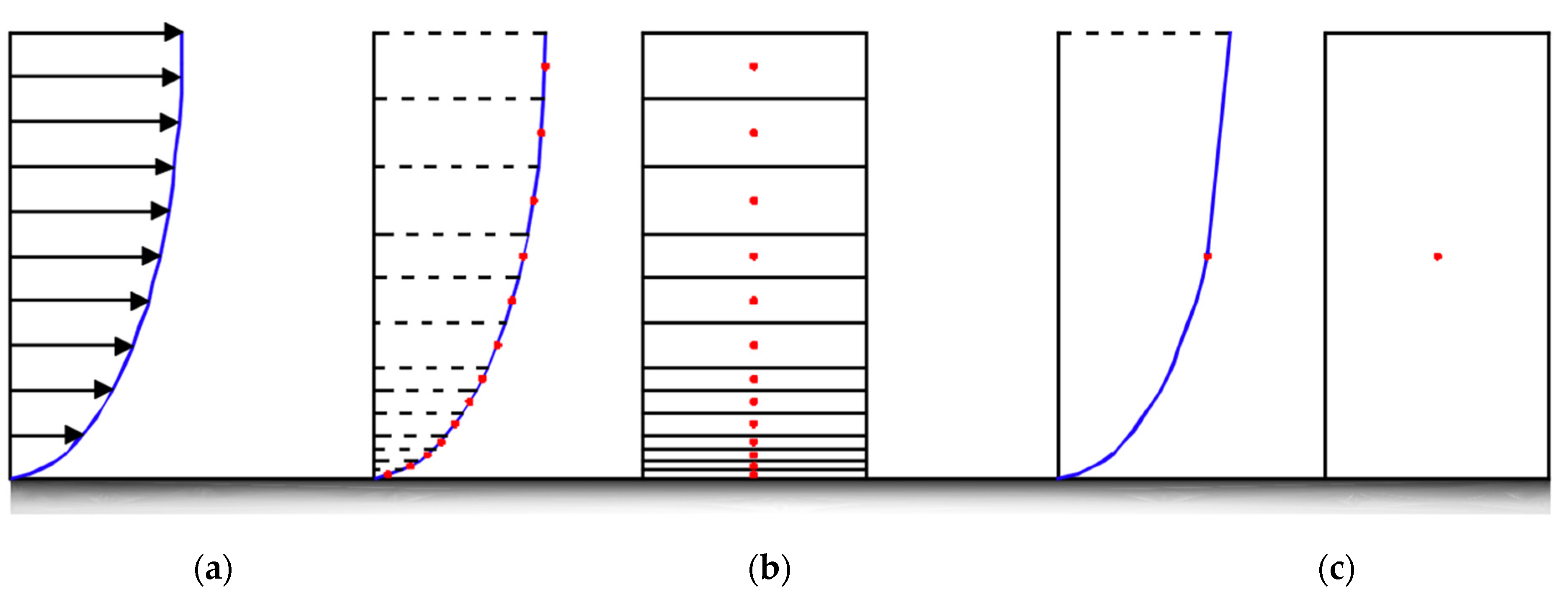
Appendix A.4. Wall Functions

As mentioned in Appendix A.3., the vertical wind velocity profile changes from zero at the bottom of the computational domain, due to the no-slip boundary condition, to its free stream value far away from the wall (see Figure A2a). The largest gradients of the velocity occur in the near-wall region, where the velocity profile becomes quite steep. To accurately simulate the flow behavior close to the wall, it is important to precisely capture the velocity variations in the near-wall region. Using a second-order accurate finite volume discretization method in the OpenFOAM model, the flow features are calculated for the cell centers and the variation of variables is linear between the cell centroids. Therefore, the standard method to accurately simulate the flow in the near-wall region is to gradually decrease the mesh size when approaching the wall boundary [51,52] (see Figure A2b). Applying a very fine mesh close to the wall significantly increases the number of cells, that increases the computational time considerably. Furthermore, increasing the mesh resolution normal to the wall results in the formation of cells with high aspect ratios. The skewness of the cells causes poor cell qualities that increases the instabilities of the CFD solution.
An alternative way to accurately resolve the high velocity gradients close to the wall is to replace a single large cell instead of those thin cells in the near-wall region and introduce a function, so-called wall function, to reproduce the high velocity variations between the cell centroid and the wall boundary [51] (see Figure A2c). Using the wall function approach, the number of cells and therefore the computational time decreases considerably. In addition, the stability of the CFD solution increases significantly.
Considering the universal law of the wall based on the experimental measurements of fully developed turbulent channel flows, the variation of dimensionless tangential velocity close to the wall, U + = U / u τ , with the dimensionless distance normal to the wall, y + = y u τ / υ , is derived. The u τ   [ m / s ] is the wall friction velocity or the characteristic velocity based on the wall shear stress as the velocity at wall is zero. It can be different from u * , and is calculated using the following equation [50,53]:
u τ = τ w ρ
where τ w   [ N / m 2 ] is the wall shear stress; and ρ is the flow density. The near-wall region is then subdivided into three distinct layers as follows [54,55]:
  • Viscous layer for 0 < y + < 5
  • Buffer layer for 5 < y + < 30
  • Inertial layer for 30 < y + < 200
Figure A1. The analytical inflow conditions of (a) mean wind speed, (b) turbulence kinetic energy, k , and (c) turbulence dissipation rate, ε .
Jmse 10 00013 g0a1
Figure A2. Methods of simulating wind flow velocity in the near-wall region (a) The typical vertical wind velocity profile with high velocity gradients close to the wall, (b) Standard linear method, and (c) Wall function approach.
Jmse 10 00013 g0a2
Wall functions are empirical functions that are best fitted to the observed flow behavior close to the wall. The standard wall functions are a linear and a logarithmic function that precisely reproduce the flow behavior in the viscous layer and the inertial layer, respectively. These wall functions can be expressed by the following equations [52,56]:
U + = y +
U + = 1 κ ln ( E y + )
where κ is the von Karman constant defined as 0.41 in OpenFOAM; and E   [ ] is an empirical wall roughness coefficient defined as 9.8 in OpenFOAM. The abovementioned wall functions for viscous and inertial layers intersect in the buffer layer at approximately y + =   11.225 , so-called y l a m + in OpenFOAM. The following conditional statement is then applied in the OpenFOAM model to predict the flow behavior in the near-wall region:
U + = { y +                                                 i f   y + y l a m +   1 κ l n ( E y + )                     i f   y + > y l a m +  
It should be noted, the Equation (A21) cannot precisely predict the flow behavior in the buffer layer, therefore it is not recommended to placing cells in this region.

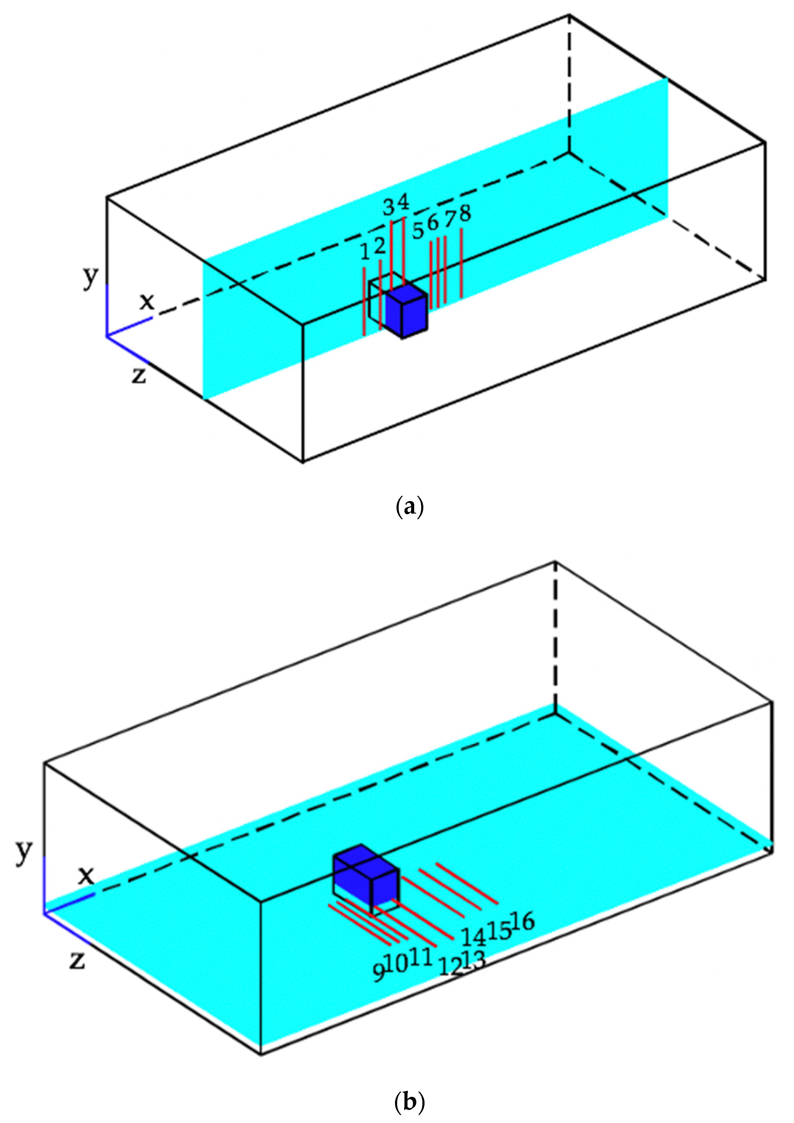
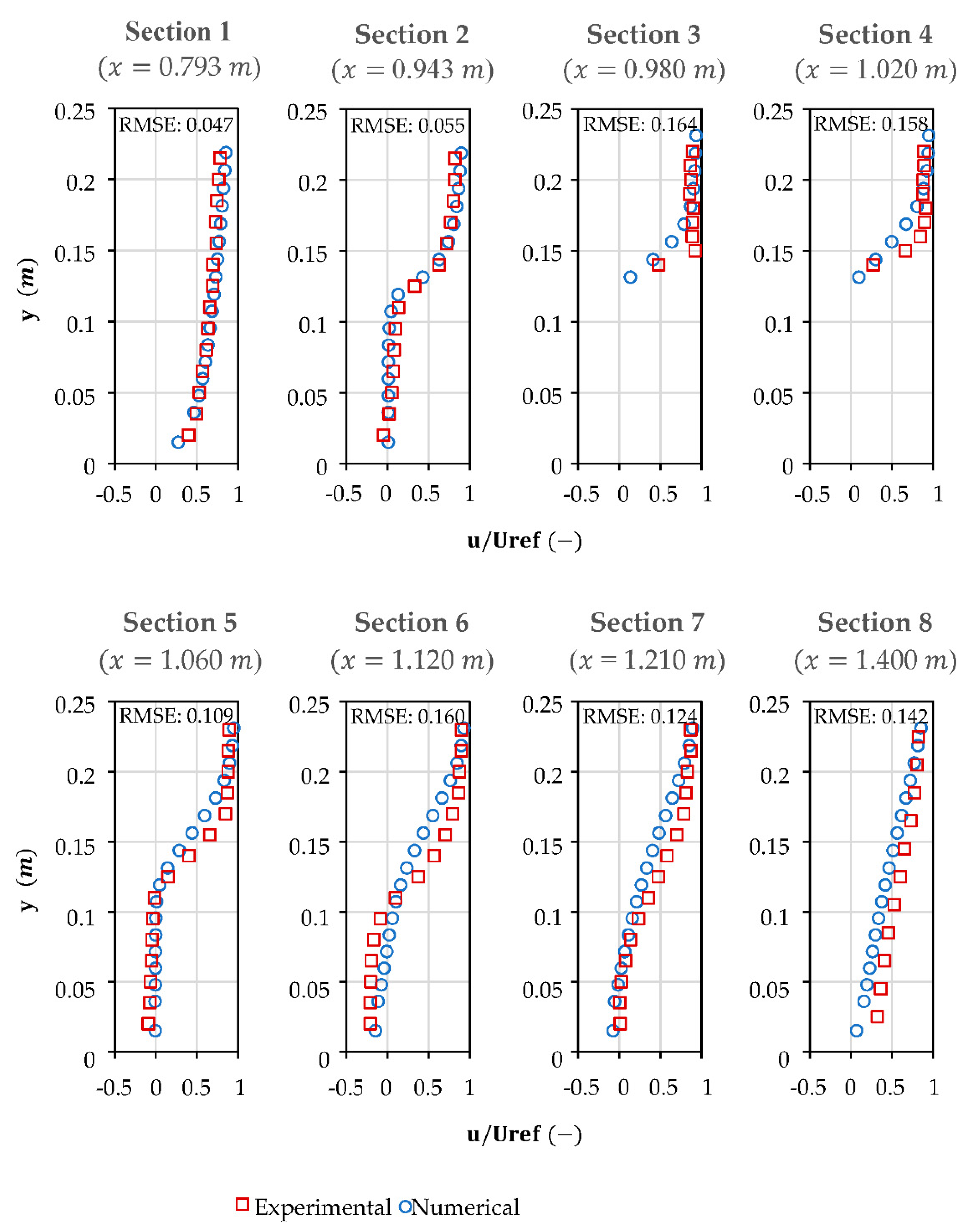
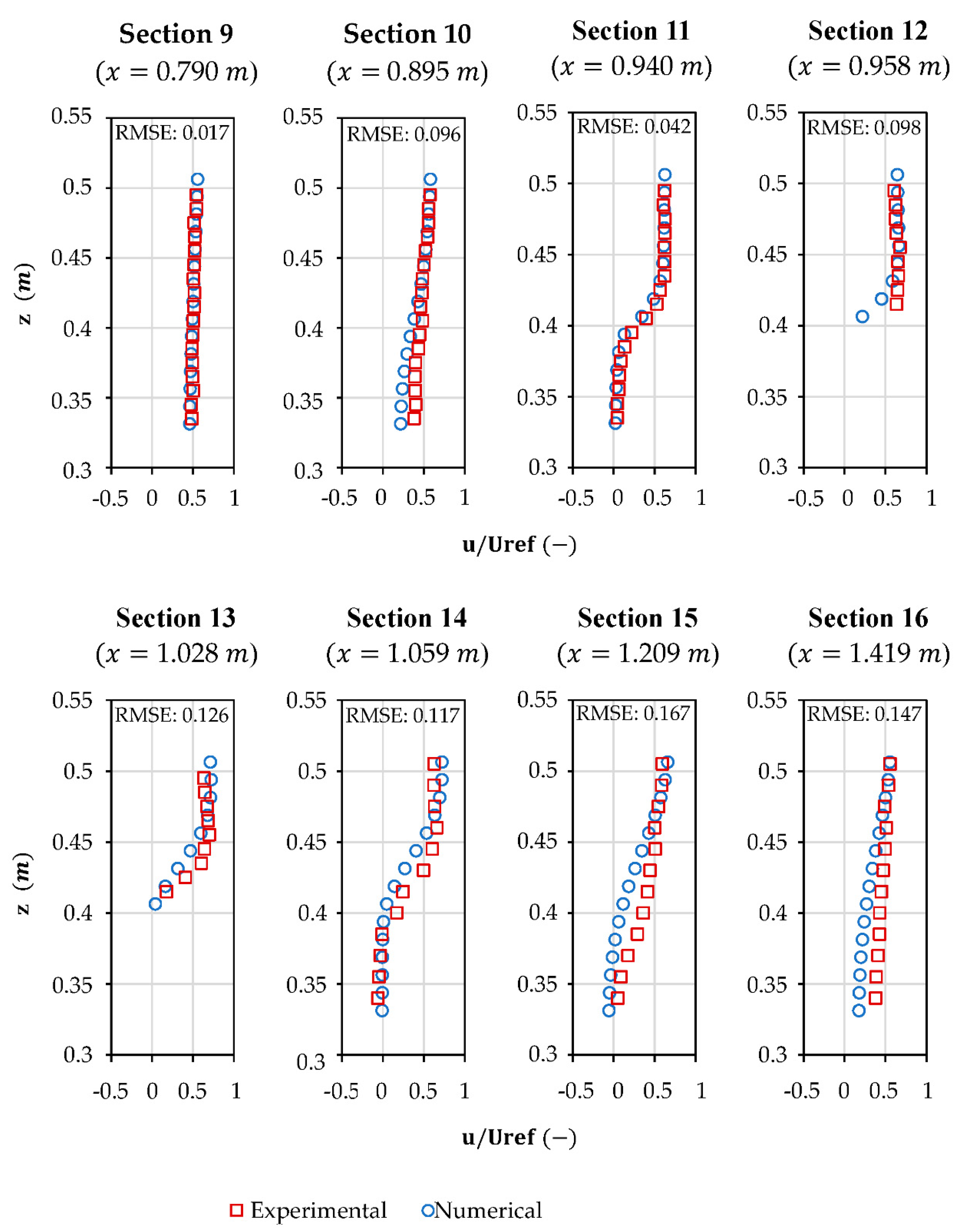
Appendix B. Model Validation

In order to validate the numerical model, the wind-tunnel measurements performed by Leitl and Schatzmann [28] in the meteorological institute of Hamburg university are compared with the numerical model predictions of the vertical and horizontal wind speed profiles in the vicinity of the building. The atmospheric boundary layer parameters are selected based on the values presented in Table A2, respectively. The total number of cells in the mesh is approximately 1.64 million, consisting of cells with the length, width and height almost equal to 0.0125 m . The results are then derived from sixteen different sections from which eight are located on the symmetry plane, z = 0.325 m , and the other eight a near-surface plane, y = 0.035 m , as shown in Figure A3. The comparisons and RMSE values presented in Figure A4 and Figure A5 show satisfactory agreements between the experimental data and the numerical model results. This shows the capability of the numerical model to predict both vertical and horizontal airflow patterns around the building.
Figure A3. Schematic representation of the vertical and horizontal measurement sections locating on the (a) symmetry plane, z = 0.325 m , and (b) a near-surface plane, y = 0.035 m .
Jmse 10 00013 g0a3
Figure A4. Comparisons between the wind-tunnel measurements performed by Leitl and Schatzmann [28] and the numerical model predictions of the vertical velocity profiles derived from eight different sections locating on the symmetry plane, z = 0.325 m .
Jmse 10 00013 g0a4
Figure A5. Comparisons between the wind-tunnel measurements performed by Leitl and Schatzmann [28] and the numerical model predictions of the horizontal velocity profiles derived from eight different sections locating on a near-surface plane, y =   0.035 m . The comparisons are performed for the right half side of the domain, where the building centreline and the lateral face of the building are located at z = 0.325 m and z = 0.400 m, respectively.
Jmse 10 00013 g0a5

References

  1. Marsh, G.P. The Earth as Modified by Human Action [A New Edition of Manand Nature]; Sampson Low, Marston, Low, and Searle: London, UK, 1874. [Google Scholar]
  2. Walker, H.J. Man’s impact on shorelines and nearshore environments: A geomorphological perspective. Geoforum 1984, 15, 395–417. [Google Scholar] [CrossRef]
  3. Nordstrom, K.F. Beaches and dunes of human-altered coasts. Prog. Phys. Geogr. 1994, 18, 497–516. [Google Scholar] [CrossRef]
  4. Jackson, N.L.; Nordstrom, K.F. Aeolian sediment transport and landforms in managed coastal systems: A review. Aeolian Res. 2011, 3, 181–196. [Google Scholar] [CrossRef]
  5. Walker, I.J.; Nickling, W.G. Dynamics of secondary airflow and sediment transport over and in the lee of transverse dunes. Prog. Phys. Geogr. 2002, 26, 47–75. [Google Scholar] [CrossRef]
  6. Nordstrom, K.F. Beaches and Dunes of Developed Coasts; Cambridge University Press: Cambridge, UK, 2004. [Google Scholar]
  7. Nordstrom, K.F.; McCluskey, J.M. The effects of houses and sand fences on the eolian sediment budget at Fire Island, New York. J. Coast. Res. 1985, 1, 39–46. [Google Scholar]
  8. Nordstrom, K.F.; McCluskey, J.M.; Rosen, P.S. Aeolian processes and dune characteristics of a developed shoreline. In Aeolian Geomorphology; Nickling, W.G., Ed.; Allen and Unwin: Boston, MA, USA, 1986; pp. 131–147. [Google Scholar]
  9. Fackrell, J.E. Parameters characterising dispersion in the near wake of buildings. J. Wind. Eng. Ind. Aerodyn. 1984, 16, 97–118. [Google Scholar] [CrossRef]
  10. Beranek, W.J. Wind Environment Around Single Buildings of Rectangular Shape; And, Wind Environment Around Building Configurations. In Stevin-Laboratory of the Department of Civil Engineering; Delft University of Technology: Delft, The Netherlands, 1984. [Google Scholar]
  11. Martinuzzi, R.; Tropea, C. The flow around surface-mounted, prismatic obstacles placed in a fully developed channel flow (data bank contribution). J. Fluids Eng. 1993, 115, 85–92. [Google Scholar] [CrossRef]
  12. Iversen, J.D.; Wang, W.P.; Rasmussen, K.R.; Mikkelsen, H.E.; Hasiuk, J.F.; Leach, R.N. The effect of a roughness element on local saltation transport. J. Wind. Eng. Ind. Aerodyn. 1990, 36, 845–854. [Google Scholar] [CrossRef]
  13. Iversen, J.D.; Wang, W.P.; Rasmussen, K.R.; Mikkelsen, H.E.; Leach, R.N. Roughness element effect on local and universal saltation transport. In Aeolian Grain Transport; Springer: Vienna, Austria, 1991; pp. 65–75. [Google Scholar]
  14. Tominaga, Y.; Okaze, T.; Mochida, A. Wind tunnel experiment and CFD analysis of sand erosion/deposition due to wind around an obstacle. J. Wind. Eng. Ind. Aerodyn. 2018, 182, 262–271. [Google Scholar] [CrossRef]
  15. Luo, W.; Dong, Z.; Qian, G.; Lu, J. Wind tunnel simulation of the three-dimensional airflow patterns behind cuboid obstacles at different angles of wind incidence, and their significance for the formation of sand shadows. Geomorphology 2012, 139, 258–270. [Google Scholar] [CrossRef]
  16. Sutton, S.L.F.; Neuman, C.M. Sediment entrainment to the lee of roughness elements: Effects of vortical structures. J. Geophys. Res. Earth Surf. 2008, 113, F2. [Google Scholar] [CrossRef] [Green Version]
  17. Beyers, M.; Waechter, B. Modeling transient snowdrift development around complex three-dimensional structures. J. Wind. Eng. Ind. Aerodyn. 2008, 96, 1603–1615. [Google Scholar] [CrossRef]
  18. Poppema, D.W.; Wijnberg, K.M.; Mulder, J.P.; Vos, S.E.; Hulscher, S.J. The effect of building geometry on the size of aeolian deposition patterns: Scale model experiments at the beach. Coast. Eng. 2021, 168, 103866. [Google Scholar] [CrossRef]
  19. Oke, T.R.; Mills, G.; Christen, A.; Voogt, J.A. Urban Climates; Cambridge University Press: Cambridge, UK, 2017. [Google Scholar]
  20. Peterka, J.A.; Meroney, R.N.; Kothari, K.M. Wind flow patterns about buildings. J. Wind. Eng. Ind. Aerodyn. 1985, 21, 21–38. [Google Scholar] [CrossRef]
  21. Blocken, B.; Stathopoulos, T.; Carmeliet, J.; Hensen, J.L. Application of computational fluid dynamics in building performance simulation for the outdoor environment: An overview. J. Build. Perform. Simul. 2011, 4, 157–184. [Google Scholar] [CrossRef]
  22. Hunt, J.C.R. The effect of single buildings and structures. Philos. Trans. R. Soc. Lond. Ser. A Math. Phys. Sci. 1971, 269, 457–467. [Google Scholar]
  23. Meroney, R.N. Turbulent Diffusion Near Buildings, Engineering Meteorology; CEP78-79RNM23; Colorado State University: Fort Collins, CO, USA, 1982. [Google Scholar]
  24. Meinders, E.R.; Hanjalic, K.; Martinuzzi, R.J. Experimental study of the local convection heat transfer from a wall-mounted cube in turbulent channel flow. J. Heat Transf. Trans ASME 1999, 121, 564–573. [Google Scholar] [CrossRef]
  25. Bitsuamlak, G.T.; Stathopoulos, T.; Bedard, C. Numerical evaluation of wind flow over complex terrain. J. Aerosp. Eng. 2004, 17, 135–145. [Google Scholar] [CrossRef]
  26. Smyth, T.A. A review of Computational Fluid Dynamics (CFD) airflow modelling over aeolian landforms. Aeolian Res. 2016, 22, 153–164. [Google Scholar] [CrossRef]
  27. Versteeg, H.K.; Malalasekera, W. An Introduction to Computational Fluid Dynamics: The Finite Volume Method; Pearson Education: London, UK, 2007. [Google Scholar]
  28. Leitl, B.; Schatzmann, M. Cedval at Hamburg University. 2010. Available online: http://www.mi.uni-hamburg.de/cedval (accessed on 1 December 2021).
  29. Bagnold, R.A. The movement of desert sand. Proc. R. Soc. Lond. Ser. A-Math. Phys. Sci. 1936, 157, 594–620. [Google Scholar] [CrossRef]
  30. O’brien, M.P.; Rindlaub, B.D. The transportation of sand by wind. Civ. Eng. 1936, 6, 325–327. [Google Scholar]
  31. Kawamura, R. Study on sand movement by wind. Rept. Inst. Sci. Technol. 1951, 5, 95–112. [Google Scholar]
  32. Zingg, A.W. Wind tunnel studies of the movement of sedimentary material. In Proceedings of the 5th Hydraulic Conference Bulletin; Inst. of Hydraulics Iowa City: Iowa City, IA, USA, 1953; Volume 34, pp. 111–135. [Google Scholar]
  33. Owen, P.R. Saltation or uniform grains in air. J. Fluid Mech. 1964, 20, 225–242. [Google Scholar] [CrossRef]
  34. Hsu, S.A. Wind stress criteria in eolian sand transport. J. Geophys. Res. 1971, 76, 8684–8686. [Google Scholar] [CrossRef]
  35. Iversen, J.D.; Greeley, R.; White, B.R.; Pollack, J.B. The effect of vertical distortion in the modeling of sedimentation phenomena: Martian crater wake streaks. J. Geophys. Res. 1976, 81, 4846–4856. [Google Scholar] [CrossRef]
  36. Maegley, W.J. Saltation and Martian sandstorms. Rev. Geophys. 1976, 14, 135–142. [Google Scholar] [CrossRef]
  37. Lettau, H.; Lettau, H.H. Experimental and micro-meteorological field studies of dune migration. In Exploring the World’s Driest Climate; IES Report; Leattau, H.H., Lettau, K., Eds.; University of Wisconsin: Madison, WI, USA, 1978; Volume 101, pp. 110–147. [Google Scholar]
  38. White, B.R. Soil transport by winds on Mars. J. Geophys. Res. Solid Earth 1979, 84, 4643–4651. [Google Scholar] [CrossRef]
  39. Delgado-Fernandez, I. A review of the application of the fetch effect to modelling sand supply to coastal foredunes. Aeolian Res. 2010, 2, 61–70. [Google Scholar] [CrossRef] [Green Version]
  40. Nolet, C.; Poortinga, A.; Roosjen, P.; Bartholomeus, H.; Ruessink, G. Measuring and modeling the effect of surface moisture on the spectral reflectance of coastal beach sand. PLoS ONE 2014, 9, e112151. [Google Scholar] [CrossRef]
  41. Hoonhout, B.; de Vries, S. Simulating spatiotemporal aeolian sediment supply at a mega nourishment. Coast. Eng. 2019, 145, 21–35. [Google Scholar] [CrossRef]
  42. McKenna Neuman, C.; Bédard, O. A wind tunnel study of flow structure adjustment on deformable sand beds containing a surface-mounted obstacle. J. Geophys. Res. Earth Surf. 2015, 120, 1824–1840. [Google Scholar] [CrossRef]
  43. Ferziger, J.H.; Perić, M.; Street, R.L. Computational Methods for Fluid Dynamics; Springer: Berlin/Heidelberg, Germany, 2002; Volume 3, pp. 196–200. [Google Scholar]
  44. Shapiro, A.H. Compressible Fluid Flow; Ronald Press: New York, NY, USA, 1953; p. 409. [Google Scholar]
  45. Moukalled, F.; Mangani, L.; Darwish, M. The Finite Volume Method in Computational Fluid Dynamics; Springer: Berlin/Heidelberg, Germany, 2016; Volume 6. [Google Scholar]
  46. Caretto, L.S.; Gosman, A.D.; Patankar, S.V.; Spalding, D.B. Two calculation procedures for steady, three-dimensional flows with recirculation. In Proceedings of the Third International Conference on Numerical Methods in Fluid Mechanics, Paris, France, 3–7 July 1972; pp. 60–68. [Google Scholar]
  47. Launder, B.E.; Spalding, D.B. The Numerical Computation of Turbulent Flows. Comput. Methods Appl. Mech. Eng. 1974, 3, 269–289. [Google Scholar] [CrossRef]
  48. Richards, P.J.; Hoxey, R.P. Appropriate boundary conditions for computational wind engineering models using the k-ε turbulence model. In Computational Wind Engineering 1; Elsevier: Amsterdam, The Netherlands, 1993; pp. 145–153. [Google Scholar]
  49. Launder, B.E.; Sharma, B.I. Application of the energy-dissipation model of turbulence to the calculation of flow near a spinning disc. Lett. Heat Mass Transf. 1974, 1, 131–137. [Google Scholar] [CrossRef]
  50. Blocken, B.; Stathopoulos, T.; Carmeliet, J. CFD simulation of the atmospheric boundary layer: Wall function problems. Atmos. Environ. 2007, 41, 238–252. [Google Scholar] [CrossRef]
  51. Bredberg, J. On the Wall Boundary Condition for Turbulence Models; Internal Report 00/4; Chalmers University of Technology, Department of Thermo and Fluid Dynamics: Goteborg, Sweden, 2000; pp. 8–16. [Google Scholar]
  52. Fluent, A.N.S.Y.S. ANSYS Fluent Theory Guide 15.0; ANSYS: Canonsburg, PA, USA, 2013; p. 33. [Google Scholar]
  53. Schlichting, H. Boundary Layer Theory; McGraw-Hill: New York, NY, USA, 1968; Volume 960. [Google Scholar]
  54. Tennekes, H.; Lumley, J.L. A First Course in Turbulence; The Massachusetts Institute of Technology Press: Cambridge, MA, USA, 1972. [Google Scholar]
  55. White, F.M. Viscous Fluid Flow; Mac Graw-Hill International Editions: New York, NY, USA, 1991. [Google Scholar]
  56. Liu, F. A Thorough Description of How Wall Functions Are Implemented in OpenFOAM; Nilsson, H., Ed.; Chalmers University of Technology: Göteborg, Sweden, 2016; Available online: http://www.tfd.chalmers.se/~hani/kurser/OS_CFD (accessed on 1 December 2021).
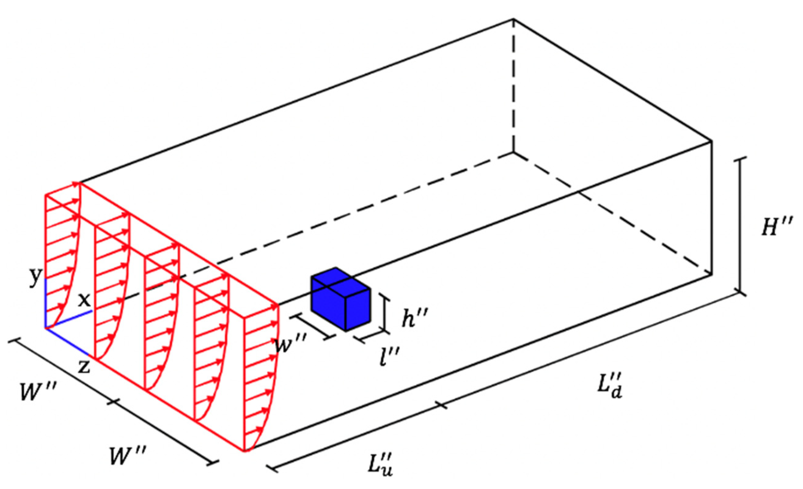
Figure 1. Buildings at beach–dune interface on the (a) Egmond beach, and (b) Zandvoort beach (https://www.hollandluchtfoto.nl (accessed on 1 December 2021)), The Netherlands.
Jmse 10 00013 g001
Figure 2. Morphological loop indicating the interactions between buildings at the beach, airflow patterns, sediment transport and bed morphology.
Jmse 10 00013 g002
Figure 3. Schematic airflow patterns around an isolated cubical building with wind incidence angle perpendicular to the building (a) windward view, and (b) leeward view (modified from Oke et al. [19] and Blocken et al. [21]).
Jmse 10 00013 g003
Figure 4. Schematic configuration of the computational domain and the surface-mounted building.
Jmse 10 00013 g004
Figure 5. The impact of building length on (ae) wind velocity magnitude (color) and direction (streamlines), (f) length of the downwind recirculation region, L d , just behind the leeward face of the building along the centerline, (g) wind velocity magnitude downstream of the building after flow reattachment along the centerline, and (h) streamwise, u, and vertical wind velocity components, v, upstream of the building along the centerline. Results are derived for a horizontal near-surface plane, y = 0.0125 m . The building width and height are w 0 and h 0 , respectively. The building length, l , is varied as l 0 , 1.5 l 0 , 2 l 0 , 2.5 l 0 , and 3 l 0 .
Jmse 10 00013 g005
Figure 6. The impact of building width on (ae) wind velocity magnitude (color) and direction (streamlines), (f) length of the downwind recirculation region, L d , just behind the leeward face of the building along the centerline, (g) wind velocity magnitude downstream of the building after flow reattachment along the centerline, and (h) streamwise, u, and vertical wind velocity components, v, upstream of the building along the centerline. Results are derived for a horizontal near-surface plane, y = 0.0125 m . The building length and height are l 0 and h 0 , respectively. The building width, w , is varied as w 0 , 1.5 w 0 , 2 w 0 , 2.5 w 0 , and 3 w 0 .
Jmse 10 00013 g006
Figure 7. The impact of building height on (ae) wind velocity magnitude (color) and direction (streamlines), (f) length of the downwind recirculation region, L d , just behind the leeward face of the building along the centerline, (g) wind velocity magnitude downstream of the building after flow reattachment along the centerline, and (h) wind velocity magnitude, streamwise, u, and vertical velocity components, v, upstream of the building along the centerline. Results are derived for a horizontal near-surface plane, y =   0.0125 m . The building length and width are l 0 and w 0 , respectively. The building height, h , is varied as h 0 , 1.5 h 0 , 2 h 0 , 2.5 h 0 , and 3 h 0 .
Jmse 10 00013 g007
Figure 8. Numerical model predictions of the erosion and deposition patterns inferred from the convergence of the third-order horizontal wind velocity field at a horizontal near-surface plane, (a) y =   0.25 m for the full-scale building, and (b) y =   0.015 m for the small-scale building. The wind direction is from the left and perpendicular to the front face of the buildings. The white lines are zero contours.
Jmse 10 00013 g008
Figure 9. Field observations of erosion and deposition patterns around a (ad) full-scale model at Noordwijk beach, and (e,f) small-scale models at De Zandmotor beach, the Netherlands. The arrows show the wind directions. (c,e,f were obtained from Poppema et al. [18]).
Jmse 10 00013 g009
Figure 10. The impact of building length on erosion and deposition patterns inferred from the convergence of the third-order horizontal wind velocity field at a near-surface plane,   y =   0.0125 m . The building width and height are w 0 and h 0 , respectively. The building length, l , is varied as (a) l 0 , (b) 1.5 l 0 , (c) 2 l 0 , (d) 2.5 l 0 , and (e) 3 l 0 .
Jmse 10 00013 g010
Figure 11. The Impact of building width on erosion and deposition patterns inferred from the convergence of the third-order horizontal wind velocity field at a near-surface plane, y =   0.0125 m . The building length and height are l 0 and h 0 , respectively. The building width, w , is varied as (a) w 0 , (b) 1.5 w 0 , (c) 2 w 0 , (d) 2.5 w 0 , and (e) 3 w 0 .
Jmse 10 00013 g011
Figure 12. The Impact of building height on erosion and deposition patterns inferred from the convergence of the third-order horizontal wind velocity field at a near-surface plane, y = 0.0125 m . The building length and width are l 0 and w 0 , respectively. The building height, h , is varied as h 0 , 1.5 h 0 , 2 h 0 , 2.5 h 0 , and 3 h 0 .
Jmse 10 00013 g012
Figure 13. Numerical model predictions of the erosion and deposition patterns inferred from the convergence of the third-order horizontal wind velocity field at a horizontal near-surface plane, y = 0.25 m , around the full-scale building. The reference wind velocity magnitude is 17   m / s at a reference height of 1.8   m . The wind direction is from the left and perpendicular to the front face of the building. The white lines are zero contours.
Jmse 10 00013 g013
Table 1. Definition and values of the geometric parameters of the computational domain and the surface-mounted building.
ParameterDefinition
L u Upstream distance between the domain inlet and the building centerline
L d Downstream distance between the domain outlet and the building centerline
W Lateral distance between the lateral sides of the domain and the building centerline
H Height of the domain
l Length of the building
w Width of the building
h Height of the building
Table 2. An overview of the conducted simulations and the building dimensions in each case. The length, width and height of the computational domain is 3   m , 2   m and 1.5   m , respectively.
Simulation ID Building   Length   ( l )   [ m ] Building   Width   ( w )   [ m ] Building   Height   ( h )   [ m ]
Reference building
l 0 × w 0 × h 0 0.10000.15000.1250
Impact of building length
1.5 l 0 × w 0 × h 0 0.15000.15000.1250
2 l 0 × w 0 × h 0 0.20000.15000.1250
2.5 l 0 × w 0 × h 0 0.25000.15000.1250
3 l 0 × w 0 × h 0 0.30000.15000.1250
Impact of building width
l 0 × 1.5 w 0 × h 0 0.10000.22500.1250
l 0 × 2 w 0 × h 0 0.10000.30000.1250
l 0 × 2.5 w 0 × h 0 0.10000.37500.1250
l 0 × 3 w 0 × h 0 0.10000.45000.1250
Impact of building height
l 0 × w 0 × 1.5 h 0 0.10000.15000.1875
l 0 × w 0 × 2 h 0 0.10000.15000.2500
l 0 × w 0 × 2.5 h 0 0.10000.15000.3125
l 0 × w 0 × 3 h 0 0.10000.15000.3750
Publisher’s Note: MDPI stays neutral with regard to jurisdictional claims in published maps and institutional affiliations.

