Promoting Agricultural Green Productivity Through Geographical Indication Certification: Mechanisms and Spatial Heterogeneity

Abstract

Agricultural green transformation is important for achieving economic growth and environmental sustainability. Geographical indication agricultural products (GIAPs) have become a useful tool for improving agricultural green total factor productivity (AGTFP). However, the mechanisms through which GIAPs affect AGTFP and their spatial differences are not yet fully understood. This study uses a balanced panel of 290 Chinese cities from 2008 to 2024 and combines Double Machine Learning (DML), Geographically Weighted Random Forest (GWRF), and Shapley Additive explanations (SHAP) to examine the effects of GIAPs on AGTFP. The results show that GIAPs significantly enhance AGTFP, primarily through agricultural industry agglomeration and the downstream penetration of leading agricultural enterprises. The effects exhibit substantial spatial and category heterogeneity. GWRF-SHAP results further reveal a clear geographical gradient, with GIAPs exhibiting greater predictive importance and contribution in inland than coastal regions. These findings highlight the need for region- and product-specific strategies to leverage GIAPs for agricultural green transformation. This study provides new evidence on the green development effects of geographical indications and offers policy insights for promoting sustainable agricultural development.

1. Introduction

Agricultural green total factor productivity (AGTFP) has emerged as a critical indicator of the quality of agricultural economic growth, resource-use efficiency, and the compatibility between agricultural production and environmental sustainability. It is also fundamental to advancing the green transformation and modernization of agriculture [1]. Yet, conventional agricultural development has long relied on input-intensive and resource-consuming production practices. Although these practices have supported substantial gains in agricultural output, they have also generated mounting environmental pressures, including excessive resource depletion, agricultural non-point-source pollution, and ecosystem degradation [2]. As one of the world’s largest agricultural producers, China faces particularly acute challenges: the agricultural sector accounts for approximately 17% of the country’s greenhouse-gas emissions, underscoring the urgency of accelerating the transition towards greener agricultural production [3]. Against this backdrop, geographical indication agricultural products (GIAPs) represent an institutional arrangement that integrates place-based resource endowments, distinctive product attributes, and intellectual property protection. GIAPs cover many types of agricultural products, including fruits, tea, livestock and poultry, aquatic products, and medicinal herbs. GIAPs can use local production conditions, quality certification, and brand premiums to increase agricultural value added and improve regional competitiveness [4]. More importantly, these factors may encourage producers to use more standardized and environmentally sustainable production practices. This makes GIAPs a useful tool for promoting high-quality agricultural development [5]. This potential has also gained increasing policy recognition. China’s 2025 Central No. 1 Document called for the vigorous development of green and distinctive agricultural products, while at the international level, the European Union has advocated expanding the protection of geographical indications within the World Trade Organization (WTO) framework as part of broader efforts to promote sustainable agriculture [6]. These developments highlight the growing strategic relevance of GIAPs in the global transition towards greener agricultural systems. Despite this policy momentum, whether GIAPs can effectively reconcile agricultural economic development with environmental sustainability and, ultimately, generate sustained improvements in AGTFP remains an empirical question. Moreover, substantial spatial differences in resource endowments, production conditions, and institutional environments imply that the benefits of GIAPs may not be uniform across regions. Identifying how the place-based institutional advantages of GIAPs can be effectively leveraged under different regional conditions, and through which pathways they can enhance AGTFP, is therefore essential for advancing agricultural modernization and designing context-sensitive strategies for green agricultural transformation.

Compared with conventional productivity measures, AGTFP considers resource constraints and environmental impacts in agricultural production. It considers both desirable and undesirable outputs, so it provides a more complete measure of the quality and sustainability of agricultural development [7]. Existing methods for measuring AGTFP mainly include parametric estimation based on stochastic frontier analysis (SFA) [8] and non-parametric estimation based on data envelopment analysis (DEA) [9]. As green agriculture has developed, AGTFP has become an important measure of high-quality agricultural development. Many studies have examined its main factors, including green finance [10], environmental regulation [1], and green technological innovation in agriculture [11]. These studies mainly focus on how institutions and policies affect green agricultural development. In comparison, studies on GIAPs have mainly focused on their economic effects. Existing studies show that GIAPs have clear spatial clustering. Both European and Chinese markets show a similar pattern, with more GIAPs in coastal areas and fewer in inland areas [12]. GIAPs can increase agricultural output value and local fiscal revenues through brand premiums, quality certification, and market incentives [13]. They can also improve the ability of agricultural industries to deal with economic and environmental shocks [4].

Existing research has mainly focused on the economic value of GIAPs, while their role in green development has received less attention. As agricultural intellectual property that combines place-based identity with brand value [4,14], GIAPs can increase the returns to agricultural producers and facilitate the industrialization of distinctive agricultural sectors by strengthening product differentiation, enhancing market recognition, and fostering industrial integration [5]. Yet the ultimate objective of agricultural green transformation extends beyond increasing economic output; it requires a coordinated improvement in resource-use efficiency, a reduction in environmental pressures, and the creation of ecological value [1,15]. Whether GIAPs can transcend traditional market value-added functions by transforming agricultural production methods and resource allocation models to enhance AGTFP remains a topic that lacks sufficient discussion. Importantly, the relationship between GIAPs and AGTFP may not be adequately characterized by a simple linear process. The magnitude and direction of their effects may depend on agricultural organizational structures, technological diffusion capacity, and broader regional development conditions [16]. Moreover, substantial spatial disparities in natural resource endowments, agricultural development foundations, marketization, and environmental constraints may lead to pronounced regional heterogeneity in the extent to which GIAPs generate green value [17]. Understanding these nonlinear and spatially differentiated effects is therefore crucial for determining when and where GIAPs can effectively contribute to agricultural green transformation.

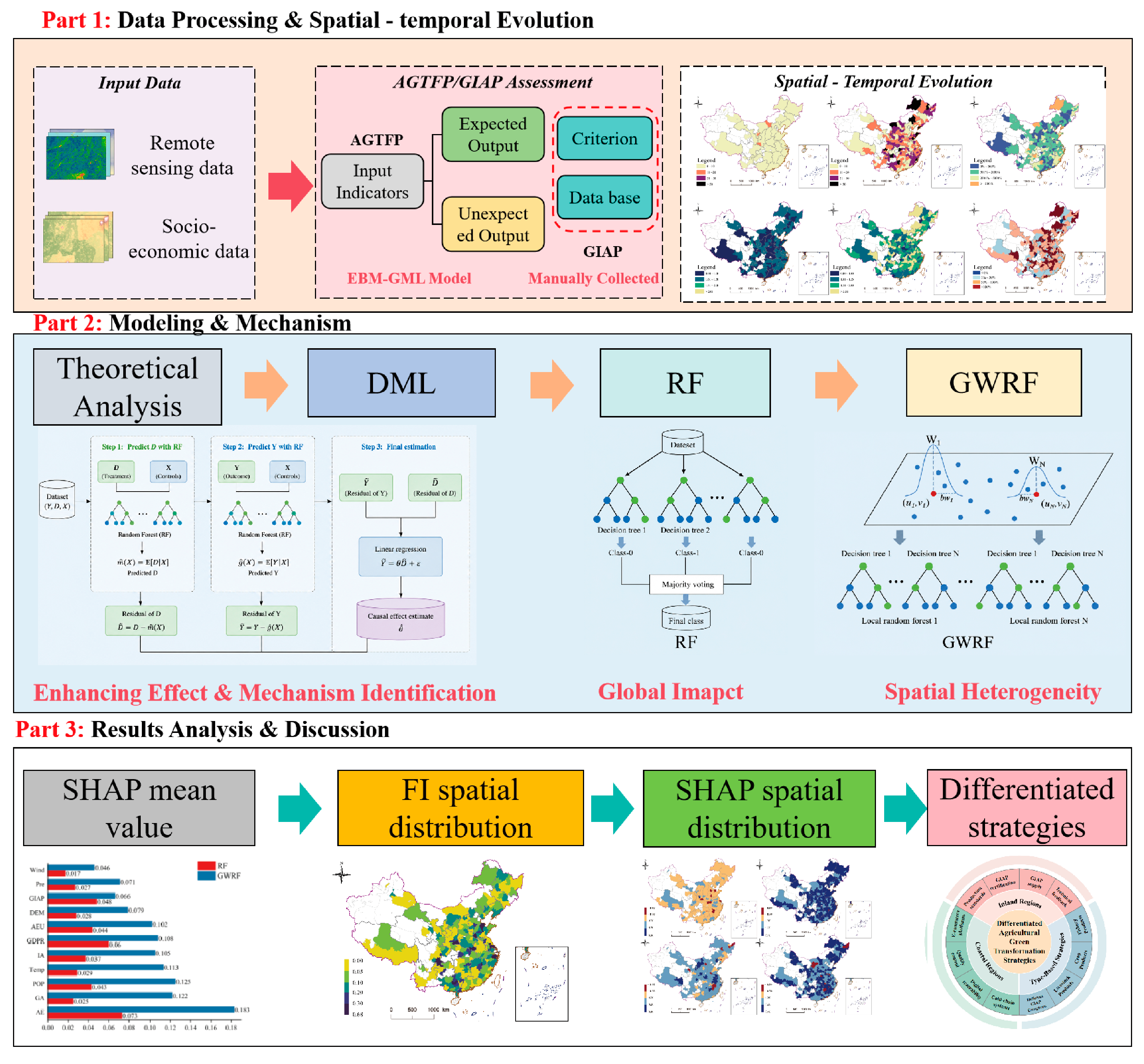
Clarifying the mechanisms linking GIAPs to AGTFP has broader implications beyond the Chinese context. It can inform strategies for upgrading distinctive agricultural products, while also contributing to the broader challenge of reducing the environmental footprint of agriculture and accelerating the transition towards sustainable food systems. To address the above research gaps, we integrate multi-source data, rigorous productivity measurement, causal machine learning, and spatially interpretable machine learning into a unified analytical framework. First, we assemble a comprehensive dataset combining remote-sensing information with socioeconomic statistics. We then develop a rigorous measurement framework in which city-level AGTFP is estimated using an EBM-GML model, which addresses several limitations associated with the conventional super-efficiency Slack-Based Measure (SBM) approach [18]. GIAP development is measured by the cumulative number of officially certified GIAPs in each city, manually compiled from certification announcements. Second, we combine machine learning with causal inference to identify the effects and potential mechanisms of GIAPs. Specifically, a random forest (RF) model embedded within a double machine learning (DML) framework is employed to estimate the enhancing effect of GIAPs on AGTFP. Third, to uncover spatially differentiated effects, we employ geographically weighted random forest (GWRF) together with Shapley Additive Explanations (SHAP) to quantify the relative explanatory contributions of GIAPs and other covariates and to characterize their spatial heterogeneity. We further examine whether these effects differ across major GIAP categories. Finally, based on the empirical evidence, we develop spatially differentiated strategies for transforming urban agricultural development, with the aim of enhancing AGTFP and accelerating agricultural green transformation. The overall analytical framework is presented in Figure 1.

This study makes three contributions. First, it provides robust quantitative evidence on the role of GIAPs in advancing AGTFP. Using a large-scale city-level panel dataset, we extend existing research that has largely focused on provincial-level evidence [19,20], revealing the mechanisms and spatially differentiated patterns underlying the GIAP and AGTFP relationship. Second, we develop an integrated causal–spatial machine learning framework that combines DML with GWRF-SHAP. While DML is effective in identifying causal effects in the presence of high-dimensional confounding, it may overlook spatial heterogeneity; conversely, GWRF-SHAP captures spatially varying relationships but provides limited evidence on causal mechanisms. Previous studies have employed individual methods—DML, RF, and GWRF—to explore the relationship between agriculture and green transition [21,22]. By integrating these approaches, we are now able to conduct a more comprehensive assessment of the causal effects of GIAPs on AGTFP, its spatial heterogeneity, and its underlying mechanisms of action. Third, from a policy perspective, whereas previous studies have largely provided broad and uniform guidance for agricultural green transformation [23], our findings offer more targeted implications for developing place-based and differentiated GIAP strategies. By accounting for regional heterogeneity, the evidence can inform differentiated national strategies for GIAP development and provide a scientific basis for advancing the sustainable development of distinctive agricultural systems globally.

2. Theoretical Analysis

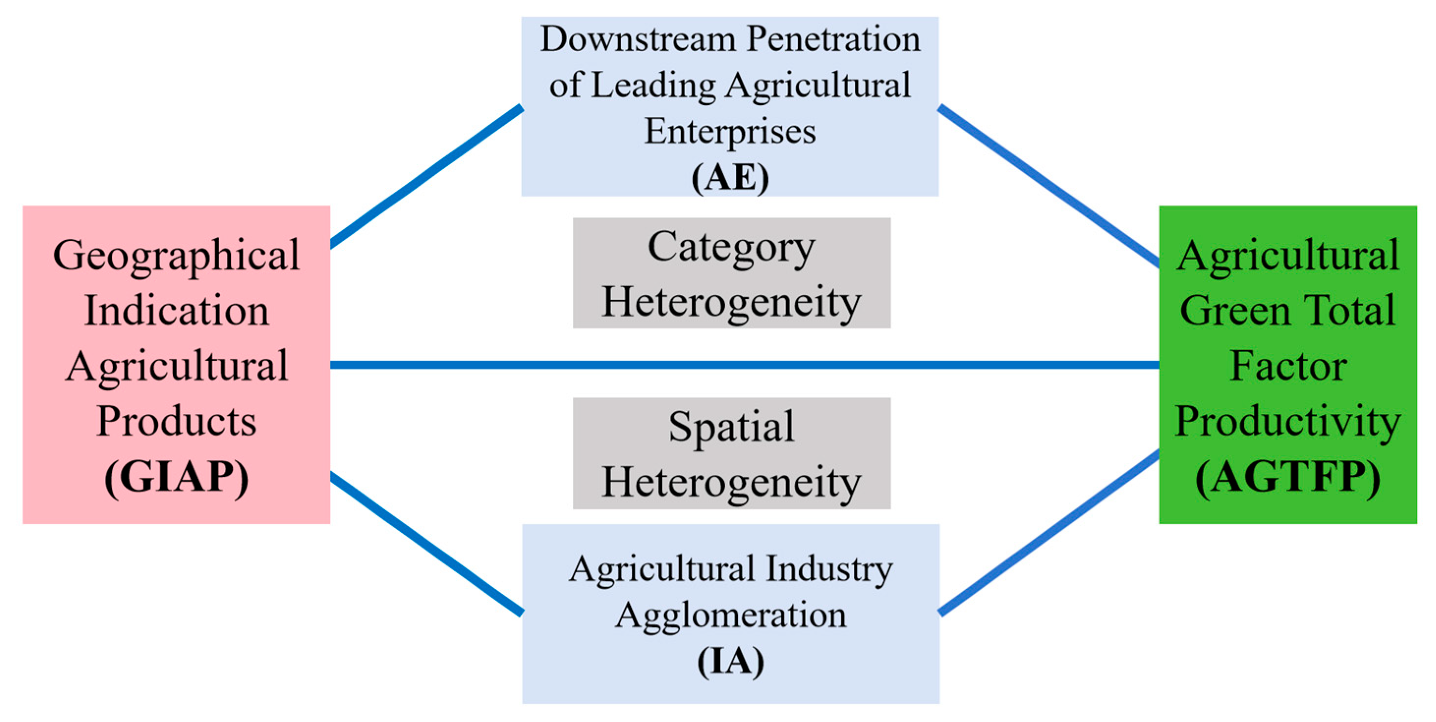
Amid the accelerating global transition towards green agriculture, GIAPs have emerged as an important institutional instrument for directing agricultural resources towards low-carbon and environmentally sustainable production. By reshaping producers’ incentives, production practices, and resource-allocation decisions, GIAPs may exert substantial effects on AGTFP. Building on this premise, we develop a theoretical framework to explain how GIAPs can enhance AGTFP through direct and indirect mechanisms (Figure 2).

2.1. The Direct Effect

AGTFP captures the capacity of agricultural production to generate economic output while simultaneously improving resource efficiency and environmental performance. It reflects a production process characterized by resource conservation, environmental sustainability, and ecological coordination, in which technological progress and more efficient factor allocation jointly contribute to improvements in both agricultural productivity and ecological outcomes [24,25].

From the perspective of property-rights theory, clearly defined and effectively enforced property rights strengthen producers’ expectations regarding the returns from resource use and long-term asset value, thereby creating incentives to preserve resource quality and improve resource-use efficiency [26]. GIAPs represent a form of agricultural intellectual property characterized by place specificity and exclusive legal protection. By linking the natural and ecological attributes of a particular geographical area with product quality and market reputation, GIAPs effectively transform place-based ecological conditions and product characteristics into economically valuable property rights. Unlike conventional agricultural products, GIAPs typically command stronger brand recognition and market premiums. Producers therefore have greater incentives to protect the reputation of the geographical indication and secure its long-term economic value, creating an institutional alignment between economic returns and environmental stewardship [27].

This incentive operates through two closely related channels. First, GIAP certification is typically accompanied by explicit production standards, quality requirements, and traceability mechanisms. These institutional constraints strengthen quality control and property-rights protection, encouraging producers to optimize the allocation of land, labor, capital, and other productive inputs. By reducing excessive reliance on chemical fertilizers, pesticides, and other external inputs, GIAPs can improve agricultural resource-use efficiency and reduce the environmental costs of production [28,29]. Second, the quality and market value of GIAPs are closely tied to the ecological conditions of their places of origin. Environmental degradation can therefore undermine product quality, market reputation, and the economic value of the geographical indication. Producers consequently have stronger incentives to adopt green technologies and environmentally friendly production practices to preserve product quality and protect brand value [30,31]. Therefore, GIAPs establish a direct economic linkage between ecological quality and market returns. This linkage strengthens producers’ incentives to adopt long-term green production practices, shifts agricultural production away from extensive input-driven growth towards resource-efficient and environmentally sustainable modes of production, and ultimately enhances AGTFP.

2.2. The Indirect Effect

GIAPs may enhance AGTFP through two complementary organizational channels. The first operates through agricultural industrial agglomeration. According to Marshallian agglomeration theory, the spatial concentration of producers generates external economies through specialization, shared intermediate inputs, and knowledge and technological spillovers, thereby improving regional productivity [32]. By leveraging place-specific natural and cultural endowments to generate brand premiums, GIAPs increase the market attractiveness of distinctive agricultural products and encourage the concentration of capital, labor, technology, and other productive factors in areas with comparative advantages [33,34]. As producers and supporting industries become increasingly concentrated, the conditions for coordinated green production also improve. On the one hand, industrial agglomeration strengthens spatial interactions among producers, facilitating the coordinated adoption of green production standards and environmental regulations and enabling producers to share environmental infrastructure, thereby reducing the unit cost of pollution control. On the other hand, the knowledge spillovers and technological diffusion generated by agglomeration accelerate the dissemination of green production technologies among local producers and reduce the costs associated with accessing and adopting such technologies [35]. This facilitates the diffusion and application of green innovations throughout the production area. Thus, the agglomeration effects generated by GIAPs can improve agricultural resource allocation and environmental performance by lowering the costs of environmental governance and strengthening green knowledge and technology spillovers, ultimately contributing to higher AGTFP.

The second mechanism operates through the downstream penetration of leading agricultural enterprises. Transaction cost theory suggests that when agricultural producers are highly fragmented and market transactions are characterized by information asymmetries, weak quality monitoring, and high coordination costs, firms can improve value-chain efficiency through vertical integration and organized production, thereby reducing search, bargaining, monitoring, and quality-control costs. As important organizational intermediaries connecting smallholders with modern agriculture, leading agricultural enterprises play a critical role in introducing technologies, establishing production standards, and expanding market access [36,37]. The regional brand value and relatively stable market demand created by GIAPs can reduce the uncertainty associated with entering distinctive agricultural production areas, thereby providing persistent economic incentives for leading firms to extend their operations into producing regions and rural counties.

Leading agricultural enterprises also possess stronger capabilities in technological innovation, standard setting, and resource integration. Through organized production, they can reduce the costs of green technology diffusion and quality monitoring [38], while encouraging surrounding farmers and cooperatives to adopt cleaner production practices, precision fertilization, and environmentally friendly pest and disease management. More importantly, firms can use GIAP production standards as an organizational link through which environmental requirements are embedded across production, processing, and distribution stages. By establishing traceability systems and green supply-chain management practices, and by using contract farming and other benefit-sharing arrangements, leading firms can transmit these standards to dispersed smallholders [39,40]. In this way, the branding and standardization advantages of GIAPs can be translated through the organizational capacity of leading firms from product certification into transformation of production practices. By reducing transaction costs while facilitating the diffusion of green technologies and production standards to the agricultural production frontier, this mechanism can promote the broader greening of production systems and ultimately create favorable conditions for improving AGTFP.

2.3. Spatial and Category Heterogeneity Effect

Although GIAPs have the potential to facilitate agricultural green transformation, their effects on AGTFP are unlikely to be uniform across regions or product categories. From a spatial heterogeneity perspective, regions differ substantially in their natural resource endowments, agricultural development foundations, degree of marketization, and capacity for industrial organization [17]. These differences can shape both the value-realization pathways of GIAPs and their capacity to generate green productivity gains. On the one hand, regions endowed with abundant ecological resources and well-established distinctive agricultural sectors may be better positioned to integrate GIAPs with local industrial development. Through brand building, industrial agglomeration, and value-chain extension, GIAPs in these regions can more readily translate place-based advantages into improvements in agricultural green development. On the other hand, economically advanced regions typically possess more developed markets, infrastructure, and industrial systems, which may strengthen the commercialization potential of GIAPs. However, their agricultural green transformation may also face tighter resource and environmental constraints [1] and increasingly depend on technological upgrading [41], potentially altering the marginal contribution of GIAPs to AGTFP.

Heterogeneity may also arise across GIAP categories because different products differ in their production technologies, dependence on natural resources, and value-chain structures. For example, crop-based GIAPs are closely linked to land resources, ecological conditions, and green cultivation technologies; their contribution to AGTFP is therefore more likely to operate through improvements in production practices and resource-use efficiency. Livestock-related GIAPs may place greater reliance on value chain integration, processing capabilities, and the realization of brand value, making organizational coordination and downstream value creation particularly critical. Fishery-related GIAPs, in contrast, are more directly constrained by aquatic ecosystems and the sustainable use of water resources, implying green transformation pathways that differ fundamentally from those of land-based agriculture. Thus, the effects of GIAPs on AGTFP are shaped not only by the existence of certification itself, but also by the interaction between place-specific conditions and product-specific characteristics. Identifying these spatial and product-type differences is therefore essential for understanding where GIAPs are most effective, through which context-dependent pathways they operate, and how agricultural green transformation strategies can be tailored to different regional and product settings.

3. Research Design

3.1. Study Area

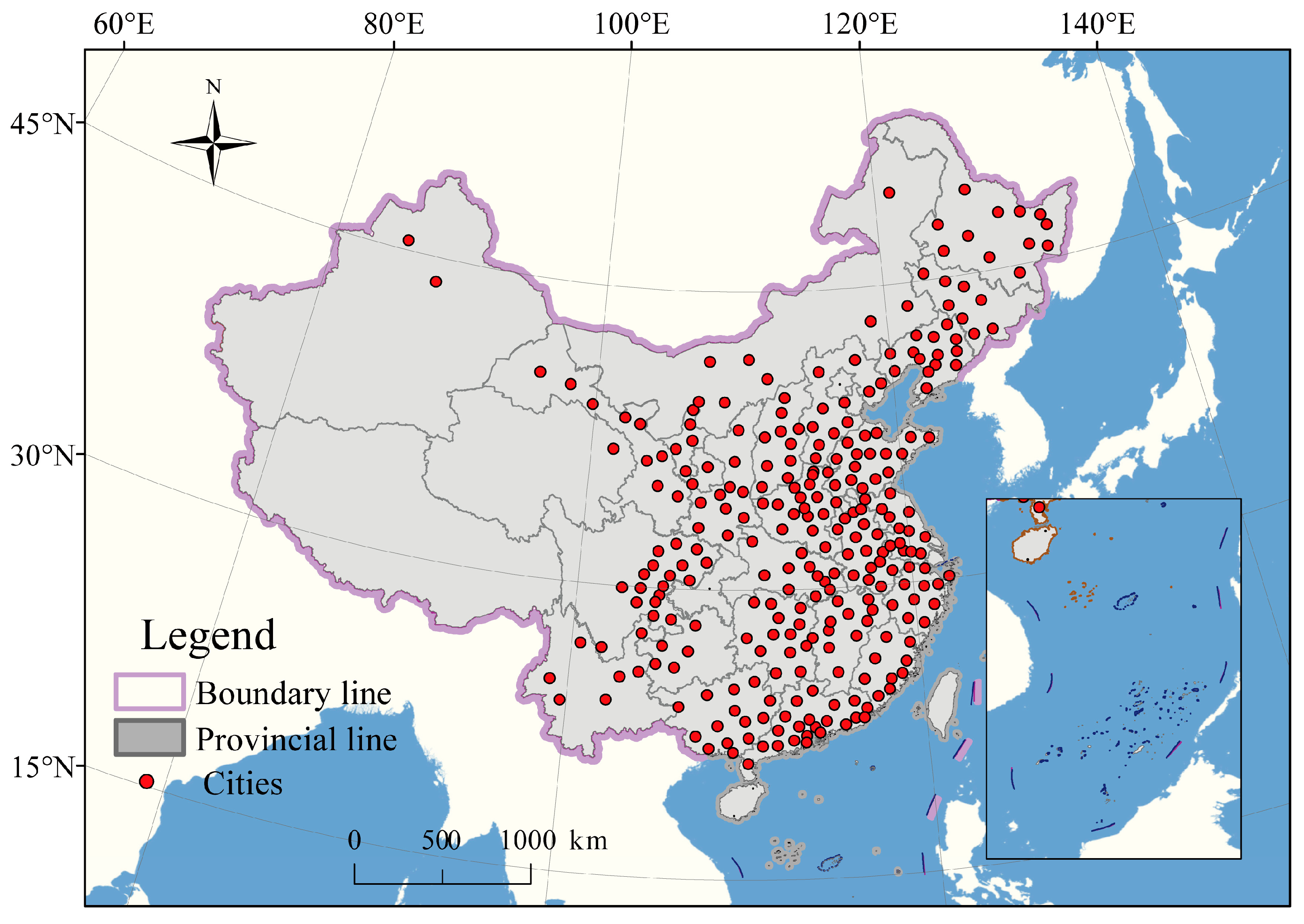
After matching the socio-economic data with remote sensing data, we excluded urban samples with missing AGTFP, GIAPs, or control variable data; as a result, we selected 290 cities across China (2008–2024) as the study sample (Figure 3). During the study period, no administrative boundary changes occurred among these cities; the complete list of cities is provided in the Supplementary Materials.

3.2. Methods

3.2.1. DML

The Double Machine Learning (DML) method effectively mitigates overfitting bias in scenarios involving high-dimensional confounding factors by combining machine learning with orthogonalization techniques [42]; the baseline model is defined as follows:

AGTFP_it = α₀GIAP_it + f(X_it) + ε_it

(1)

E(ε_it|GIAP_it,X_it) = 0

(2)

where i denotes the city, t denotes time; AGTFP_it represents the dependent variable; GIAP_it is the treatment variable; α₀ is used to capture the target parameter; X_it is the vector of control variables; and ε_it represents the random error term, with conditional mean equal to 0.

GIAP_it = g(X_it) + μ_it

(3)

E(μ_it|X_it) = 0

(4)

Based on the orthogonalization principle of the Frisch–Wage–Lovell theorem, this paper employs machine learning methods to estimate the disturbance function g(X_it), and the outcome function f(X_it), g(X_it) eliminates the influence of high-dimensional control variables X_it and obtains the residual ${\widehat{\mu }}_{\mathit{it}}={\mathit{GIAP}}_{\mathit{it}}-\widehat{g}\left(X_{\mathit{it}}\right)$. This residualization step is part of the orthogonalization procedure in DML rather than an instrumental-variable procedure. The residual term is used to estimate the treatment variable coefficient α₀.

$${\widehat{\alpha }}_0={\left({\displaystyle \frac{1}{n}}\sum _{i\in I,t\in T} {\widehat{\mu }}_{\mathit{it}}{\mathit{GIAP}}_{\mathit{it}}\right)}^{-1}{\displaystyle \frac{1}{n}}\sum _{i\in I,t\in T} {\widehat{\mu }}_{\mathit{it}}\left[{\mathit{AGTFP}}_{\mathit{it}}-\right.\left.\widehat{f}\left(X_{\mathit{it}}\right)\right]$$

(5)

To mitigate overfitting and improve the reliability of the machine learning estimation, we randomly divide the full sample into a model-development subsample (80%) and an independent assessment subsample (20%). This 80/20 split is used for model development and assessment and does not determine the final DML estimation sample. Within the model-development subsample, five-fold cross-fitting is conducted to estimate the nuisance functions for the outcome and treatment equations. Specifically, in each iteration, four folds are used to train the Random Forest models, while the remaining fold is used to generate out-of-fold predictions. These predictions are then used to construct the residualized outcome and treatment variables for the orthogonalized DML estimation. The final treatment effect is estimated using the full sample. City and year fixed effects are included to account for time-invariant city-specific characteristics and common year shocks. Standard errors are clustered at the city level to account for within-city dependence over time.

3.2.2. Random Forest

The Random Forest (RF) is an ensemble learning-based machine learning method that performs classification and regression prediction by combining multiple Decision Trees (DTs) [43]. Its fundamental workflow consists of the following steps: First, bootstrap sampling with replacement is applied to the training samples to generate multiple subsamples; next, features are randomly selected to construct individual decision trees, and the predictions from these trees are then aggregated to produce the final output. Each tree is typically trained using a certain number of samples, while the remaining samples constitute the Out-of-Bag (OOB) set. The OOB error is used to evaluate the relative contribution of each variable to the prediction results, and based on this evaluation, variable importance metrics are calculated according to the following formula:

$$F{I}_x={\displaystyle \frac{1}{n}}{\sum }_t\left(\mathit{OO}{B}_{\mathit{MSE},{\mathit{perm}}_x}^t-\mathit{OO}{B}_{\mathit{MSE}}^t\right)$$

(6)

where FI_x denotes the importance of the influence factor x; n represents the number of decision trees in the random forest; while $\mathit{OO}{B}_{\mathit{MSE}}^t$ and $\mathit{OO}{B}_{\mathit{MSE},{\mathrm{perm}}_x}^t$ represent the mean squared error before and after permuting decision tree t, respectively. By integrating multiple decision trees, the random forest effectively reduces the overfitting risk associated with individual models and exhibits strong robustness against noise and outliers. This study constructs a random forest model using the ‘randomForest’ package (version 4.7-1.1) in R 4.2.2 [14].

3.2.3. Geographically Weighted Random Forest

Random Forest (RF) has certain limitations; its assumed global model structure cannot capture the spatial consistency among variable relationships, making it difficult to characterize spatial non-stationarity. To address this limitation, the Geographically Weighted Random Forest (GWRF) model incorporates spatial dependence into the RF framework by integrating geographic location information to construct localized random forest models, thereby enabling the identification of differential relationships across different spatial units [44]. Its basic mathematical expression is as follows:

Y_i(μ_i,v_i) = f(x_i,(μ_i,v_i)) + ε_i

(7)

where Y_i(μ_i,v_i) denotes the prediction results of the local RF model at location i, with (μ_i,v_i) representing the spatial coordinates of location i. The GWRF model determines the neighborhood range of the local model using a bandwidth parameter; this bandwidth can be either fixed or adaptive [14]. In this study, we adopt an adaptive bandwidth strategy to dynamically adjust the neighborhood sample size according to the spatial distribution, thereby better accommodating the spatial heterogeneity characteristics of data [45]. The GWRF model defines the spatial neighborhood of the local model via its bandwidth parameter, which can be categorized into two types: fixed bandwidth and adaptive bandwidth. Among these, the adaptive bandwidth can dynamically adjust the neighborhood range based on the spatial distribution of samples, making the model more suitable for datasets with uneven spatial sampling density [14]. The GWRF model in this paper is implemented using the SpatialML package (version 0.1.7) in R 4.2.2 [14].

To enhance the interpretability of the results, we also employed the Shapley Additive explanations (SHAP) method. Based on game theory, SHAP assigns a value to each variable to demonstrate its contribution to the model’s output. This approach enables interpretation of the model at two levels: it can both reveal overall feature importance and explain individual prediction outcomes. Compared with studies that utilize only GWRF, the incorporation of the SHAP method provides a clearer framework for identifying the drivers behind differences in the feature effect space.

3.3. Variable Selection

3.3.1. Agricultural Green Total Factor Productivity

Compared with traditional green total factor productivity (GTFP) approaches, the AGTFP methodology directly incorporates potential pollutants in agricultural production as unacceptable output terms within its evaluation framework. Given that the standard Slack-Based Measure model often results in efficiency scores of 1 for many units, thereby leading to information loss [46], this study adopts the EBM-GML model—which combines a hybrid distance function with super-efficiency analysis to enhance estimation accuracy [47]. The model assumes that agricultural production jointly generates desirable and undesirable outputs and that undesirable outputs satisfy weak disposability, implying that their reduction generally requires additional resource inputs or a corresponding sacrifice in desirable outputs. Thus, undesirable outputs are incorporated directly into the production technology rather than being treated as conventional outputs or simply omitted. The EBM specification simultaneously accounts for proportional input-output adjustments and non-radial slack, while the GML index is constructed under a global technology set to ensure intertemporal comparability of productivity changes. The specific definitions and data sources for each indicator of AGTFP are detailed in

Table 1. AGTFP indicator system.

Primary Indicator	Secondary Indicator	Indicator Description and Calculation Method
Input Indicators	Total sown area of crops	Represents the land input in agricultural production, measured by the total cultivated area planted with crops.
	Agricultural labor input	Due to the lack of prefecture-level agricultural employment data, agricultural labor input is proxied by the number of agricultural workers engaged in primary industry.
	Agricultural machinery power	Adjusted agricultural machinery power is calculated as the ratio of agricultural output value to the gross output value of agriculture, forestry, animal husbandry, and fishery multiplied by the total agricultural machinery power, thereby isolating the machinery input attributable to agricultural production.
	Pure amount of chemical fertilizer application	Represents agricultural material input, calculated as the converted pure nutrient content of chemical fertilizers applied in agricultural production.
	Effective irrigated area	Due to the lack of municipal-level irrigation statistics, the effective irrigated area is estimated as the provincial effective irrigated area-to-total administrative area ratio multiplied by municipal administrative area [48]. This measure captures the scale of land potentially benefiting from irrigation services and reflects regional agricultural water infrastructure and irrigation conditions, rather than merely differences in total land area.
Expected Output	Agricultural gross output at the prefecture-level city	Agricultural gross output value is used as the desirable output. The nominal agricultural output value is deflated using the provincial agricultural output price index (current-price to comparable-price conversion) and converted into constant 2000 prices to eliminate the influence of price fluctuations.
Unexpected Outputs	Chemical oxygen demand emissions	Agricultural solid waste chemical oxygen demand emissions.
	Total nitrogen emissions	Total nitrogen emissions from chemical fertilizers and agricultural solid waste.
	Total phosphorus emissions	Total phosphorus emissions from chemical fertilizers and agricultural solid waste.

.

3.3.2. Geographical Indication Agricultural Products

GIAP development is measured by the cumulative number of certified GIAPs in each city. Product categories are classified strictly in accordance with the national standard Geographical Indication—Product Classification and Codes (GB/T 43583–2023) [49], which distinguishes products based on attributes including raw-material sources, processing methods, and product forms [12]. The database contains information on the names of certified products, their geographical locations, product categories, and registration certificate numbers for GIAPs certified since 2008 [14]. Because the Ministry of Agriculture and Rural Affairs discontinued the registration review of GIAPs in 2022, with the National Intellectual Property Administration (CNIPA) subsequently assuming full responsibility for GIAP administration, we further supplemented the database with GIAP designation announcements issued by CNIPA during 2023–2024, following the approach adopted in previous studies [12]. This procedure ensures temporal continuity and comprehensive coverage of GIAP certification over the study period.

3.3.3. Mechanism Variables

The theoretical framework identifies agricultural industrial agglomeration (IA) and the downstream penetration of leading agricultural enterprises (AE) as two key mechanisms through which GIAPs may enhance AGTFP. Accordingly, agricultural industrial agglomeration (IA) is measured using the location quotient of the agricultural sector, calculated as the ratio of the share of primary-industry output in a given city to the corresponding share at the national level [50]. The downstream penetration of leading agricultural enterprises (AE) is measured by the number of certified leading agricultural industrialization enterprises in each city (unit: 10,000 enterprises) [51]. These measures capture, respectively, the degree of agricultural sectoral concentration and the presence of organizational actors capable of transmitting GIAP-related standards, technologies, and market incentives to agricultural producers.

3.3.4. Control Variables

To more accurately isolate the effect of GIAPs on AGTFP, we control for a range of socioeconomic and environmental factors. Economic development (GDPR) is measured by the annual GDP growth rate (%). Population density (POP) is measured as the number of people per square kilometer. Grain cultivation area (GA) is measured by the total area sown with grain crops in each city (hectares). Agricultural electricity use (AEU) is measured by rural electricity consumption (10,000 kWh). Precipitation (Pre) is measured by the annual average precipitation in each city (mm). Wind speed (Wind) is measured by the annual average wind speed (m/s). Temperature (Temp) is measured by the annual average temperature (°C). Topography (DEM) is measured by the mean elevation derived from the digital elevation model (DEM).

3.4. Data Description and Descriptive Statistics

The dataset integrates geographic, environmental, and socioeconomic information at the city level. Data on AGTFP and socioeconomic control variables are obtained primarily from the China Rural Statistical Yearbook and individual city statistical yearbooks. Natural environmental variables are sourced from the Resource and Environmental Science and Data Center (RESDC). These spatial datasets are processed using ArcGIS 10.2 and projected onto the Albers equal-area conic coordinate system. City-level averages are then calculated according to administrative boundaries to ensure spatial consistency across variables. GIAPs data are compiled from the China Green Food Development Center (http://www.greenfood.agri.cn/xxcx/dlbzcx/ (accessed on 4 October 2026)) and the China National Intellectual Property Administration (https://www.cnipa.gov.cn/) [12]. Data on leading agricultural enterprises, used to construct the mechanism variable, are obtained from the China Agricultural Research Database developed by Zhejiang University–Carter Center (Qiyan). Because the formal GIAP recognition framework was established in 2008, we define the study period as 2008–2024 [12]. The descriptive statistics for all variables are presented in

Table 2. Descriptive statistics of main variables.

Variable	Obs	Mean	Std. Dev.	Min	Max
GIAP	4930	9.482	13.14	0	84
AGTFP	4930	1.283	0.350	0.510	4.21
POP	4930	417.104	323.393	5	3005
GDPR	4930	8.992	4.632	−20.63	32.9
GA	4930	35.672	33.673	0	248.595
AEU	4930	26.525	60.625	0.005	695.771
Pre	4930	82.954	41.808	1.35	212.836
Wind	4930	4.881	0.756	2.739	8.967
Temp	4930	13.793	5.749	−4.146	24.692
DEM	4930	513.914	581.082	1.147	3134.027
AE	4930	0.00356	0.00447	0	0.032
IA	4930	1.654	1.046	0.004	7.058

.

4. Results

4.1. Spatio-Temporal Evolution

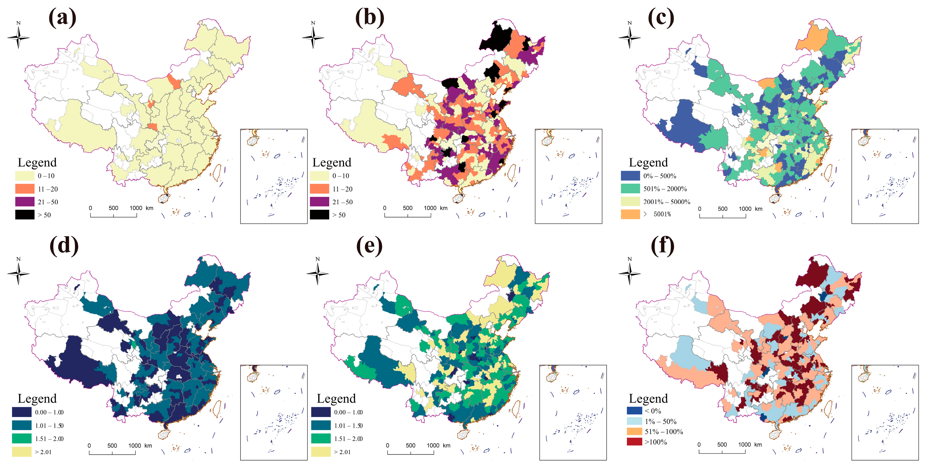
From a temporal perspective, GIAP development exhibited sustained expansion and steady growth between 2008 and 2024 (Figure 4a,b). In 2008, most cities had either not yet obtained GIAP certifications or had only a small number of certified products, with GIAP values concentrated primarily within the 0–10 range. Overall, GIAP development remained at a relatively early stage, with no pronounced spatial clustering. As the geographical indication protection system was progressively strengthened and supportive policies were expanded, the coverage of GIAP certification broadened steadily, accompanied by a continuous increase in development intensity. By 2024, GIAP values exceeded 10 in most cities, with moderate growth becoming increasingly widespread. This evolution suggests that GIAP development has gradually shifted from exploratory initiatives concentrated in a limited number of locations towards broader and more systematic expansion. Spatially, high-GIAP areas were primarily concentrated in northeastern China and the southeastern coastal regions, with spatial clustering becoming increasingly pronounced over time. GIAP development is relatively concentrated in northeastern, eastern and southeastern coastal regions, with expansion also observed in parts of central China. concentration and regional diffusion. Further examination of the spatial dynamics (Figure 4c) shows that GIAP values increased in the vast majority of cities, with particularly pronounced growth in eastern and central China. At the same time, GIAP growth remained relatively modest in some cities, suggesting persistent differences across regions in distinctive agricultural resource endowments, industrial foundations, and the institutional and market conditions underlying GIAP development.

By contrast, AGTFP exhibits substantially more complex and pronounced spatial heterogeneity. Overall, AGTFP increased steadily between 2008 and 2024, yet its spatial distribution displays a clear ‘low-coastal, high-inland’ pattern, with high-value areas concentrated predominantly in inland regions and relatively low values observed along the coast (Figure 4d,e). The spatial pattern of AGTFP growth further reveals a degree of regional differentiation, with the fastest-growing areas concentrated mainly in inland China, whereas coastal regions generally experienced comparatively slower growth (Figure 4f). Notably, this spatial configuration is partially misaligned with the distribution and growth of GIAPs. Regions with relatively high GIAP intensity and rapid GIAP expansion are concentrated primarily along the coast, whereas AGTFP exhibits a more pronounced inland advantage. This spatial divergence suggests that the development of GIAPs does not necessarily translate into contemporaneous improvements in agricultural green productivity at the same locations. Rather, the apparent spatial decoupling between GIAP development and AGTFP highlights the need to move beyond descriptive spatial patterns and further investigate the causal relationship, underlying mechanisms, and spatially differentiated effects linking GIAPs to agricultural green transformation.

4.2. Correlation Analysis

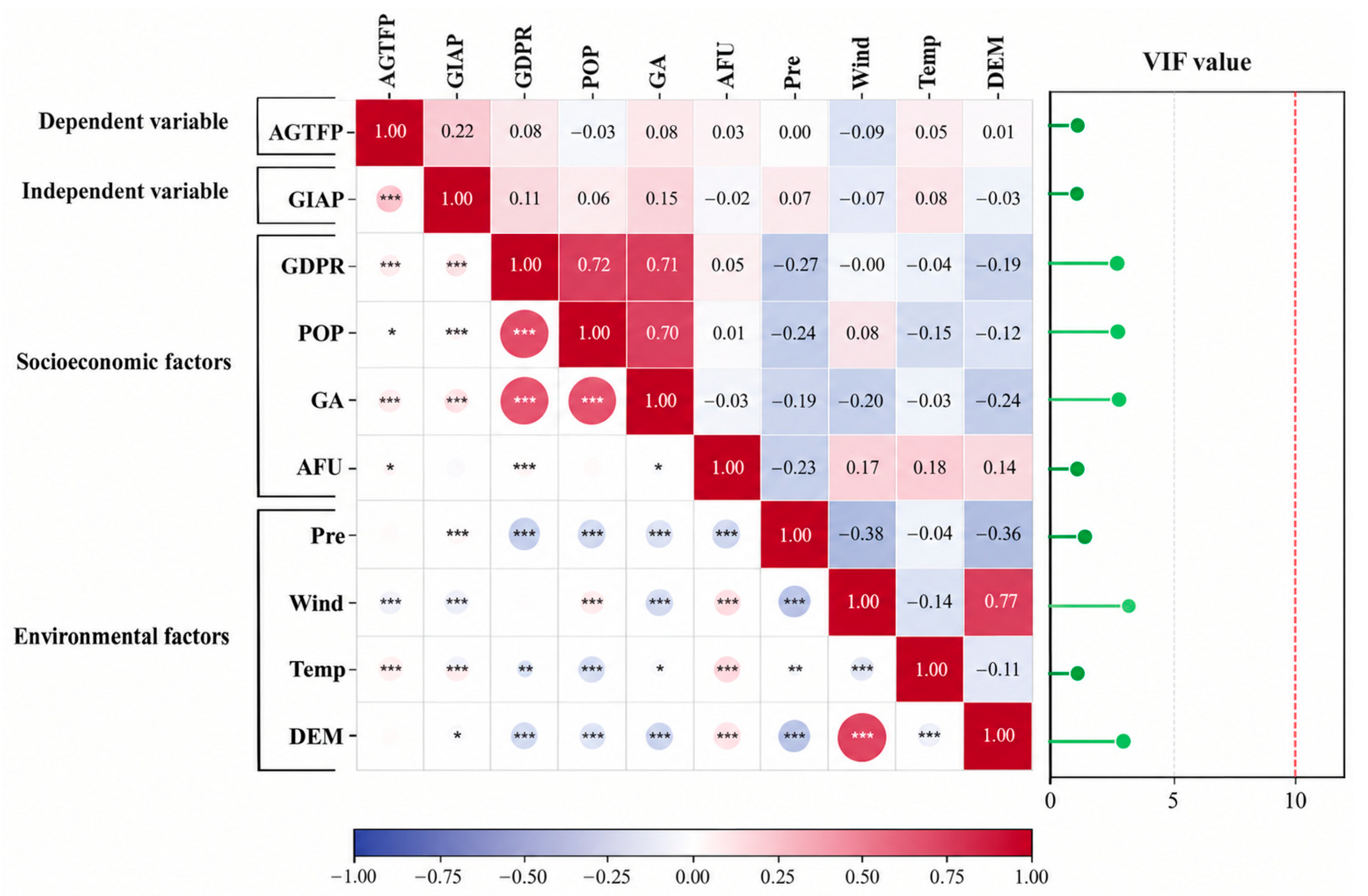
Prior to model estimation, we conducted correlation analysis and multicollinearity diagnostics. The results show that all variance inflation factor (VIF) values are below 10, indicating that none of the variables suffer from severe multicollinearity. The Pearson correlation matrix (Figure 5) further provides preliminary evidence for feature selection and hyperparameter optimization in the subsequent modeling framework.

The results reveal a significant positive correlation between GIAPs and AGTFP (r = 0.22, p ≤ 0.01), suggesting that cities with a greater number of GIAP certifications tend to exhibit higher levels of agricultural green productivity. Among the control variables, GDPR exhibits the strongest negative correlation with AGTFP (r = −0.08, p ≤ 0.01). In addition, wind speed (Wind) and population density (POP) are negatively associated with AGTFP (r = −0.09, p ≤ 0.01; r = −0.03, p ≤ 0.05). Although the correlation analysis provides preliminary evidence of a positive association between GIAPs and AGTFP, correlation alone cannot establish causal relationships or reveal the underlying mechanisms. Therefore, further analyses based on causal inference and interpretable machine learning approaches are required to identify the mechanisms through which GIAPs influence AGTFP and to uncover potential spatial heterogeneity.

4.3. DML Estimation

To identify the relationship between GIAPs and AGTFP, we employ a double machine learning (DML) framework based on Random Forests, incorporating city and year fixed effects to account for unobserved heterogeneity and potential confounding factors. To clarify the sample-splitting procedure, the initial 80/20 split was used for model development and tuning rather than for excluding observations from the final DML estimation. Specifically, the 80% subsample was used to develop the nuisance-function models, while the remaining 20% was used as an independent sample for model assessment. Within the model-development process, five-fold cross-fitting was conducted to obtain out-of-fold predictions of both the treatment and outcome nuisance functions. After the nuisance functions were specified, out-of-fold residuals were constructed for the observations used in the DML estimation, and the final orthogonalized treatment-effect coefficient was estimated using the full sample of 4930 observations. Therefore, the 20% subsample was not excluded from the final estimation sample reported in

Table 3. DML estimation results.

Variables	(1)	(2)	(3)	(4)
	AGTFP	AGTFP	AGTFP	AGTFP
GIAP	0.00172 *
	(1.77)
GIAP_A		0.00162 *
		(1.92)
GIAP_P			0.000744 ***
			(3.05)
GIAP_F				0.000689 **
				(2.43)
Std. Error	0.000971	0.000844	0.000244	0.000284
Control Variables	Yes	Yes	Yes	Yes
Machine Learning Model	Random Forest	Random Forest	Random Forest	Random Forest
Year FE	Yes	Yes	Yes	Yes
City FE	Yes	Yes	Yes	Yes
Obs	4930	4930	4930	4930

Note: Z statistics in parentheses. ***, **, and * refer to statistical significance at the 1%, 5%, and 10% levels, respectively. Standard error clustering at the city level.

. This procedure is distinct from the spatio-temporal holdout validation used to evaluate the predictive performance of OLS, GWR, RF, and GWRF.

The estimation results are reported in Table 3. The results indicate that GIAP development has a statistically significant positive effect on AGTFP, suggesting that the expansion of GIAP certification is associated with improvements in agricultural green total factor productivity. We further disaggregate GIAPs into three major product categories refer to product classification codes (GB/T 43583–2023): livestock-related GIAPs (GIAP_A), crop-based GIAPs (GIAP_P), and fishery-related GIAPs (GIAP_F). The results show that all three categories exert statistically significant positive effects on AGTFP, indicating that the green productivity-enhancing effect of GIAPs is not confined to a specific product category but extends across livestock, crop, and fishery products.

Statistical significance alone does not establish a causal relationship. Potential reverse causality between GIAPs and AGTFP, together with omitted-variable bias, may still give rise to endogeneity concerns. We therefore employ two complementary strategies to assess the causal interpretation of the baseline results. First, we adopt an instrumental variable. We construct an instrument by taking the interaction of the number of ancient academies (Unit: 100 academies) at the county level with a time trend and incorporate this instrument into the DML framework [52]. The validity of this instrument rests on two considerations. Regarding relevance, the development of GIAPs is closely associated with local historical and cultural characteristics, which are reflected in the historical presence of ancient academies [4]. Regarding the exclusion restriction, historical academies represent predetermined regional educational and cultural endowments established long before the modern GIAP certification system. Following prior studies using historical academies as instrumental variables [53], their locations are unlikely to have been systematically determined by contemporary agricultural or environmental conditions. Prefecture fixed effects absorb time-invariant regional characteristics, while year fixed effects capture common temporal shocks. Thus, we argue that the interaction is less likely to affect contemporary AGTFP through channels independent of GIAPs, although this exclusion restriction cannot be fully verified. The estimation results of the instrumental variables based on DML is presented in

Table 4. Endogeneity Issues.

Variables	(1)	(2)	(3)
	GIAP	AGTFP	AGTFP
Instrumental Variable	0.0508 **
	(2.16)
GIAP		0.00244 ***
		(2.82)
Treati × Posti,t			0.0592 **
			(2.58)
Std. Error	0.0235	0.00111	0.0235
Control Variables	Yes	Yes	Yes
Machine Learning Model	Random Forest	Random Forest	/
Time Fixed Effects	Yes	Yes	Yes
Individual Fixed Effects	Yes	Yes	Yes
Sample Size	4930	4930	4930
R2 Adjusted	/	/	0.548

Note: Z statistics in parentheses. *** and ** refer to statistical significance at the 1% and 5% levels, respectively. Standard error clustering at the city level.

column (1) and (2). In column (1), all instrumental variables exhibited significantly positive coefficients, providing evidence of instrument relevance. In column (2), the coefficient for GIAPs remained positive and was statistically significant at the 5% level, demonstrating that the findings from the baseline analysis are robust against potential endogeneity.

Second, we conduct an exogenous-shock using the four batches of National Lists of Advantageous Chinese Agricultural Products with Distinctive Characteristics released by the Ministry of Agriculture and Rural Affairs between 2017 and 2020 as an exogenous policy shock [54]. The baseline difference-in-differences model is specified as follows:

$$\begin{array}{c}{\mathit{AGTFP}}_{i,t}={\beta }_0+{\beta }_1{\mathit{Treat}}_i{\times \mathit{Post}}_{i,t}+{\beta }_n{X}_{i,t}+{\mu }_i{+\eta }_t+{ϵ}_{i,t}\end{array}$$

(8)

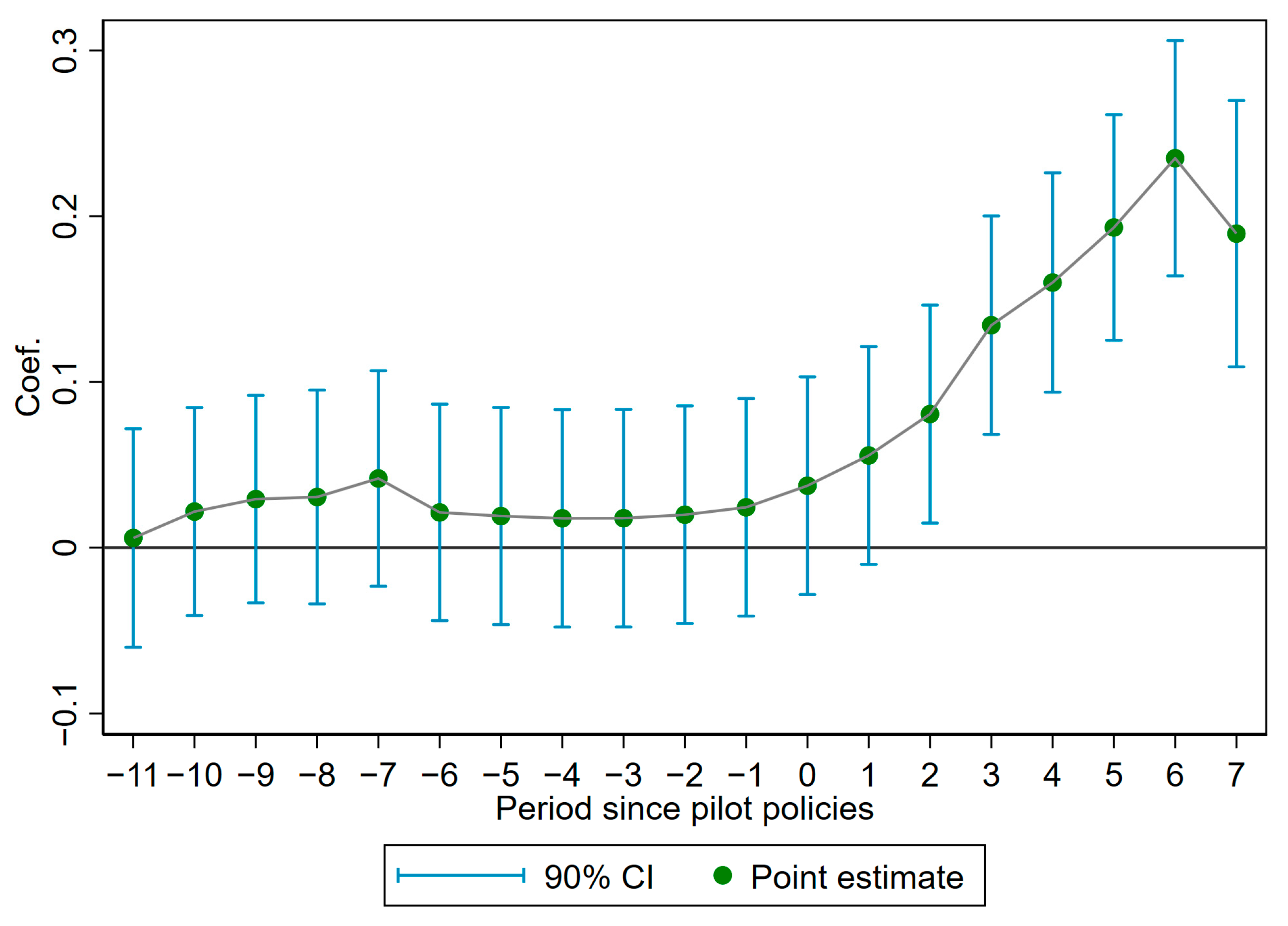
where Treat_i indicates whether city i belongs to the treatment group (1 = treated; 0 = control), and Post_i,t equals 1 in the first year that a treated city is included in the pilot program and 0 otherwise. $\sum X_{i,t}$ is a vector of control variables, μ_i and η_t capture city-specific and time-specific fixed effects, and ϵ_i,t is the error term. Table 4 column (3) indicates that the interaction term Treat×Post is significantly positive, suggesting that the pilot policy has a promoting effect on AGTFP. Furthermore, to examine the dynamic effects of this policy, we employed a parallel trends test model:

$$\begin{array}{c}{\mathit{AGTFP}}_{i,t}={\beta }_0+\sum {\beta }_m{\mathit{Treat}}_i{\times \mathit{Post}\left(n\right)}_{i,t}+{\beta }_n{X}_{i,t}+{\mu }_i{+\eta }_t+{ϵ}_{i,t}\end{array}$$

(9)

the estimated coefficients reflect the dynamic evolution of the relative treatment effect between the intervention group and the control group over eighteen periods (11 prior to policy implementation and 7 thereafter). The parallel trends test results are shown in Figure 6. Prior to the pilot policy implementation, no statistically significant impact on AGTFP was observed, further supporting the validity of the parallel trends assumption.

Further, we conduct a series of additional robustness checks to further assess the stability of the estimated effects. Detailed results for the robustness analyses are reported in the Supplementary Materials. Collectively, these analyses provide additional support for the robustness of the positive relationship between GIAPs and AGTFP.

4.4. Mechanism Identification

The theoretical framework suggests that GIAPs can enhance AGTFP through two key channels: agricultural industrial agglomeration (IA) and the downstream penetration of leading agricultural enterprises (AE). The results in columns (1) and (2) of

Table 5. Mechanism identification results.

Variables	(1)	(2)	(3)	(4)
	IA	AGTFP	AE	AGTFP
GIAP	0.00265 *		0.0000282 ***
	(1.74)		(3.11)
IA		0.0138 **
		(2.19)
AE				0.00952 ***
				(4.80)
Std. Error	0.00152	0.00630	0.00000907	0.00198
Control Variables	Yes	Yes	Yes	Yes
Machine Learning Model	Random Forest	Random Forest	Random Forest	Random Forest
Year FE	Yes	Yes	Yes	Yes
City FE	Yes	Yes	Yes	Yes
Obs	4930	4930	4930	4930

Note: Z statistics in parentheses. ***, **, and * refer to statistical significance at the 1%, 5%, and 10% levels, respectively. Standard error clustering at the city level.

show that GIAP development significantly promotes IA, while IA in turn has a significant positive effect on AGTFP. These findings are consistent with an indirect pathway through agricultural industrial agglomeration.

Columns (3) and (4) of Table 5 provide further evidence consistent with the second proposed mechanism. GIAP development is significantly associated with an increase in AE, while AE is positively associated with AGTFP. These results are consistent with an indirect pathway through leading agricultural enterprises. We further calculated the corresponding product-of-coefficients terms as a quantitative indication of the magnitude of these associations. The estimated products through IA and agricultural AE are approximately 0.000037 (=0.00265 × 0.0138) and 2.685 × 10⁻⁷ (=0.0000282 × 0.00952), respectively. Given that the outcome equations do not simultaneously control for GIAPs, however, these products should not be interpreted as conventional causal mediated effects; rather, they provide quantitative evidence consistent with the proposed transmission pathways. A plausible explanation is that GIAPs leverage regional brand value to attract production factors towards areas with distinctive agricultural advantages, thereby generating knowledge spillovers, technological diffusion, and resource-sharing effects that improve green production efficiency. At the same time, the stronger market incentives created by GIAPs encourage leading agricultural enterprises to enter producing regions and extend their operations towards the agricultural production frontier. These firms can transmit green technologies, production standards, and modern management practices to agricultural producers, thereby improving production organization and resource allocation. Through these complementary channels, GIAPs can facilitate the transition towards more efficient and environmentally sustainable agricultural production and ultimately enhance AGTFP.

4.5. Global Impact Analysis

To assess the relative importance of the multiple determinants of AGTFP, we conduct a global impact analysis using interpretable machine learning. After benchmarking the predictive performance of OLS, GWR, and RF models, we select geographically weighted random forest (GWRF) as the primary interpretability framework because of its superior ability to capture and explain spatially varying relationships. Detailed comparisons of model performance are reported in

Table 6. Model comparison.

Model	Dataset	R2	MSE	RMSE	MAE
GWR	Train	0.715	0.008	0.091	0.059
	Test	0.725	0.053	0.230	0.067
OLS	Train	0.128	0.084	0.298	0.235
	Test	0.436	0.160	0.399	0.383
Random Forest	Train	0.701	0.028	0.167	0.033
	Test	0.647	0.125	0.354	0.251
GWRF	Train	0.879	0.003	0.053	0.033
	Test	0.803	0.005	0.073	0.054

.

The RF and GWRF models were implemented in R using the randomForest and SpatialML packages, respectively. The global RF model was estimated with a fixed random seed of 12, 100 trees (ntree = 100), and a maximum tree depth of 20. The remaining hyperparameters followed the default settings of the randomForest package for regression, including mtry = max(floor(p/3), 1), sampling with replacement (replace = TRUE), and a minimum terminal-node size of 5 (nodesize = 5).

The GWRF model was implemented using the SpatialML package with a fixed random seed of 12. The local Random Forests followed the relevant default settings of SpatialML, including mtry = max(floor(p/3), 1) and impurity-based variable importance. Geographic weighting was enabled (geo.weighted = TRUE), and an adaptive bi-square kernel was employed. The bandwidth was defined by the number of geographically nearest neighboring cities rather than by a fixed geographic distance. Candidate neighborhood sizes were 40, 30, 20, 18, 16, 15, 12, and 10. Using the same spatial–temporal training sample described above, five-fold cross-validation was conducted for each candidate bandwidth. The bandwidth of 15 nearest neighboring cities yielded the lowest average RMSE and the highest average R² and was therefore selected as the final adaptive bandwidth. Here, “15 nearest neighbors” refers to 15 distinct geographically nearest cities, rather than 15 city-year observations. Detailed parameter settings and the bandwidth selection procedure are provided in the Supplementary Materials. Detailed comparisons of model performance are reported in Table 6.

We pool observations across all cities and years to construct the modeling dataset. Slightly different from the standard DML framework, we further accounted for both temporal and spatial heterogeneity when partitioning the data into training and testing sets. To prevent city-level spatial leakage, cities assigned to the testing set were completely excluded from the training sample across the entire study period. The training sample consists of observations from 2008 to 2018 for the remaining cities, whereas the testing sample consists exclusively of observations from 2019 to 2024 for the held-out cities. Within the training set, we employed a five-fold cross-validation strategy to evaluate model performance and improve the robustness of model specification. The training data were randomly divided into five mutually exclusive folds, with four folds used for model estimation and the remaining fold used for validation in each iteration. By jointly considering temporal extrapolation, spatial independence, and within-sample cross-validation, this design provides a rigorous evaluation framework that reduces the risk of overfitting and information leakage.

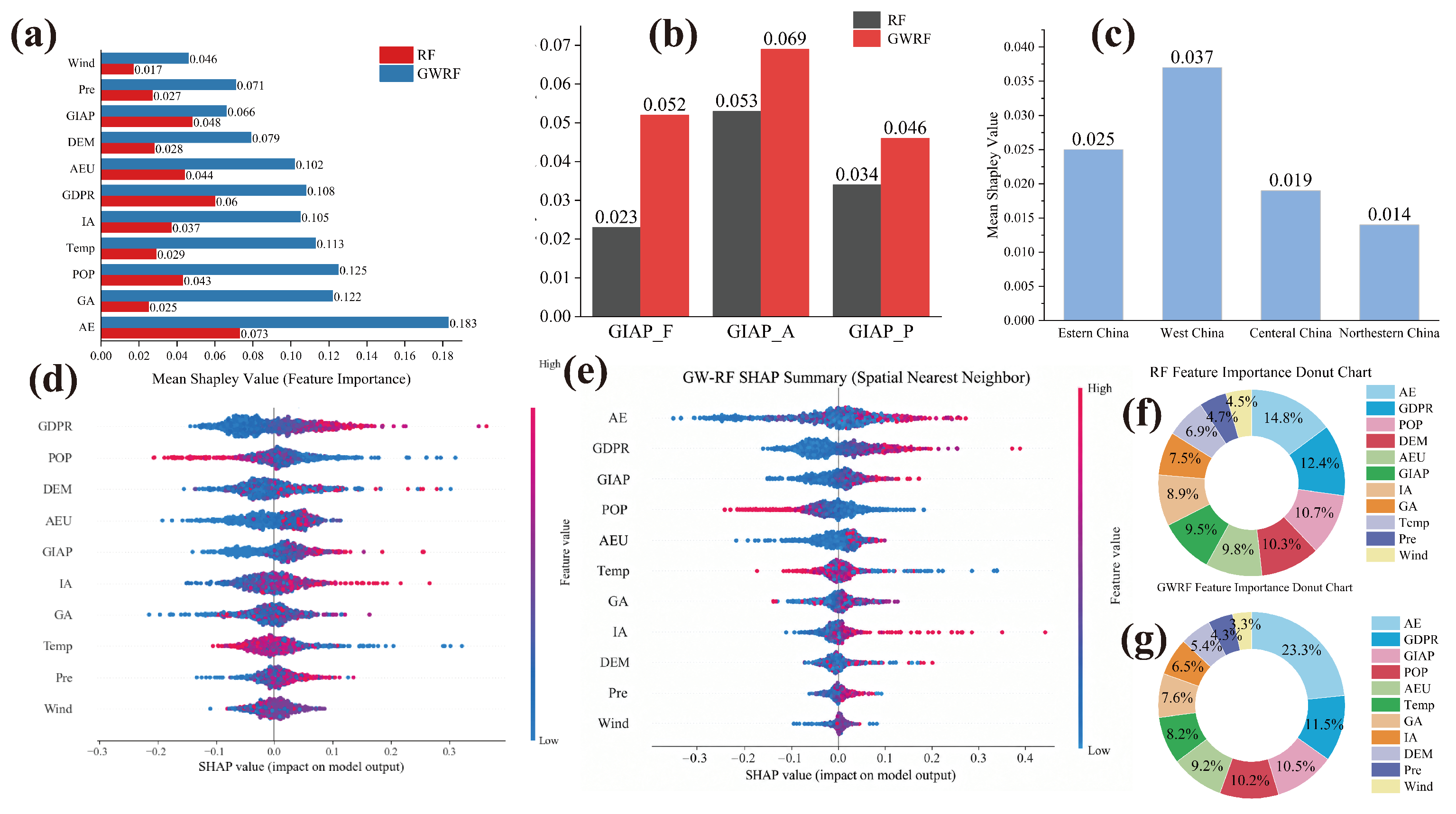
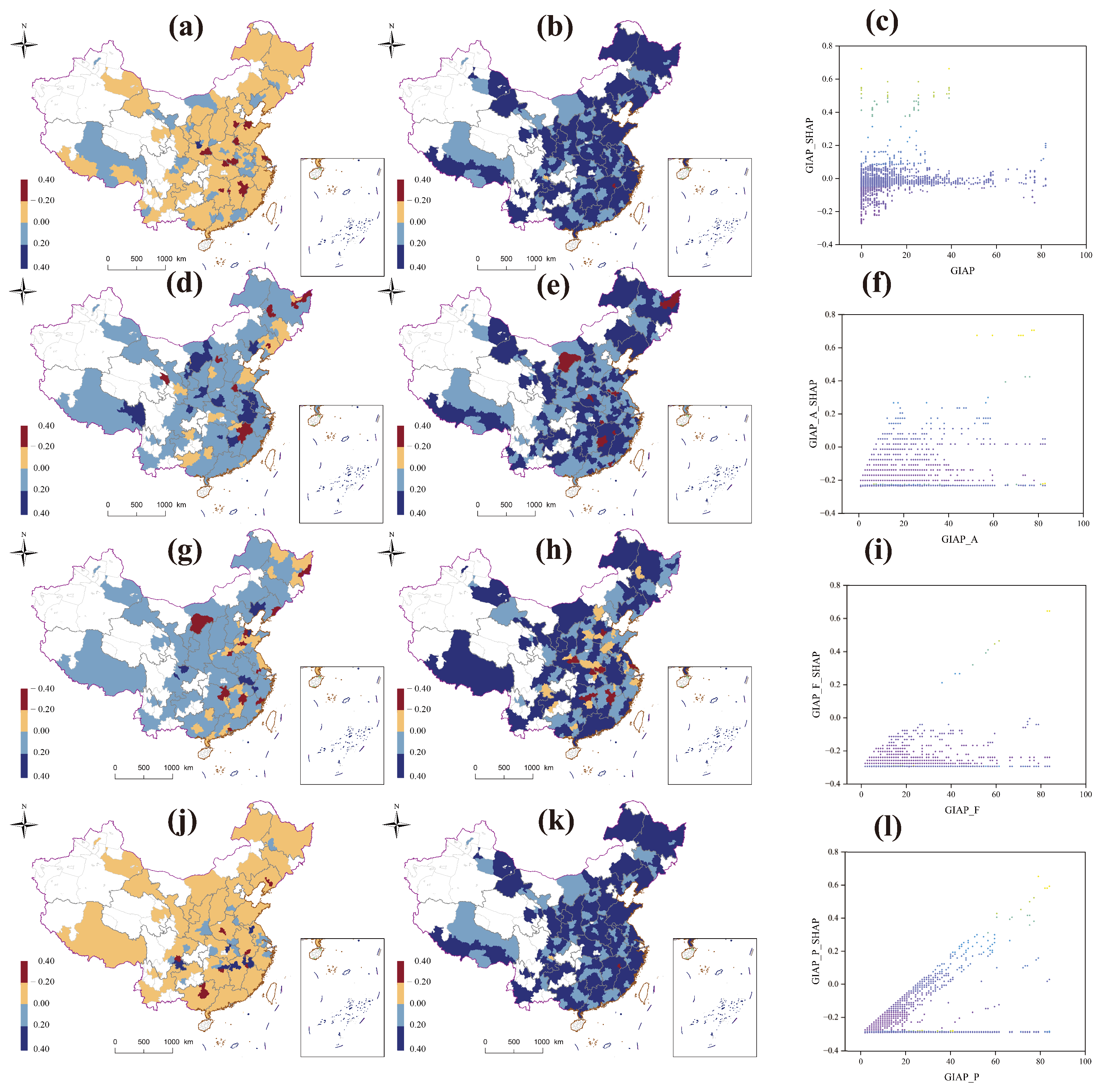
Feature importance is ranked according to the mean absolute SHAP values, and the results are compared between the conventional RF and GWRF models (Figure 7a). Three findings emerge. First, compared with the other predictors, GIAPs represent an important determinant of AGTFP within the predictive framework. Their mean absolute SHAP values are 0.066 and 0.048 across the corresponding analyses (Figure 7a), ranking fifth in the RF model (Figure 7d) and accounting for 9.5% of total feature importance (Figure 7f). In the GWRF model, GIAPs rise to third place (Figure 7e), with their contribution increasing to 10.5% of total feature importance (Figure 7g). This upward shift in ranking and relative contribution suggests that explicitly accounting for spatial heterogeneity provides additional information on the predictive importance of GIAPs for AGTFP.

Second, to examine heterogeneity across GIAP categories, we group and aggregate the SHAP results by product type (Figure 7b). The results reveal substantial differences in predictive importance across categories. Livestock-related GIAPs (GIAP_A) exhibit the strongest explanatory contribution, with a mean absolute SHAP value of 0.069 in the GWRF model. Fishery-related GIAPs (GIAP_F) rank intermediate, with a mean absolute SHAP value of 0.052, whereas crop-based GIAPs (GIAP_P) show the weakest contribution, with a mean absolute SHAP value of 0.046. These differences indicate that the predictive relevance of GIAPs for AGTFP varies systematically across product categories.

Third, we further examine regional heterogeneity by dividing the sample according to China’s major economic-geographical regions and comparing the mean absolute SHAP values from the RF model (Figure 7c). Western China exhibits the highest mean absolute SHAP value (0.037), followed by Eastern China (0.025), whereas Northeastern China records the lowest value (0.014). This regional variation indicates that the predictive contribution of GIAPs to AGTFP is strongly context dependent, with GIAP-related factors playing a more prominent role in explaining AGTFP variation in Western China than in the other regions.

4.6. Spatial Heterogeneity Analysis

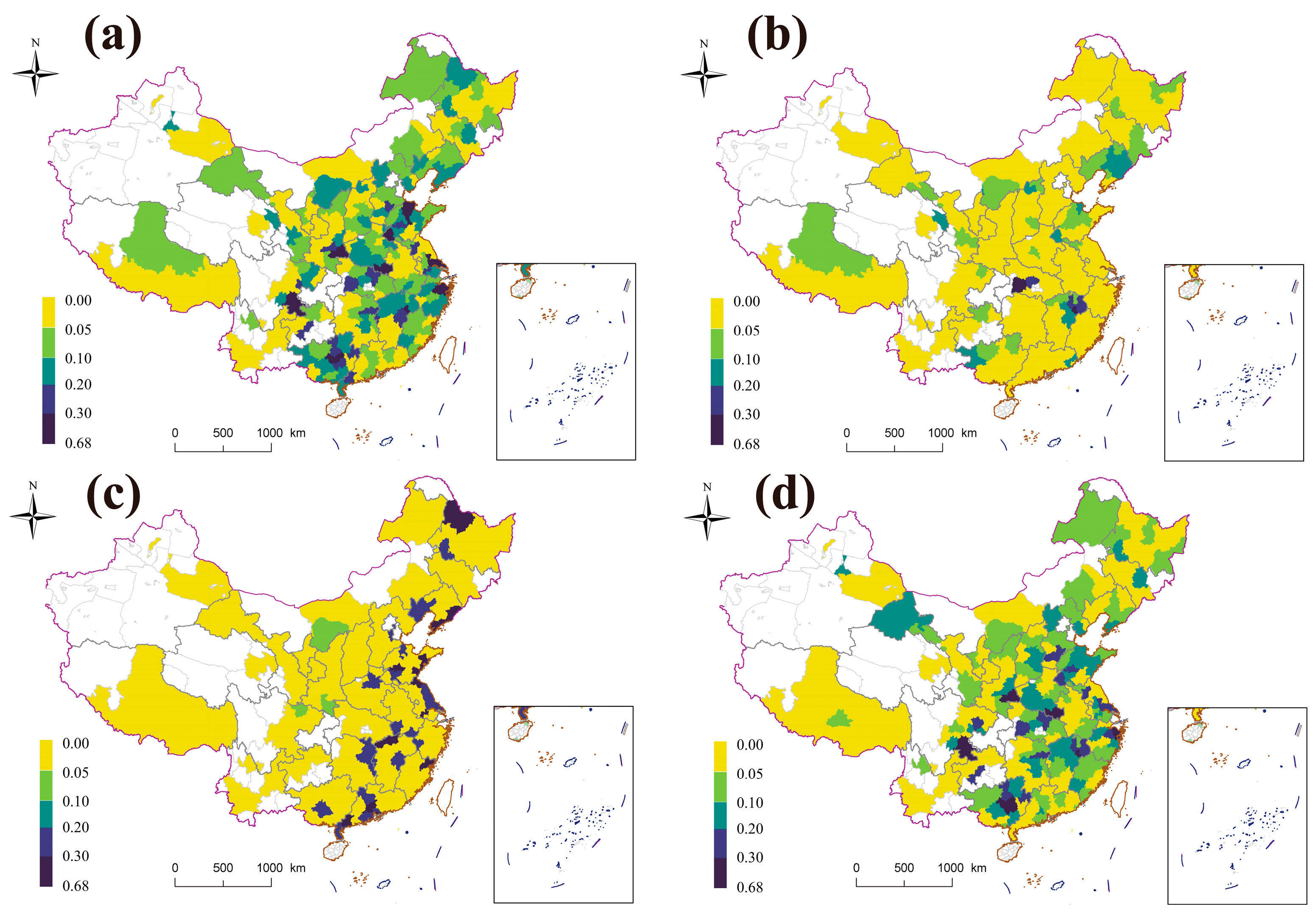
Because regional subgroup analyses cannot fully capture city-specific variation, we further investigate the spatial heterogeneity of GIAPs within the GWRF predictive framework. Specifically, we calculate local feature importance (FI) for each city based on the GWRF model. Local FI is defined as the average increase in prediction error resulting from randomly permuting a given feature while holding the remaining features unchanged. A higher FI therefore indicates a greater deterioration in local predictive performance after permutation, suggesting that the corresponding feature contains more information for explaining spatial variation in AGTFP at that location. Figure 8 presents the spatial distribution of the local FI of GIAPs and their major product categories.

The local FI of GIAPs and their product categories exhibits broadly consistent spatial patterns, characterized by a declining gradient from inland to coastal areas. Overall, GIAPs show relatively high local FI in inland regions but substantially lower FI in coastal cities (Figure 8a), indicating that GIAP-related information has greater local predictive relevance for AGTFP in inland areas. Notably, GIAP_A, GIAP_P, and GIAP_F exhibit broadly similar inland-to-coastal declining gradients in local FI (Figure 8b–d). This consistency suggests that the spatial differentiation in the predictive relevance of GIAPs is not specific to a particular product category. Rather, livestock, crop, and fishery-related GIAPs display broadly convergent spatial patterns in their predictive relevance to AGTFP, although their local magnitudes and spatial distributions differ to some extent. Taken together, these findings reveal substantial spatial heterogeneity in the predictive relevance of GIAPs for AGTFP.

Figure 9 presents the spatial distribution and dependence plots of SHAP values for GIAPs and their major product categories. The spatial distributions are compared between 2008 and 2024 to examine how the predictive contributions of GIAPs have evolved over time. Overall, the SHAP values of GIAP, GIAP_A, GIAP_P, and GIAP_F generally increase over the study period, while their spatial distributions exhibit a broadly consistent inland-high and coastal-low gradient. For GIAPs as a whole, SHAP values are relatively high and predominantly positive in inland regions, indicating that the observed GIAP characteristics in these cities contribute positively to the GWRF prediction of AGTFP relative to the model baseline. Coastal cities also generally exhibit positive SHAP values, but their magnitudes are smaller than those observed inland, suggesting that GIAP-related information makes a weaker positive contribution to local AGTFP predictions in coastal areas (Figure 9a,b). A broadly similar spatial pattern is observed for crop-based GIAPs (GIAP_P), whose SHAP values are predominantly positive and relatively high in inland regions but lower along the coast (Figure 9j,k).

However, the spatial patterns of different GIAP categories are not completely uniform. For livestock-related GIAPs (GIAP_A), negative SHAP values emerge in some parts of northeastern China (Figure 9d,e). This indicates that, within the local GWRF predictions and conditional on the other features included in the model, the observed GIAP_A characteristics in these locations are associated with predictions of AGTFP below the corresponding model baseline. Similarly, fishery-related GIAPs (GIAP_F) exhibit negative SHAP values in parts of central China (Figure 9g,h), suggesting that the observed GIAP_F characteristics in these locations make a negative contribution to the model’s local AGTFP prediction relative to the baseline.

5. Discussion

5.1. Environmental Foundations and Social Economic Development Jointly Shape the Spatial Divergence Between GIAPs and AGTFP

The spatial divergence between GIAP development and AGTFP is not driven by a single factor but instead reflects the combined influence of ecological foundations, economic development, and regional agricultural transformation trajectories. Our findings reveal that high-GIAP regions are primarily concentrated in northeastern and southeastern coastal China, where geographical indication development has gradually formed stable spatial clusters. In contrast, regions with higher AGTFP levels and faster growth are more frequently observed in inland areas, resulting in a notable spatial mismatch between GIAP development and agricultural green productivity. This divergence may partly reflect differences in the marginal returns to development. In coastal regions, the long-term intensification of agricultural inputs and production activities may have generated diminishing marginal gains in green productivity, while dense economic and agricultural agglomeration may also place greater pressure on local ecological carrying capacity. By contrast, inland regions may benefit from a catch-up process associated with technological diffusion, improved infrastructure, and the adoption of more advanced green production practices from developed regions. Such technological convergence can enable inland areas to improve resource-use efficiency and reduce environmental pressures without requiring a comparable level of GIAP concentration.

Environmental conditions and resource endowments provide the basic foundation for GIAP development. As a place-based agricultural intellectual property system, GIAPs are closely related to local climate, soil, water resources, and traditional production practices. Regions with rich ecological resources and well-developed agricultural systems are more likely to produce agricultural products with clear geographical characteristics and strong market recognition. At the same time, economic development and market access can further increase the concentration of GIAPs. Coastal regions usually have better transportation networks, market systems, industrial infrastructure, and commercialization capacity. These conditions make it easier to obtain GIAP certification, build brands, and increase product value. As a result, these regions are more likely to have higher GIAP accumulation and stronger spatial clustering.

However, AGTFP reflects the balance between agricultural economic output, resource inputs, and environmental constraints, rather than simply the level of agricultural commercialization or market development. Coastal regions have stronger economies and more developed agricultural markets, but they also face greater pressures from limited land, high factor inputs, and environmental problems. In contrast, many inland regions have more agricultural resources and ecological space. They also have more room to improve production efficiency and adopt greener production technologies. These differences may lead to higher AGTFP levels and greater growth potential in inland areas.

The spatial mismatch between GIAPs and AGTFP suggests that agricultural branding and green productivity improvement are not inherently equivalent processes. GIAP development primarily reflects the market-oriented realization of regional agricultural advantages, whereas AGTFP depends on the coordinated optimization of economic returns, resource utilization, technological progress, and ecological constraints. Therefore, promoting green agricultural transformation through GIAPs should not rely solely on expanding certification scale. Instead, policy efforts should focus on strengthening the integration of GIAP development with green technologies, efficient resource allocation, and ecological value realization, while tailoring development strategies to regional resource conditions and agricultural transformation stages.

5.2. Spatial Heterogeneity in the Predictive Contribution of GIAPs to AGTFP

The FI and SHAP analyses jointly reveal substantial spatial heterogeneity in the predictive relevance of GIAPs for AGTFP. The spatial distribution of FI indicates that the local importance of GIAPs and their product categories generally follows a declining gradient from inland to coastal regions, suggesting that GIAP-related characteristics contain more information for explaining AGTFP variation in inland areas. The SHAP analysis further demonstrates that this spatial heterogeneity extends beyond feature importance to the direction and magnitude of GIAP-related contributions to AGTFP predictions. During 2008–2024, the SHAP values of GIAPs and their different categories generally increased, with inland regions consistently exhibiting stronger positive SHAP contributions than coastal regions. This pattern shows that GIAP-related information has become more useful for explaining differences in AGTFP over time. It also shows clear spatial differences.

This spatial difference may be related to differences in GIAP development stages, agricultural industrial structures, and regional transformation capacity. In coastal regions, GIAP development started earlier and has been supported by more developed industrial systems, market systems, and branding strategies. As a result, one possible explanation is that GIAP-related features may already be closely linked to local agricultural production systems, market networks, and industrial organizations. In the GWRF model, GIAPs may therefore provide less new information for explaining differences in AGTFP among coastal cities, leading to lower FI and SHAP values. In contrast, inland regions often have more distinctive agricultural resources and closer links between GIAP development and local agricultural transformation. Therefore, GIAP-related features may better reflect differences in agricultural production and green transformation potential, leading to higher local feature importance and stronger positive SHAP values.

The comparison of GIAP categories shows both common spatial patterns and category-specific differences. Crop-based GIAPs (GIAP_P) show a spatial pattern of SHAP values that is similar to the overall GIAP pattern, with stronger contributions in inland regions and weaker contributions in coastal areas. This suggests that the predictive role of crop-based GIAPs is relatively stable across regions. However, livestock-related GIAPs (GIAP_A) and fishery-related GIAPs (GIAP_F) show negative SHAP values in some areas. In particular, negative SHAP contributions appear for GIAP_A in parts of northeastern China and for GIAP_F in some central regions. These results mean that, after considering the other features in the model, the observed values of these GIAP categories are linked to lower predicted AGTFP than the model’s baseline prediction in these areas.

5.3. Differentiated Agricultural Green Transformation Strategies

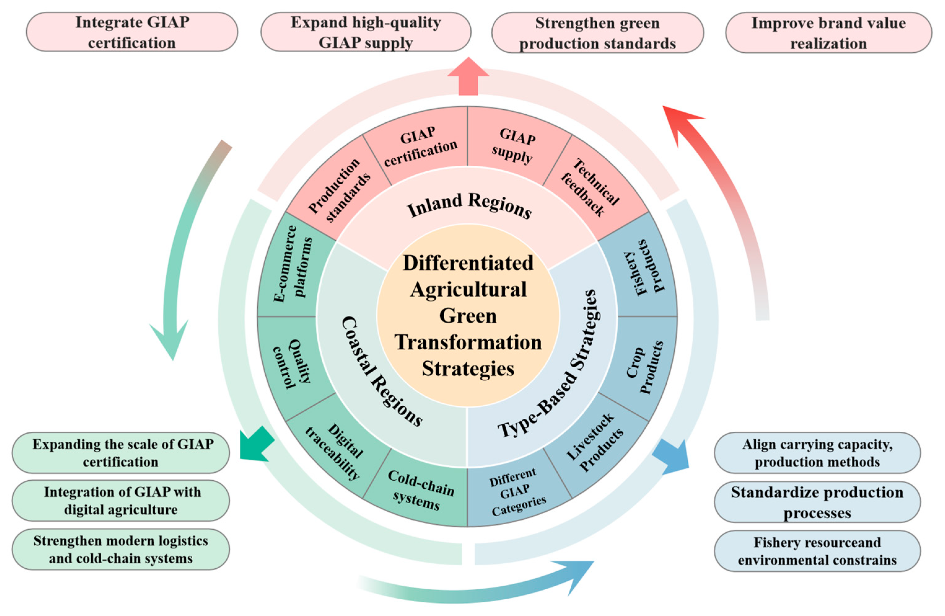
The above findings demonstrate that the predictive relevance of GIAPs for AGTFP varies substantially across regions and product categories. Therefore, agricultural green transformation should not rely on a one-size-fits-all approach but instead adopt differentiated strategies that account for regional resource endowments, industrial foundations, and GIAP characteristics. The differentiated agricultural green transition strategy is shown in Figure 10.

For coastal regions, the relatively lower FI and SHAP values of GIAPs do not imply limited development potential. Instead, they suggest that GIAP-related information may overlap more strongly with other advanced agricultural development factors, such as mature market systems, industrial integration, and technological capabilities. Therefore, coastal regions should shift from pursuing quantitative expansion of GIAP certification towards improving certification quality and strengthening industrial integration. Greater emphasis should be placed on integrating GIAPs with digital agriculture, green technological innovation, modern logistics systems, and advanced agricultural processing to enhance their contribution to agricultural green transformation. In practice, local governments can establish quality-oriented certification and dynamic monitoring mechanisms, while encouraging GIAP enterprises and cooperatives to integrate digital traceability, quality control, cold-chain logistics, and e-commerce platforms into the entire value chain. This would facilitate the transformation of GIAPs from a certification label into an integrated brand asset embedded in production, marketing, logistics, and consumer services.

For inland regions, policy attention should focus on converting their potential for green productivity improvement into standardized and scalable production practices. Given the relatively fragmented structure of small-scale farming, local governments can strengthen linkages between GIAP organizations and leading agricultural enterprises, cooperatives, and agricultural service providers. Leading enterprises can establish unified production standards covering input use, pesticide and fertilizer application, resource conservation, and waste management, while providing farmers with technical training, input guidance, quality inspection, and purchase contracts. Digital platforms can further support production-record management and traceability, enabling enterprises to monitor compliance and provide targeted technical feedback. Such institutional arrangements can reduce coordination costs among dispersed farmers and promote the diffusion of eco-friendly practices across fragmented agricultural production systems.

Differences across GIAP categories show the need for targeted development strategies. For livestock-related GIAPs, negative SHAP contributions in some northeastern regions suggest that increasing certification alone may not improve green productivity. Development strategies should pay more attention to the fit between regional resource capacity, production systems, and industrial structures. Improving green production standards, using resource-saving technologies, and improving livestock value chains can help make livestock GIAP development more consistent with AGTFP improvement.

For crop-based GIAPs, the broadly consistent spatial pattern of SHAP contributions across regions suggests a relatively stable predictive contribution to agricultural green transformation. Future efforts should focus on brand development, industrial agglomeration, and standardized production systems. These measures can help turn existing advantages into lasting improvements in agricultural green productivity. For fishery-related GIAPs, negative SHAP values in some central regions suggest that the benefits of certification depend on its compatibility with local ecological carrying capacity. Simply expanding certifications without considering water resources, production intensity, and aquatic ecosystem conditions may be associated with more intensive aquaculture activities, increasing nutrient loads and pollution-treatment pressure and thereby generating negative environmental externalities and efficiency losses. Local authorities should therefore avoid treating certification expansion as an independent policy target. Instead, GIAP development should be aligned with local water-environment capacity through ecological aquaculture, optimized fishery structures, and resource-efficient production. Certification approval and subsequent monitoring can also incorporate ecological capacity assessments, water-quality monitoring, and production traceability to ensure that GIAP expansion remains compatible with ecosystem resilience and contributes to sustainable agricultural green productivity.

Overall, the effect of GIAPs on agricultural green transformation depends not only on certification but also on how GIAP development fits local ecological conditions, industrial systems, and technological capacity. Therefore, different GIAP types should be developed according to local conditions to better improve agricultural green productivity.

5.4. Limitations

This study examines the impact of GIAPs on AGTFP using a balanced panel dataset of 290 Chinese cities from 2008 to 2024. By combining causal inference and interpretable machine learning methods, we examine the overall effects, possible mechanisms, and spatial differences in GIAPs in agricultural green transformation. However, this study still has several limitations.

First, this study uses prefecture-level cities as the main research units because of data availability. Although the city-level analysis captures regional differences in GIAP development and agricultural green productivity, the relatively large spatial units may hide smaller-scale differences and local mechanisms. Future research could use county-level or village-level data. More detailed data could help identify the local effects and spatial boundaries of GIAPs on agricultural transformation.

Second, this study mainly examines the relationship between GIAPs and AGTFP from a regional perspective. It focuses on agricultural industrial agglomeration and the role of leading agricultural enterprises as the main channels. However, GIAPs may also affect AGTFP through changes in farmers’ production decisions, firms’ technology adoption, and participation in agricultural cooperatives or producer organizations. Future studies could combine household survey data, firm-level data, and organizational data to better understand the micro-level mechanisms behind the relationship between GIAPs and agricultural green transformation.

Third, this study also has limitations regarding variable construction. First, concerning the input side of AGTFP, due to data constraints, we estimated the municipal irrigation area by multiplying the provincial effective irrigation ratio by the number of municipal administrative areas. Although we have referenced relevant literature, cities within the same province share key components of this structural indicator, which may introduce bias in the estimation of AGTFP’s input in this component.

Fourth, this study combines double machine learning (DML) and GWRF-SHAP to examine the effects and spatial differences in GIAPs. DML can reduce estimation bias caused by high-dimensional covariates and flexible functional forms. However, causal interpretation still depends on identification assumptions, and some endogeneity problems may remain. Furthermore, the selection of the instrumental variable also has limitations. Based on the time-invariant and time-varying principles, we construct the instrument by interacting historical academies with a time trend. Although prefecture fixed effects absorb time-invariant regional differences, this interaction may still capture heterogeneous development trajectories that are correlated with contemporary agricultural productivity. Therefore, the exclusion restriction may not be fully guaranteed, and the instrumental variable estimates should be interpreted with appropriate caution. In addition, machine learning models can also capture nonlinear relationships and interactions between variables. Therefore, this study further uses partial dependence plots to examine the nonlinear relationship between GIAPs and AGTFP. The additional results are provided in the Supplementary Materials.

Finally, GWRF provides useful information on spatial differences, but the relationship between GIAPs and AGTFP may also change over time. Future research could combine spatiotemporal models with machine learning methods to examine both spatial and temporal differences. This approach could provide a better understanding of how GIAPs affect agricultural green productivity as economic, technological, and environmental conditions change.

6. Conclusions

Using a balanced panel dataset of 290 Chinese cities from 2008 to 2024, this study examines the role of geographical indication agricultural products (GIAPs) in improving agricultural green total factor productivity (AGTFP). By combining causal inference and interpretable machine learning methods, we examine the changes in GIAPs and AGTFP over time and across regions, identify the main mechanisms, and examine differences across regions and GIAP types. The main findings are as follows.

First, both GIAPs and AGTFP increased during the study period, but their spatial patterns were different. High-GIAP regions were mainly located in northeastern and southeastern coastal China, where GIAPs gradually formed clear spatial clusters. In contrast, high-AGTFP regions were mainly found in inland areas, showing a clear “low-coastal, high-inland” pattern. This difference shows that the growth of GIAPs and AGTFP does not always occur in the same areas.

Second, the DML results show that GIAPs significantly improve AGTFP. This positive effect remains after addressing possible endogeneity and conducting several robustness checks. Mechanism analysis shows that GIAPs improve AGTFP mainly through agricultural industrial agglomeration (IA) and the downstream penetration of leading agricultural enterprises (AE). On the one hand, the brand value of GIAPs attracts production factors to regions with distinctive agricultural products. This can promote knowledge sharing, technology diffusion, and green production efficiency. On the other hand, GIAPs can encourage leading agricultural enterprises to enter producing regions. These firms can help spread green technologies, production standards, and modern management practices across agricultural value chains.

Third, the GWRF-SHAP results show clear spatial and product-type differences in the predictive role of GIAPs for AGTFP. Overall, GIAPs and their main categories have higher feature importance and stronger positive predictive contributions in inland regions than in coastal areas. However, some GIAP categories show negative SHAP contributions in certain areas. This suggests that the relationship between GIAPs and AGTFP depends on regional resources, industrial conditions, and product characteristics. Therefore, GIAP development should follow different strategies based on local conditions, industrial structures, and ecological constraints.

References

1. Song, Q.; Liu, Q. Does Environmental Enforcement Promote Agricultural Green Productivity? The Moderating Roles of Land Transfer and Insurance. Agriculture 2026, 16, 1360. [Google Scholar] [CrossRef] [Scilit]
2. Wei, W.; Cui, Q.; Sheng, Y. Dual Carbon Goals and the Impact on Future Agricultural Development in China: A General Equilibrium Analysis. China Agric. Econ. Rev. 2022, 14, 664–685. [Google Scholar] [CrossRef] [Scilit]
3. Guo, H.; Wang, X.; Xia, H.; Jiang, W. Digital Villages and Agricultural Green Total Factor Productivity: A Supply-Side and Demand-Side Mechanism Analysis. Front. Sustain. Food Syst. 2026, 10, 1831978. [Google Scholar] [CrossRef] [Scilit]
4. Liao, K.; Li, C.; Jiang, L. How Geographical Indication Products Impact Agricultural Economic Resilience: Evidence from China. China Econ. Rev. 2025, 94, 102527. [Google Scholar] [CrossRef] [Scilit]
5. Ming, Z.; Yang, B. The Impact of Geographical Indications of Agricultural Products on Agricultural Industry Resilience at the County Level. Res. Agric. Mod. 2025, 46, 930–941. [Google Scholar] [CrossRef]
6. Curzi, D.; Huysmans, M. The Impact of Protecting EU Geographical Indications in Trade Agreements. Am. J. Agric. Econ. 2022, 104, 364–384. [Google Scholar] [CrossRef] [Scilit]
7. Deng, S.; Wei, Q.; Hong, Y.; Liu, H. Digital Highways and Green Agricultural Productivities: Evidence from County-Level Panel Data in China. J. Clean. Prod. 2026, 562, 148450. [Google Scholar] [CrossRef] [Scilit]
8. Gong, B. Agricultural Productivity Convergence in China. China Econ. Rev. 2020, 60, 101423. [Google Scholar] [CrossRef] [Scilit]
9. Chen, S.; Gong, B. Response and Adaptation of Agriculture to Climate Change: Evidence from China. J. Dev. Econ. 2021, 148, 102557. [Google Scholar] [CrossRef] [Scilit]
10. Lee, C.-C.; Lee, C.-C. How Does Green Finance Affect Green Total Factor Productivity? Evidence from China. Energy Econ. 2022, 107, 105863. [Google Scholar] [CrossRef] [Scilit]
11. Sun, Y. Environmental Regulation, Agricultural Green Technology Innovation, and Agricultural Green Total Factor Productivity. Front. Environ. Sci. 2022, 10, 955954. [Google Scholar] [CrossRef] [Scilit]
12. Jiang, J.; Wang, Z.; Wang, Y.; Yang, Q.; Chu, Y.; Wang, S. Spatio-Temporal Differentiation Patterns and Income Increasing Mechanisms of Geographical Indication Agricultural Products in China. Acta Geogr. Sin. 2026, 81, 1549–1567. [Google Scholar] [CrossRef]
13. Zhao, T.; Yu, X.; Liu, S. Research on the Co-Creation Mechanism of Geographical Indication Industry Value Based on Evolutionary Game Analysis. Sustainability 2024, 16, 2075. [Google Scholar] [CrossRef] [Scilit]
14. Lu, F.; Zhang, G.; Wang, T.; Ye, Y.; Zhao, Q. Geographically Weighted Random Forest Based on Spatial Factor Optimization for the Assessment of Landslide Susceptibility. Remote Sens. 2025, 17, 1608. [Google Scholar] [CrossRef] [Scilit]
15. Qin, S.; Han, Z.; Chen, H.; Wang, H.; Guo, C. High-Quality Development of Chinese Agriculture under Factor Misallocation. Int. J. Environ. Res. Public Health 2022, 19, 9804. [Google Scholar] [CrossRef] [Scilit]
16. Zhang, Y.; Liu, Y. Geographical Indication Certification of Agricultural Products and Agricultural Carbon Emissions—Empirical Evidence from China. Front. Sustain. Food Syst. 2025, 9, 1644196. [Google Scholar] [CrossRef] [Scilit]
17. Xiao, R.; Zhao, P.; Qi, Y.; Lu, Y. The Spatial Heterogeneity Characteristics and the Influencing Factors of the Agro-Product Geographical Indication Brands. Res. Agric. Mod. 2021, 42, 1126–1136. [Google Scholar] [CrossRef]
18. Xu, X.; Sheng, Y.; Ball, E. Is There a ‘Price’to Pay for Agricultural TFP Measurement? Limitations of the Distance Function Approach. Aust. J. Agric. Resour. Econ. 2025, 69, 662–673. [Google Scholar] [CrossRef] [Scilit]
19. Zou, C.; Zou, Z. Can Certification of Geographical Indication Agricultural Products Promote Agricultural Green Total Factor Productivity? Evidence on Moderation and Threshold Effects from China. Sustainability 2026, 18, 8265. [Google Scholar] [CrossRef] [Scilit]
20. Huang, X.; Feng, C.; Qin, J.; Wang, X.; Zhang, T. Measuring China’s Agricultural Green Total Factor Productivity and Its Drivers during 1998–2019. Sci. Total Environ. 2022, 829, 154477. [Google Scholar] [CrossRef] [Scilit]
21. Yang, Y.; Lian, D.; Zhang, Y.; Wang, D.; Wang, J. Analysis of the Impact of Resource Misallocation and Socialized Services on Low-Carbon Agricultural Production with DML Based on Random Forest. Int. Rev. Econ. Finance 2024, 95, 103452. [Google Scholar] [CrossRef] [Scilit]
22. Qin, Z.; Peng, Q.; Jin, C.; Xu, J.; Xing, S.; Zhu, P.; Yang, G. Geographically Weighted Random Forest Fusing Multi-Source Environmental Covariates for Spatial Prediction of Soil Heavy Metals. Environ. Pollut. 2025, 385, 127135. [Google Scholar] [CrossRef] [Scilit]
23. Song, Y.; Zhu, W.; Yang, Y.; Su, E. Agriculture-Service Integration and Agricultural Green Total Factor Productivity: A Case Study of China. Socioecon. Plan. Sci. 2025, 102, 102326. [Google Scholar] [CrossRef] [Scilit]
24. Ren, J.; Wang, M.; Li, X.; Ding, X. Data Elements and Agricultural Green Total Factor Productivity: Evidence from a Quasi-Natural Experiment Based on Public Data Openness in China. Agriculture 2025, 15, 1130. [Google Scholar] [CrossRef] [Scilit]
25. Mao, H.; Zhou, L.; Ying, R.; Pan, D. Time Preferences and Green Agricultural Technology Adoption: Field Evidence from Rice Farmers in China. Land Use Policy 2021, 109, 105627. [Google Scholar] [CrossRef] [Scilit]
26. Wei, Z.; Peng, J.; Zhao, Y.; Li, X.; Wang, C. Reform of Agricultural Land Property Rights System and Grain Production Resilience: Empirical Evidence Based on China’s “Three Rights Separation” Reform. PLoS ONE 2025, 20, e0319387. [Google Scholar] [CrossRef] [Scilit]
27. Dang, G.; Guo, Y.; Zhang, L. Mechanisms and Paths of Geographical Indications Promoting the Construction of a Beautiful and Harmonious Countryside in Ethnic Mountainous Areas: An Analysis from the Perspective of New Endogenous Development. Chin. Rural Econ. 2024, 7, 96–118. [Google Scholar] [CrossRef]
28. Fernández-Zarza, M.; Amaya-Corchuelo, S.; Belletti, G.; Aguilar-Criado, E. Trust and Food Quality in the Valorisation of Geographical Indication Initiatives. Sustainability 2021, 13, 3168. [Google Scholar] [CrossRef] [Scilit]
29. Zhang, Y.; Huang, Y. Research on the Influence of Geographical Indication Brand Participation on the Quality and Safety of Agricultural Products. J. Huazhong Agric. Univ. Sci. Ed. 2022, 3, 123–135. [Google Scholar] [CrossRef]
30. Lou, B.; Fu, X.; Xue, B. Effectiveness, Problems, and Transformation of Geographical Indications in the Context of Rural Revitalization: Evidence from Pengshui in Chongqing. Sustainability 2023, 15, 8870. [Google Scholar] [CrossRef] [Scilit]
31. Yang, F.; Gan, W.; Song, Z. The Economic and Ecological Effects of Agricultural Geographical Indication Certification in Hilly and Mountainous Areas: Mechanism Analysis and Empirical Evidence. Geogr. Res. 2026, 2, 532–546. [Google Scholar]
32. Ellison, G.; Glaeser, E.L.; Kerr, W.R. What Causes Industry Agglomeration? Evidence from Coagglomeration Patterns. Am. Econ. Rev. 2010, 100, 1195–1213. [Google Scholar] [CrossRef] [Scilit]
33. Chen, B.; Yang, F. The County-Level Economic Growth Effect of Characteristic Agricultural Development Policy Implementation: An Assessment Based on Chinese Characteristic Agricultural Product Advantage Zones. Rural Econ. China 2024, 10, 132–152. [Google Scholar] [CrossRef]
34. Zeng, L.; Li, Z. Research on the Impact of Rural Collective Property Rights System Reform on Rural Industrial Integration-the Yangtze River Economic Belt as an Example. Front. Sustain. Food Syst. 2025, 9, 1593519. [Google Scholar] [CrossRef] [Scilit]
35. Yin, X.Y.; Jia, X.J.; Li, D.M. The Empact of Agricultural Industrial Agglomeration on Green Total Factor Productivity—Based on the Perspective of Spatial Spillover Effect. Chin. J. Agric. Resour. Reg. Plan. 2022, 43, 110–119. [Google Scholar] [CrossRef]
36. Xu, X.; Wu, B. Are Cooperatives an Ideal Carrier for the Organic Connection between the Production of Small Farmers and the Development of Modern Agriculture? Rural Econ. China 2018, 11, 80–95. [Google Scholar] [CrossRef]
37. Jin, Q.; Dang, H.; Wang, H.; Zhang, Z. Exploring Cooperative Mechanisms in the Chinese Agricultural Value Chain: A Game Model Analysis Based on Leading Enterprises and Small Farmers. Agriculture 2024, 14, 437. [Google Scholar] [CrossRef] [Scilit]
38. Wang, T.; Ma, Y.; Luo, S. Spatial Pattern and Influencing Factors of Agricultural Leading Enterprises in Heilongjiang Province, China. Agriculture 2023, 13, 2061. [Google Scholar] [CrossRef] [Scilit]
39. Zhang, J.; Yan, Y. The Impact of the Embeddedness of Producer Services on the Innovation Quality of Manufacturing Enterprises. Commer. Res. 2025, 3, 31–42. [Google Scholar] [CrossRef]
40. Li, X.; Liu, Y. The Economic Spillover Effect of the Collaborative Agglomeration between Manufacturing and Producer Services. Sustainability 2024, 16, 5343. [Google Scholar] [CrossRef] [Scilit]
41. Sheng, Y. Technological Change, Capital Deepening, and Agricultural Total Factor Productivity (TFP) Growth: Cross-country Comparison of 18 OECD Countries. Appl. Econ. Perspect. Policy 2025, 47, 1848–1868. [Google Scholar] [CrossRef] [Scilit]
42. Chernozhukov, V.; Denis, C.; Mert, D.; Esther, D.; Christian, H.; Whitney, N.; James, R. Double/Debiased Machine Learning for Treatment and Structural Parameters. Econom. J. 2018, 21, C1–C68. [Google Scholar] [CrossRef] [Scilit]
43. Breiman, L. Random Forests. Mach. Learn. 2001, 45, 5–32. [Google Scholar] [CrossRef] [Scilit]
44. Sahin, E.K.; Colkesen, I.; Kavzoglu, T. A Comparative Assessment of Canonical Correlation Forest, Random Forest, Rotation Forest and Logistic Regression Methods for Landslide Susceptibility Mapping. Geocarto Int. 2020, 35, 341–363. [Google Scholar] [CrossRef] [Scilit]
45. Dai, X.; Zhu, Y.; Sun, K.; Zou, Q.; Zhao, S.; Li, W.; Hu, L.; Wang, S. Examining the Spatially Varying Relationships between Landslide Susceptibility and Conditioning Factors Using a Geographical Random Forest Approach: A Case Study in Liangshan, China. Remote Sens. 2023, 15, 1513. [Google Scholar] [CrossRef] [Scilit]
46. Tone, K.; Tsutsui, M. An Epsilon-Based Measure of Efficiency in DEA–a Third Pole of Technical Efficiency. Eur. J. Oper. Res. 2010, 207, 1554–1563. [Google Scholar] [CrossRef] [Scilit]
47. Li, G.; Li, Q.; Ye, F.; Huang, D. The Impact of Digital Rural Development on the Growth of Agricultural Total Factor Productivity: From the Perspective of Scale Operation and Industrial Agglomeration. Res. Agric. Mod. 2026, 47, 291–301. [Google Scholar] [CrossRef]
48. Li, Q.; Li, G.; Yin, C. Regional Differences and Convergence of China’s Agricultural Green Development Level: Empirical Analysis Based on the Panel Data of Prefecture-Level Cities. J. China Agric. Univ. 2022, 27, 230–242. [Google Scholar] [CrossRef]
49. GB/T 43583-2023; State Administration for Market Regulation of China. Standardization Administration of the People’s Republic of China National Intellectual Property Administration: Beijing, China, 2023.
50. Li, Y.; Yan, F. The Effect of Agricultural Industry Agglomeration on Agricultural Economic Resilience: A Case Study of 77 Cities in the Middle and Lower Reaches of the Yangtze River. J. Agrotech. Econ. 2025, 4, 38–53. [Google Scholar] [CrossRef]
51. Sun, D.; Mei, Y.; Yang, X. Does the Construction of Modern Agricultural Parks Promote Rural Industrial Integration? Empirical Evidence from 8325 Agricultural Parks across China. China Rural Surv. 2024, 39–61. [Google Scholar] [CrossRef]
52. Xu, Y.; Wei, D. Urban Intellectual Property Strategy and Enterprise Innovation: A Quasi-Natural Experiment from National Intellectual Property Model City. Ind. Econ. Res. 2021, 4, 99–114. [Google Scholar] [CrossRef]
53. Chen, Z.; Ma, C.; Sinclair, A.J. Banking on the Confucian Clan: Why China Developed Financial Markets so Late. Econ. J. 2022, 132, 1378–1413. [Google Scholar] [CrossRef] [Scilit]
54. Li, J.; Wang, J. From Endowment to Engine: The Rural Innovation Effects of China’s Specialty Agricultural Industries. Food Policy 2026, 138, 103031. [Google Scholar] [CrossRef] [Scilit]
Figure 1. Technological route.
Agriculture 16 02185 g001
Figure 2. The theoretical framework.
Agriculture 16 02185 g002
Figure 3. Study area.
Agriculture 16 02185 g003
Figure 4. Spatiotemporal distribution and changes in GIAPs and AGTFP. (a) Spatial distribution of GIAPs in 2008; (b) spatial distribution of GIAPs in 2024; (c) spatial changes in GIAPs from 2008 to 2024; (d) spatial distribution of AGTFP in 2008; (e) spatial distribution of AGTFP in 2024; (f) spatial changes in AGTFP from 2008 to 2024.
Agriculture 16 02185 g004
Figure 5. Correlation analysis and VIF test. Note: ***, **, and * refer to statistical significance at the 1%, 5%, and 10% levels, respectively.
Agriculture 16 02185 g005
Figure 6. Parallel trend test.
Agriculture 16 02185 g006
Figure 7. Relative contributions of different factors in RF and GWRF. (a) Mean SHAP value of different factors in RF and GWRF; (b) GIAPs mean SHAP value across categories; (c) GIAP shapely value in RF subsamples; (d) RF SHAP beeswarm; (e) GWRF SHAP beeswarm; (f) RF feature importance donut chart; (g) GWRF feature importance donut chart.
Agriculture 16 02185 g007
Figure 8. Feature importance (FI) spatial distribution. (a) GIAP FI spatial distribution; (b) GIAP_A FI spatial distribution; (c) GIAP_P FI spatial distribution; (d) GIAP_F FI spatial distribution.
Agriculture 16 02185 g008
Figure 9. SHAP spatial distribution and dependence plots. (a) GIAP SHAP spatial distribution in 2008; (b) GIAP SHAP spatial distribution in 2024; (c) GIAP SHAP dependence plots; (d) GIAP_A SHAP spatial distribution in 2008; (e) GIAP_A SHAP spatial distribution in 2024; (f) GIAP_A SHAP dependence plots; (g) GIAP_F SHAP spatial distribution in 2008; (h) GIAP_F SHAP spatial distribution in 2024; (i) GIAP_F SHAP dependence plots; (j) GIAP_P SHAP spatial distribution in 2008; (k) GIAP_P SHAP spatial distribution in 2024; (l) GIAP_P SHAP dependence plot.
Agriculture 16 02185 g009
Figure 10. Differentiated agricultural green transformation strategies.
Agriculture 16 02185 g010