Explainable Deep Learning and Edge Inference for Chilli Thrips Severity Classification in Strawberry Canopies

Abstract

Traditional plant scouting is often a costly and labor-intensive task that requires experienced specialists to diagnose and manage plant stresses. Artificial intelligence (AI), particularly deep learning and computer vision, offers the potential to transform scouting by enabling rapid, non-intrusive detection and classification of early stress symptoms from plant images. However, deep learning models are often opaque, relying on millions of parameters to extract complex nonlinear features that are not interpretable by growers. Recently, eXplainable AI (XAI) techniques have been used to identify key spatial regions that contribute to model predictions. This project explored the potential of convolutional neural networks (CNNs) for classifying the severity of chilli thrips damage in strawberry plants in Florida and employed XAI techniques to interpret model decisions and identify symptom-relevant canopy features. Four CNN architectures, YOLOv11, EfficientNetV2, Xception, and MobileNetV3, were trained and evaluated using 2353 square RGB canopy images of different sizes (256, 480, 640 and 1024 pixels) to classify symptoms as healthy, moderate, or severe. Trade-offs between image size, model parameter count, inference speed, and accuracy were examined in determining the best-performing model. The models achieved accuracies ranging from 77% to 85% with inference times of 5.7 to 262.3 ms, demonstrating strong potential for real-time pest severity estimation. Gradient-Weighted Class Activation Mapping (Grad-CAM) visualization revealed that model attention focused on biologically relevant regions such as fruits, stems, leaf edges, leaf surfaces, and dying leaves, areas commonly affected by chilli thrips. Subsequent analysis showed that model attention spread from localized regions in healthy plants to wide diffuse regions in severe plants. This alignment between model attention and expert scouting logic suggests that CNNs internalize symptom-specific visual cues and can reliably classify pest-induced plant stress.

1. Introduction

With a production volume of 168,664 metric tons and a production value of USD 540 M during the 2024–2025 season, Florida is the second-largest strawberry (Fragaria × ananassa) producing region in the United States [1]. Chilli thrips, Scirtothrips dorsalis Hood (Thysanoptera: Thripidae), is an invasive species native to the Indian subcontinent and can cause between 60% and 74% of yield loss in chilli peppers [2]. In strawberry plants, the pest tends to aggregate and feed on the young, newly sprouting trifoliates, three strawberry leaves connected to a single petiole. It also feeds on fruits and new plant tissues, causing leaf necrosis, fruit bronzing, fruit cracking, leaf curling, severe reduction in canopy size, and significant yield loss [3]. At the onset of these pests, the symptoms are only visible in the young trifoliates. By the time symptoms start to appear on other parts of the plant, such as fruits, the plants will be seriously affected and may need intensive intervention through pesticide application to recover before they can continue to produce marketable fruits.

Strawberry plant health scouting is a time-consuming and labor-intensive activity that relies on experienced plant health specialists to identify pest hotspots across large production fields. Once pests are detected, the fields are sprayed with chemical pesticides every one or two weeks until pest suppression to protect the crops. Chilli thrips, however, reproduce rapidly with up to 18 generations per year and can develop pesticide resistance within a single growing season [4,5]. Frequent pesticide use also negatively impacts beneficial insects and the environment. Biological control using predatory mites has proven to be an effective and sustainable alternative for suppressing chilli thrips populations [3,6,7]. However, current release methods, such as manual bottle application, air-blown systems, or drone-based dispersion, are time-consuming, labor-intensive, and costly, with limited control over where the predators land. Real-time detection of chilli thrips damage can provide site-specific pest monitoring and guide precision release of predatory mites, reducing pesticide use while improving biological control efficiency.

Previous studies have demonstrated that convolutional neural networks (CNNs) can effectively classify and localize plant stress, disease, and pest damage from RGB imagery. Esgario et al. [8] developed CNN models for accurately classifying leaf miner, rust, brown leaf spot, and cercospora leaf spot stresses in arabica coffee (Coffea arabica) leaves. The approach used two parallel fully connected layers to classify the stress symptoms and categorize the severity into healthy, very low, low, high, and very high levels from the same convolutional layers. The trained ResNet50 architecture achieved a classification accuracy of 95.24% and a severity estimation accuracy of 86.5%, demonstrating high performance in leaf damage tasks. Lee et al. [9] developed a Faster R-CNN detector with VGG16 as a feature extractor for localizing and classifying lesions on RGB images of tea (Camellia sinensis) leaves in field conditions. The classifier achieved an accuracy of 89.4% for four classes of insect pest symptoms (including thrips) and three classes of disease symptoms. This study demonstrated the potential of CNNs to learn to accurately differentiate between plant stress symptoms that may appear similar. Xu et al. [10] compared the effectiveness of RGB images and hyperspectral images in developing deep learning models for identifying tea green leafhopper (Empoasca onukii Matsuda) damage symptoms. The VGG model trained using RGB images achieved severity classification accuracy of 80.0% while an LSTM model trained using hyperspectral images processed with successive projections algorithm achieved 95% accuracy with an LSTM model. This demonstrated the potential for improved performance with hyperspectral imagery, which is out of the scope for a real-time field system.

The majority of these experiments used close-up images of a single leaf, fruit, or insect with only the symptoms in focus [11,12,13,14,15]. These images are often standardized with controlled backgrounds and minimal interference from the surrounding environment, enabling high model accuracy at the cost of lower robustness for dynamic real-time field applications. Chilli thrips are microscopic and hide inside the young leaves and fruit calyxes, making detection challenging. Therefore, real-time monitoring systems need to be non-intrusive to avoid disturbing the plant canopy or influencing pest behavior. Few studies explore non-intrusive plant stress classification based on entire plant images. Many such studies utilize standardized backgrounds or divide the images into smaller regions for better inference performance [16,17,18]. Selvaraj et al. [19] demonstrated the difficulty in full canopy disease classification with CNN models developed to detect five major diseases in bananas using datasets consisting of images of the entire plant or of smaller plant parts (fruits, stems, etc.). Model testing on the entire plant dataset resulted in a peak accuracy of 73% compared to 99% for smaller plant parts. As such, this study explores the potential of using non-intrusive full canopy plant monitoring for accurate pest severity estimation.

In addition, early detection of chilli thrips infestation is inherently difficult because these pests feed on the youngest, folded strawberry leaves, where damage symptoms remain concealed beneath the canopy [20] and are not visible from the overhead perspectives typically used in computer-vision-based scouting [21]. As a result, most canopy-level RGB imaging approaches can only detect advanced symptoms, such as bronzing, leaf curling, or tissue distortion, by which time pest populations are already well-established. These limitations highlight the need for a detection framework capable of capturing subtle visual cues, such as changes in texture, color balance, or growth pattern that precede visible damage.

To be practical for growers, such systems must also operate in real time, processing field images under dynamic outdoor conditions, including inconsistent lighting, motion blur, and partial occlusion. Achieving this balance between detection accuracy and computational efficiency requires careful benchmarking of model architectures that differ in depth (number of layers), capacity (the total number of learnable parameters), and inference speed. In agricultural field applications, “real-time” throughput is typically defined operationally, as fast enough to keep pace with platform motion and actuator response, so that decisions can be updated without creating a processing backlog. Recent studies have demonstrated that real-time operation for field-based agricultural vision systems is typically achieved at processing rates in the order of tens of frames per second on embedded hardware. Petti et al. [22] employed an NVIDIA Jetson Orin AGX computer for real-time cotton flower counting with fused images from multiple perspectives. The system achieved a processing speed of 40 fps with a low cotton flower counting error of 15. Zhang et al. [23] employed a low-cost autonomous robot for accurate corn stand counting. The Faster RCNN deep learning model was implemented through an NVIDIA Jetson TX2 computer, acquiring images at 30 fps. This high precision system achieved a Pearson’s correlation coefficient of 0.96, indicating effective performance in dynamic field conditions. In relation to plant stress, Zheng et al. [24] developed a ZYNQ Field-Programmable Gate Array circuit for implementing a custom trained MobileNetV2 model for real-time classification of rice leaf disease under real field conditions. This system achieved classification accuracy of 95.8% with an inference speed of 53 ms (19 images/s) while maintaining low power consumption and low memory usage, demonstrating high efficiency capacity for edge computing. These studies indicate that embedded, field-deployable agricultural vision systems are frequently operated in the ~20–40 fps range, supporting the use of throughput/latency as a practical feasibility indicator for real-world deployment.

Yet, even when high accuracy is obtained, deep learning models often function as “black boxes”, providing little insight into what visual information drives their decisions. This lack of interpretability limits both user trust and biological validation, as it remains unclear whether the algorithms are responding to genuine physiological indicators of pest damage or to spurious correlations such as background noise or lightning artifacts. This lack of transparency also hinders model robustness to unseen scenarios, reducing trust in the recommendations from these models. Explainable AI (XAI) is an emerging body of research that focuses on interpreting the results of these predictions [25]. With XAI techniques, features or spatial regions that correspond to output predictions can be visually highlighted, potentially helping to identify what parts of a plant show stress symptoms, ensuring more transparent models.

Many XAI methods, such as Layer-wise Relevance Propagation (LRP), saliency maps, Class Activation Maps (CAMs), SHapley Additive exPlanations (SHAP), and Local Interpretable Model Agnostic Explanation (LIME), account for image spatial relationships and use heatmaps with color gradients to highlight regions that contribute to specific predictions [26]. This makes them useful to plant scientists for an intuitive understanding of the output of plant stress models. Wei et al. [27] used LIME, SmoothGRAD, and Grad-CAM (a subset of CAM methods) to assess whether trained models were extracting leaf texture and characteristics instead of lesion texture and characteristics in a leaf disease classification task. The results were mixed, with both the lesions, leaf textures, and background influencing predictions. However, the researchers concluded that Grad-CAM was the most reasonable and suitable method for their agricultural classification task. Suzuki et al. [28] used Grad-CAM, guided backpropagation, and LRP to find early indicators of persimmon over-softening from fruits without any visible symptoms. In one of the early studies on explainable models in agriculture, Ghosal et al. [29] used a layer-based approach to select feature maps that captured color information in leaves to accurately highlight nutrient deficiency symptoms. These feature maps highlighted regions that corresponded with annotations from expert plant scientists. Some studies have explored combining the results of different XAI methods for cleaner interpretations. Coulibaly et al. [30] proposed a method for combining gradient-based methods, such as Grad-CAM, with occlusion-based methods, such as LIME, to improve insect pest visualization and localization. The researchers concluded that Grad-CAM obtained better explanatory potential compared to other occlusion sensitivity methods. However, it was also dependent on the user/interpreter. As Grad-CAM offers a simple visualization technique for many plant stress classification tasks, it was used to explore the results of this chilli thrips severity classification study.

This project aims to develop a CNN-based computer vision algorithm for identifying chilli thrips symptoms in strawberry plants, specifically focusing on classifying the severity of the infestation, interpreting the algorithm’s decision-making process using XAI techniques, and evaluating the algorithm’s suitability for real-time deployment on edge devices. The specific objectives are as follows:

• Evaluate benchmark CNN architectures for multi-stage severity classification of chilli thrips using RGB plant canopy images, and identify the best-performing model for real-time applications based on trade-offs between model size, accuracy, and inference speed when deployed on an edge device;
• Employ Grad-CAM XAI technique to qualitatively and quantitatively identify key image features that influence model predictions to enhance biological interpretability and analyze model biases to inform improved data collection across varying scenarios;
• Evaluate the value of identified features as tools for non-intrusive prediction of early chilli thrips infestation symptoms in the young inner leaves from outer plant canopy appearances.

In contrast to prior work that relies on close-up, background-controlled imagery or leaf-level inspection, this study uniquely focuses on non-intrusive, full canopy RGB imaging acquired under realistic field conditions. Beyond model accuracy, we explicitly evaluate accuracy–speed trade-offs and on-device inference latency to assess suitability for real-time edge deployment. Furthermore, this work extends explainability beyond visualization by introducing quantitative Grad-CAM analyses to validate the spatial progression and biological relevance of model attention across infestation severity stages.

2. Materials and Methods

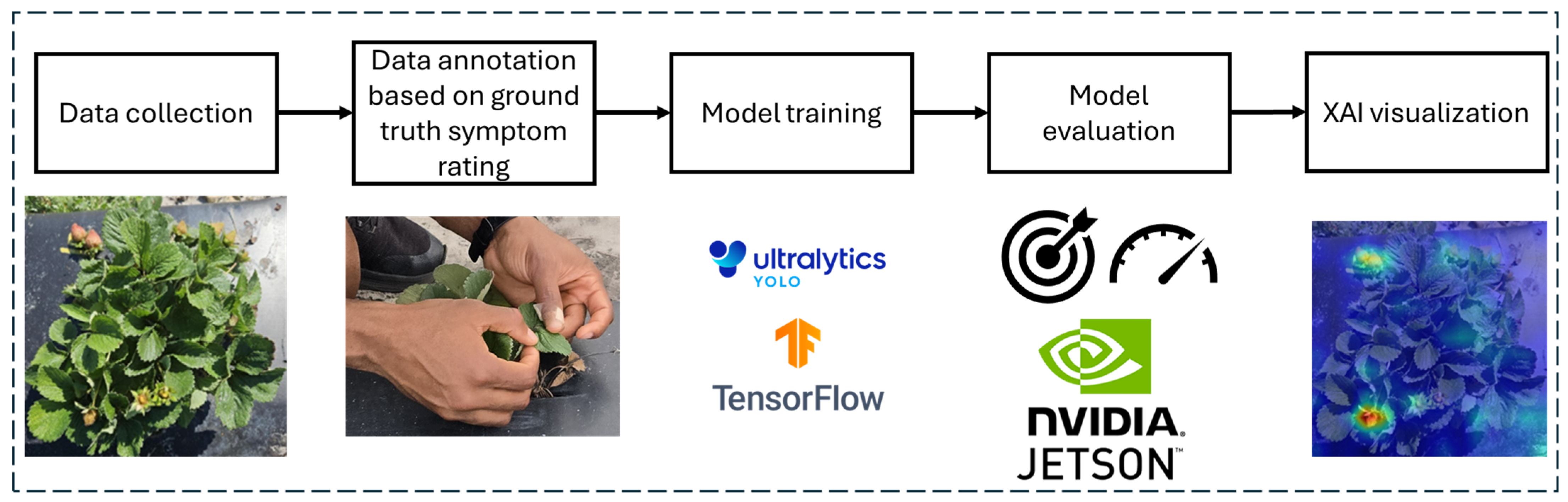
This study followed a five-stage experimental pipeline designed to develop and interpret a deep learning framework for estimating chilli thrips severity in strawberry plants (Figure 1). The workflow included (1) ground truth pest severity assessment and image collection of strawberry canopies under field conditions; (2) data annotation for three severity stages: healthy, moderately infested (moderate), and severely infested (severe) based on visible chilli thrips damage symptoms; (3) model training and benchmarking using multiple CNN architectures; (4) quantitative evaluation of classification performance and inference speed; and (5) application of XAI techniques to visualize the image regions most influential in model predictions.

2.1. Field Experiment Location and Layout

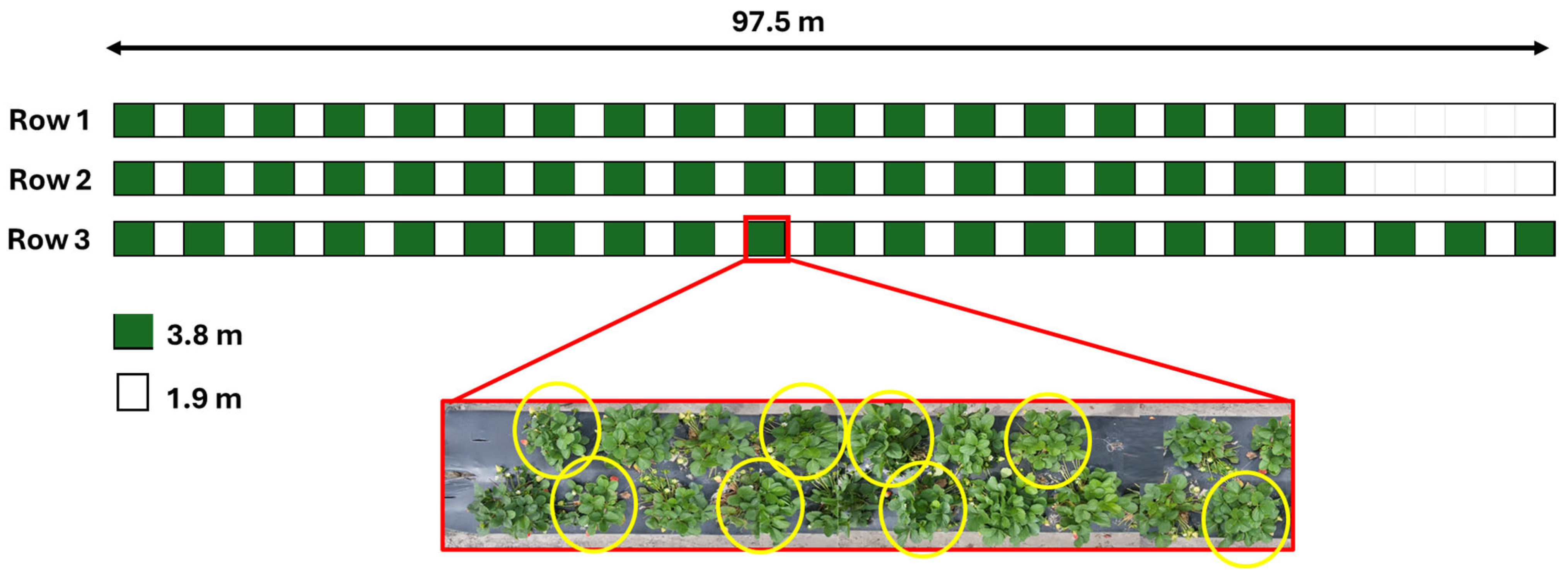
The field experiment was conducted using the ’Florida Brilliance’ strawberry cultivar plants [31], grown in raised beds covered with black polythene mulch at the University of Florida Gulf Coast Research and Education Center (UF GCREC, Wimauma, FL, USA, 27.76° N, 82.23° W). The experiment took place from October 2024 to March 2025, corresponding to one typical Florida strawberry production season. The field consisted of three double-planted rows of strawberry plants arranged in raised beds (Figure 2). Each row was divided into evenly spaced plots containing 20 plants each. The width of each plot was 3.8 m with 1.9 m buffer zones separating adjacent plots. Rows one and two contained 18 plots each, while row three contained 21 plots, resulting in a total of 57 plots and 1140 plants (57 plots × 20 plants per plot).

Standard commercial management practices were followed throughout the season [32], except that no insecticides were applied to allow natural chilli thrips infestation. Routine fungicide applications were maintained to prevent disease symptoms that could confound pest damage assessment. This management strategy ensured that observed foliar damage originated primarily from chilli thrips feeding rather than secondary pathogens or abiotic stress.

Eight plants from each plot (a total of 456) were randomly selected at the beginning of the season for continuous monitoring of pest symptom progression throughout the growing season. Visual scouting and image data collection were conducted weekly from 28 October 2024 to 3 March 2025. Figure 2 shows the field layout used for plant selection and image acquisition.

2.2. Data Collection

Data collection consisted of two sequential steps: (1) establishing the ground truth pest severity stage through visual plant analysis by trained experts, and (2) capturing RGB images of each plant canopy using smartphone cameras. This procedure was performed weekly for all 456 monitored plants throughout the production season.

2.2.1. Ground Truth Data Collection and Severity Estimation

Developing a reliable pest symptom severity classification model requires accurate ground truth data from trained experts. The ground truth severity stages were used to label the corresponding plant images. In Florida, Lahiri and Yambisa [7], and Adhikary et al. [33] categorized chilli thrips feeding symptoms on the youngest fully opened strawberry trifoliates into five stages (0 = no damage, 1 ≤ 10% trifoliate bronzing, 2 = between 10 and 30% trifoliate bronzing, 3 = between 31% and 60% of trifoliate bronzing, 4 ≥ 60% trifoliate bronzing). For this study, the five-stage expert scale was aggregated into three actionable classes explicitly aligned with integrated pest management (IPM) decision thresholds (

Table 1. Description of chilli thrips (Scirtothrips dorsalis) feeding symptom severity stages used for ground truth labeling of strawberry plants. The red circles indicate regions with symptoms of chilli thrips feeding and leaf necrosis.

Severity Stage	Description	Reference Image
Healthy	Clean trifoliate veins with little or no signs of necrosis at the base of the trifoliates and the mid-rib.
Moderately infested (moderate)	Clear signs of necrosis along most of the mid-rib extending to the lateral veins. The leaves show some signs of curling
Severely infested (severe)	Necrosis from feeding has extended to cover the entire trifoliate causing severe loss of chlorophyll (oily-like surface) and leaf curling.

). Predator releases are typically initiated when fields reach moderate symptom levels (stages 2–3), providing sufficient prey density for predator establishment, whereas stage 4 represents excessive damage and delayed intervention. Based on symptoms discussed in [7,33], the five expert-assigned stages were consolidated into three biologically and operationally meaningful categories. Healthy (stages 0–1) represented plants showing no or minimal bronzing, remaining below the action threshold for control measures. Moderate or action threshold (stages 2–3) encompassed plants exhibiting 10–60% bronzing, which corresponds to the typical intervention window for biological control, as predator releases are generally initiated within this range with sufficient prey density for predator establishment. Finally, severe (stage 4) denoted plants showing more than 60% bronzing, indicating late or uncontrolled infestations where interventions are often ineffective.

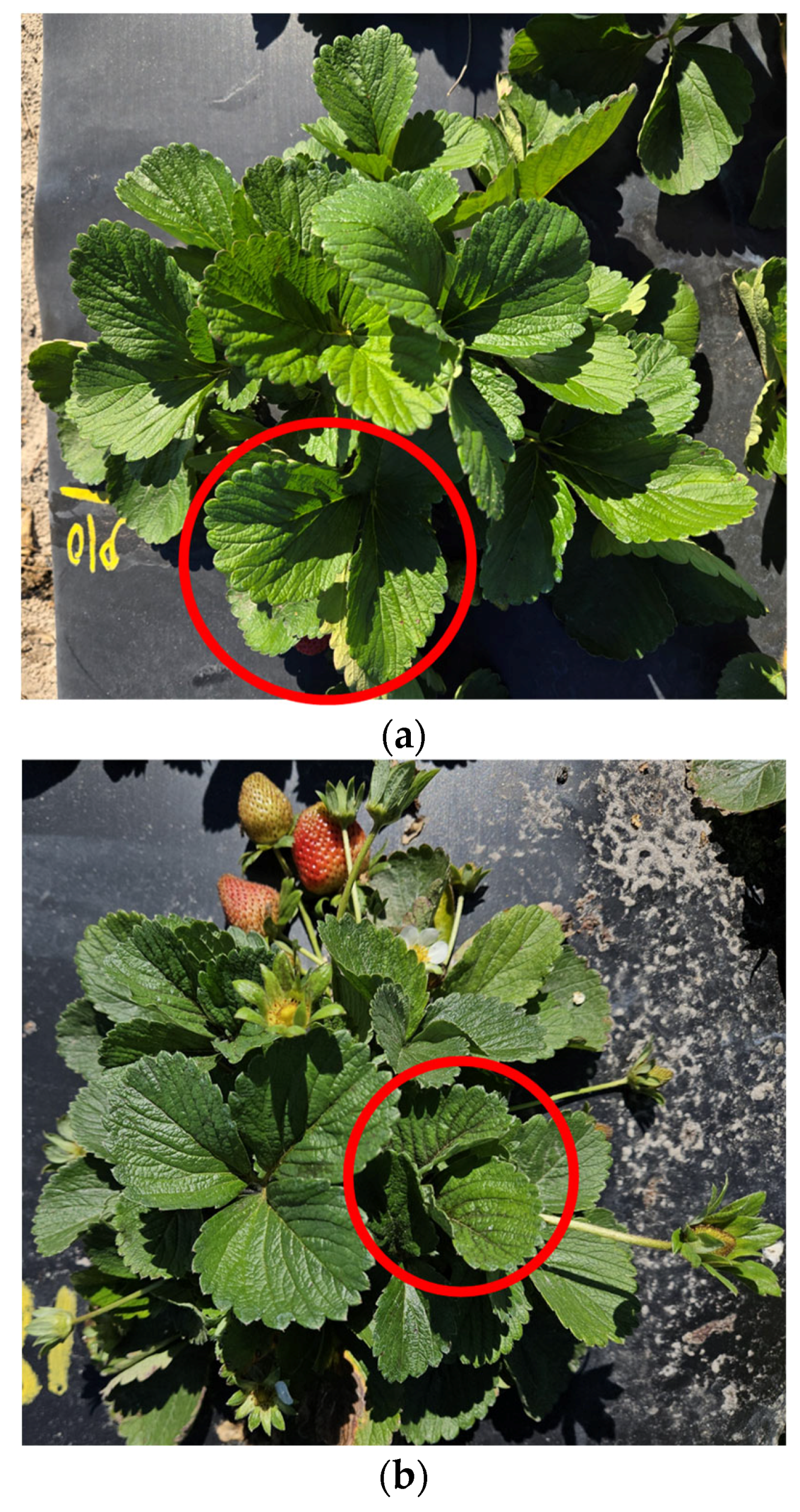
The visual plant analysis was conducted by manually inspecting the canopy of the plants, identifying the youngest fully opened trifoliates, and then assessing the spread of the necrosis (darkening of veins) from chilli thrips feeding. Based on the symptoms, the severity was classified into three stages: healthy, moderate, and severe.

2.2.2. Image Data Collection

Immediately after assigning the severity stage of a plant, a top-view RGB image of each plant canopy was captured. Each image was annotated using its corresponding ground truth label for model training. RGB images (JPEG and HEIC) were acquired under natural field lighting at various times of the day using either a Samsung smartphone (S10, S21 FE, S23+, and S24+, Samsung Electronics Co., Ltd., Suwon-si, Republic of Korea), or an Apple smartphone, (iPhone 13 and XR, Apple Inc., Cupertino, CA, USA) from a height of 0.2 m from the plant. The image resolution was approximately 3000 × 4000 pixels. After data collection and cleansing, 2135 images were retained from the 2024–2025 season, with 994, 994, and 147 for each respective stage. To mitigate class imbalance, 218 additional images captured at the end of the 2022–2023 growing season that showed plants with severe pest damage were added to the dataset for a total of 2353 images.

Table 2. Image acquisition dates for all severity stages.

Date	Healthy	Moderate	Severe	Total
16 March 2023			63	63
27 March 2023			155	155
28 October 2024	25			25
30 October 2024	31			31
5 November 2024	54			54
7 November 2024	32			32
12 November 2024	49	1		50
20 November 2024	109	1		110
27 November 2024	100	3	1	104
4 December 2024	94	4	1	99
12 December 2024	23			23
13 December 2024	37	2	1	40
18 December 2024	111	14	1	126
31 December 2024	114	87	1	202
27 January 2025	84	168	4	256
3 February 2025	75	183	14	272
17 February 2025	25	271	43	339
3 March 2025	31	260	81	372
Total	994	994	365	2353

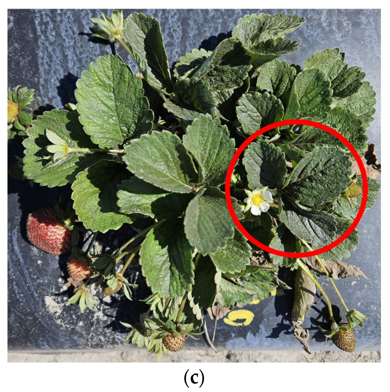
shows the date distribution of the images collected over the strawberry season, and Figure 3 shows example images acquired for each severity stage. All collected images were later standardized and augmented as described in Section 2.3.

2.3. Image Preprocessing and Data Augmentation

All image preprocessing was performed using the Roboflow computer vision development platform (Roboflow Inc., Des Moines, IA, USA, [34]). Each image was cropped to remove unnecessary background clutter and standardize the visible canopy region. Because chilli thrips severity progresses over time, the same plants were imaged repeatedly across the growing season as part of routine field monitoring. Consequently, individual plants transitioned through healthy, moderate, and severe stages as infestation advanced. This temporal progression was intentionally preserved to capture within-plant symptom evolution under field conditions. Image-level partitioning was therefore adopted to evaluate model performance under realistic temporal and phenological variability. Given the limited number of plants reaching the severe stage, a class-stratified sampling strategy was used to achieve sufficient representation of minority classes during evaluation. The training (33%) and validation (25%) subsets were constructed using an approximate 2:2:1 ratio (healthy: moderate: severe). The test subset (42%) followed the dataset’s natural prevalence (≈ 4.7:4.7:1), yielding 95 severe images to support statistically interpretable stage-wise evaluation (

Table 3. Train, validation, and test data partitioning.

Stage	Train	Percent	Validation	Percent	Test	Percent	Total
Healthy	308	0.31	232	0.23	454	0.46	994
Moderate	308	0.31	232	0.23	454	0.46	994
Severe	154	0.42	116	0.32	95	0.26	365
Total	770	0.33	580	0.25	1003	0.42	2353

). This allocation provides a conservative assessment of field performance while maintaining adequate training diversity through transfer learning from ImageNet-pretrained backbones. A larger test set was intentionally retained to evaluate robustness across variable lighting, canopy maturity, and device types encountered in field operations. Table 3 breaks down the data partitioning strategy. To enhance model generalization, the training set images were augmented threefold (Roboflow API) by applying random transformations, including horizontal and vertical flips, 90-degree rotations (clockwise, and counterclockwise), saturation (−15% to 15%), exposure (−10% to 10%), crop (0% to 10% zoom), and salt-and-pepper noise (up to 0.22% of pixels) to the images.

2.4. Classification Models

This study implemented transfer learning with pretrained weights from four classic CNN architectures: You Only Look Once (YOLOv11) [35], EfficientNetV2 [36], Xception [37] and MobileNetV3 [38]. These architectures were selected for their proven ability to effectively balance computational efficiency and accuracy through improved spatial attention while minimizing parameter size.

YOLO models are widely used due to their ease of implementation in resource-constrained object detection tasks. However, there is limited information about YOLO models for fine-grained multiclass image classification problems (classification of subcategories, e.g., types of birds, car models, etc.). The EfficientNetV2 and Xception architectures are common for developing highly accurate and robust image classification models. However, these models can be computationally expensive with large parameter counts, causing reduced performance in resource-constrained applications. The MobileNetV3 model, built for lightweight mobile phone CPUs, has the lowest parameter count of all the models. However, the lower parameter count can result in lower accuracy in image classification problems.

These four model architectures represent a spectrum of trade-offs between model size (small to large), accuracy (low to high), and inference speed (high to low), key considerations for real-time pest severity classification and on-device deployment in field environments.

2.4.1. Model Parameters

Models were trained using square images of sizes 256, 480, 640, and 1024 pixels to evaluate trade-offs between computational efficiency and prediction accuracy with varying levels of visual detail. Preliminary hyperparameter tuning was conducted to determine the optimal learning rate and optimizer combinations. As performance remained consistent across configurations, the learning rate was kept between 0.0001 and 0.00147, with the adaptive moment estimation with weight decay (AdamW) optimizer.

Table 4. Model training parameters.

Parameter	Value
Patience	25
Optimizer	AdamW
Learning Rate	0.0001 to 0.00147
Learning Rate for Finetuning	0.1 × Learning Rate
Dropout Rate	0.3
Batch Size	16
Epochs	100
Finetuning Epochs	20
Number of layers for finetuning (YOLO)	2
Number of layers for finetuning (others)	40

summarizes the parameters used for training the classification models. Model training was performed using the University of Florida Hipergator 3.0 research computing cluster (UFIT Research Computing, Gainesville, FL, USA). The computing node consisted of eight AMD EPY 7742 Rome cores, 2 NVIDIA Ampere A100 GPUs (80 GB each), and 64 GB of system memory. Small-, medium-, and large-sized model weights were tested for the YOLOv11 and EfficientNetV2 families, while only the large-sized weights of the MobileNetv3 family were tested. All the selected models achieved accuracy scores greater than 75% with parameter sizes between 5.4 M to 54.4 M on the ImageNet benchmark dataset [39]. The YOLO models were implemented using the PyTorch framework (Torch 2.4, Linux Foundation, San Francisco, CA, USA) with CUDA 12.6 (NVIDIA Corporation, Santa Clara, CA, USA) and the Ultralytics package, while the remaining models were implemented with the TensorFlow Keras framework (TensorFlow 2.16, Google, Mountain View, CA, USA).

2.4.2. Transfer Learning and Finetuning

To accelerate convergence and improve feature generalization, all models were initialized with ImageNet [39] pretrained weights. All models were trained for 100 epochs, with early stopping implemented based on the validation accuracy with a patience threshold of 25 epochs, i.e., if the validation accuracy did not improve after 25 epochs, model training was stopped. Following convergence, the best weights were saved. The model weights were subsequently finetuned by unfreezing the last few layers before the classification head (2-layer blocks for YOLO; 40 layers for EfficientNetV2, Xception, and MobileNetV3). Then, finetuning continued for an additional 20 epochs using a smaller learning rate and patience of 10 epochs to refine high-level representations without overfitting (Table 4). The best-performing model weights were automatically saved based on validation performance.

2.5. Inference on Edge Device

To evaluate real-time deployment feasibility, the trained models were benchmarked on an edge device: an NVIDIA Jetson Orin Nano 8 GB Module (CPU: 6-core Arm, GPU: NVIDIA Ampere with 1024 CUDA cores and 32 tensor cores, NVIDIA Corporation, Santa Clara, CA, USA). The trained weights were converted from their respective framework formats into the TensorRT engine format (TensorRT 10.3, NVIDIA Corporation) for optimized low-latency inference. Conversion was performed through the Open Neural Network Exchange (ONNX 1.17, opset 17, ONNX Contributors, 2024). This conversion process was required for compatibility across architectures and minimized computational overhead during real-time classification. Inference was run on a batch size of 12 images with full precision (fp32) inference to prioritize a balance between high-throughput and high accuracy execution on the edge device. The inference latency was calculated using the total processing time, comprising image preprocessing, model inference, and postprocessing. The average batch processing time was divided by the batch size to estimate per-image latency (ms), and throughput was subsequently calculated in images per second (images/s).

2.6. System Performance Evaluation Metrics

Model performance was evaluated using multiple quantitative and qualitative metrics to capture both predictive accuracy and practical utility for pest management applications. The primary metric used for model evaluation was the test set top-1 accuracy (Equation (1)), defined as the ratio of the number of correct predictions to the size of the test dataset. Since the dataset consisted of three classes, top-1 accuracy ensured that model priority is given to only the class with the highest confidence. While this metric is widely used to assess overall classification performance, it can be misleading in cases of class imbalance. In this study, the number of healthy and moderate stage images was approximately five times higher than that of the severe stage (4.7:4.7:1). Therefore, additional metrics were introduced to provide a more balanced evaluation. To account for the uneven class distribution, the macro-average recall (Mac-R, Equations (2) and (3)) was calculated. This metric computes the recall (true positive rate) for each class independently and then averages them, ensuring that equal weight is given to each class regardless of its frequency. Mac-R thus provides a more representative assessment of model performance across all severity stages.

From a pest management perspective, it is important to minimize false negatives, the situations where the model predicts a moderate or severe stage plant as a healthy stage plant. Such errors delay intervention, allowing pest populations to establish and potentially cause significant economic losses. To evaluate this risk, confusion matrices were analyzed, and the false positive rates (FPRs, Equation (4)) for the healthy class were used as an additional indicator of model robustness. A lower FPR for the healthy class implies fewer missed detections of moderate or severe infestations, even if this results in more false positive predictions for infested plants.

For real-time field deployment, computational performance was also assessed using the average inference time (ms), and throughput (image/s) measured on the NVIDIA Jetson Orin device.

$$\mathrm{Top}\text{-}1 \mathrm{Accuracy}={\displaystyle \frac{1}{N}}{\displaystyle \sum }_{i=1}^{N}I(\widehat{y_i}{=y}_i)$$

(1)

$$\mathrm{Recall}={\displaystyle \frac{\mathrm{TP}}{\mathrm{TP}+\mathrm{FN}}}$$

(2)

$$\mathrm{Mac}\text{-}\mathrm{R}={\displaystyle \frac{{\mathrm{Recall}}_a{+\mathrm{Recall}}_b+\dots {\mathrm{Recall}}_K}{K}}$$

(3)

$${\mathrm{FPR}}_{\mathrm{healthy}}={\displaystyle \frac{{\mathrm{FP}}_{\mathrm{healthy}}}{{\mathrm{FP}}_{\mathrm{healthy}}{+\mathrm{TN}}_{\mathrm{healthy}}}}$$

(4)

where N = number of images in the test dataset,

• $\widehat{y_i}$ = predicted label,
• $y_i$ = true label,
• TP = true positives,
• FP = false positives,
• FN = false negatives,
• TN = true negatives,
• FPR = false positive rate,
• Mac-R = macro-average recall,
• K = number of classes.

2.7. Grad-CAM XAI for Model Explanation

To interpret the visual features that strongly influenced model decisions, the Gradient-Weighted Class Activation Mapping (Grad-CAM) [40] technique was used. Grad-CAM enables visualization of spatial regions within an image that contribute most to model classification outcomes, thereby transforming an otherwise opaque convolutional network into a more interpretable diagnostic tool. The Grad-CAM procedure was applied to the best-performing model configuration with the highest top-1 accuracy, YOLO11m-cls trained with 1024 by 1024-pixel input image size (Section 3). With this method, a test image was fed through the model, and the gradients between the predicted output class $c$, $y^c$, with respect to the feature maps, $A_{i,j}^k$, in the last convolutional layer (model[10].conv) were computed. These gradients were spatially averaged to obtain neuron importance weights, ${\mathsf{\alpha }}_k^c$ (Equation (5)), representing the contribution of each feature map channel $k$ to the class prediction. The Grad-CAM heatmap, $L_{\mathrm{Grad}\text{-}\mathrm{CAM}}^c$ (Equation (6)), was then obtained as a weighted linear combination of the activation maps for class $c$. 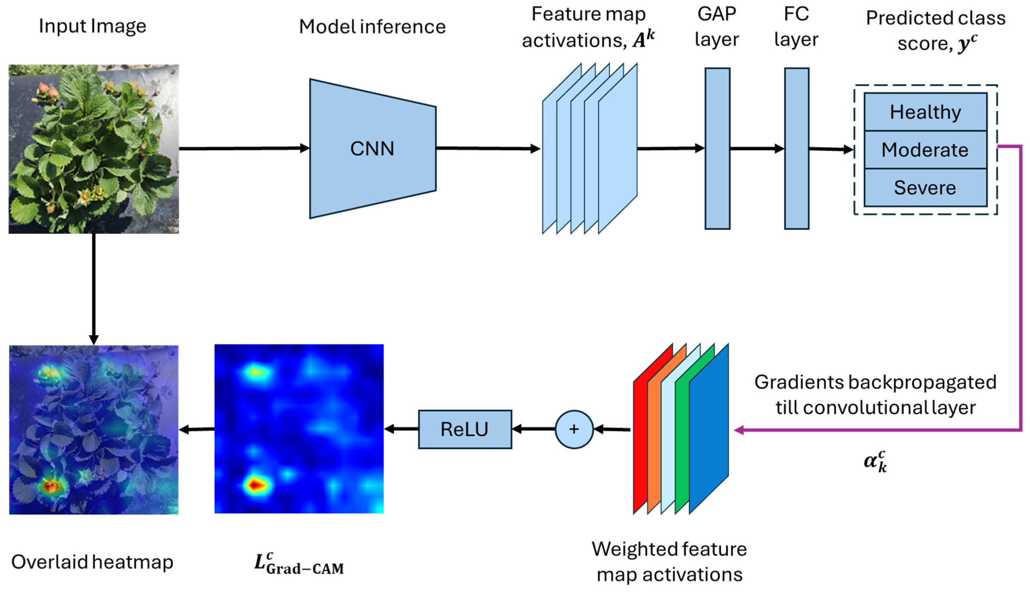Then, a Rectified Linear Unit (ReLU) activation was applied to suppress negative gradients and highlight features with a positive influence on the predicted class. The resulting heatmap was then overlaid on the original RGB image to visualize key regions that guided model decisions (Figure 4). This approach allowed examination of attention differences across three classes, healthy, moderate, and severe, for the same image, regardless of the final output label. Such visualizations aid in interpreting misclassifications or low-confidence predictions by revealing overlapping visual cues between symptom stages. From a biological standpoint, Grad-CAM heatmaps helped identify canopy-level plant regions correlated with chilli thrips symptoms beyond the hidden young trifoliates, such as leaf curling or discoloration on fruits and leaves that may serve as early diagnostic indicators before visible trifoliate bronzing occurs. These insights are critical for guiding future dataset refinement and model retraining to improve both robustness and biological validity. Grad-CAM was implemented using the pytorch-grad-cam 0.2.1 library [41].

$${\mathsf{\alpha }}_k^c={\displaystyle \frac{1}{Z}}{\displaystyle \sum }_i{\displaystyle \sum }_j{\displaystyle \frac{\partial y^c}{\partial A_{i,j}^k}}$$

(5)

$$L_{\mathrm{Grad}\text{-}\mathrm{CAM}}^c=\mathrm{ReLU}\left({\displaystyle \sum }_k{\mathsf{\alpha }}_k^c{A}^k\right)$$

(6)

where ${\mathsf{\alpha }}_k^c$ = neuron importance weight for feature map k with respect to class c,

• c = class,
• k = feature map channel,
• Z = size of feature map (height × width),
• i, j = width and height dimensions,
• $y_c$ = logit for class c,
• $A_{i,j}^k$ = activation value at i, j, in feature map k,
• $L_{\mathrm{Grad}\text{-}\mathrm{CAM}}^c$ = final Grad-CAM heatmap.

Figure 4. Overall schematic of the Grad-CAM framework used in this study. The image is forward propagated to obtain prediction scores for each class. The gradients (${\mathsf{\alpha }}_k^c$) from any of the classes are backpropagated to the last convolutional layer (before the global average pooling and fully connected layers) to obtain a weighted feature map that is overlaid on the original image to visualize the relevant spatial regions.

Figure 4. Overall schematic of the Grad-CAM framework used in this study. The image is forward propagated to obtain prediction scores for each class. The gradients (${\mathsf{\alpha }}_k^c$) from any of the classes are backpropagated to the last convolutional layer (before the global average pooling and fully connected layers) to obtain a weighted feature map that is overlaid on the original image to visualize the relevant spatial regions.

To quantitatively assess model attention patterns, Grad-CAM heatmaps were analyzed using a region-based and entropy-based framework. For each severity class (healthy, moderate, and severe), ten representative images were selected based on high prediction confidence to provide stable and interpretable activation patterns. Limiting the analysis to a small, representative subset allowed consistent region-based and entropy-based comparisons while maintaining interpretability. Grad-CAM heatmaps were generated from the final convolutional layer of the classification network and normalized to the range [0, 1]. A fixed activation threshold (τ = 0.8) was applied to identify high-activation regions, with pixels exceeding this threshold considered highly informative for the model’s prediction. To associate model attention with biologically meaningful plant structures, each image was paired with a corresponding semantic mask comprising five regions: background, leaves, fruits, flowers, and stems. The proportion of high-activation pixels overlapping each region, $pr$ was computed as Equation (7).

$$pr={\displaystyle \frac{\left|A_{\mathsf{\tau }}\cap R_r\right|}{A_{\mathsf{\tau }}}}$$

(7)

where $A_{\tau }$ denotes the set of high-activation pixels and $R_r$ denotes pixels belonging to region $r$. These proportions were computed at the image level and averaged within each severity class to obtain class-level region-based attention statistics.

Attention dispersion was quantified using Shannon entropy, calculated from the region-wise activation proportions (Equation (8)).

$$H={\displaystyle \sum }_{r}pr \log (pr+ϵ)$$

(8)

where $ϵ$ is a small constant added to avoid numerical instability. Lower entropy values indicate localized attention concentrated on specific regions, whereas higher values indicate diffuse attention distributed across multiple regions.

In addition, high-activation spatial coverage was computed as the ratio of high-activation pixels to the total number of image pixels. This metric captures the spatial extent of model attention and distinguishes localized feature reliance from canopy-wide activation patterns. All quantitative metrics (region proportions, entropy, and coverage) were summarized using mean and standard deviation for each severity class and used to complement qualitative Grad-CAM visualizations.

3. Results and Discussion

3.1. Model Classification Results

Transfer learning with frozen pretrained weights and dropout layers significantly reduced training convergence time while resulting in consistently higher accuracies across all architectures. As all pretrained backbones performed comparably on the ImageNet dataset, the top-1 accuracies for the chilli thrips classification dataset were within the range of 77–85%.

Table 5. Comparison of model architectures, parameter sizes, input image resolutions, and performance metrics for chilli thrips pest severity classification.

Model Weights	Params (M)	Image size (Pixel)	Train Acc (Top-1)	Val Acc (Top-1)	Test Acc (Top-1)	Macro Avg Recall	FPR Healthy	Speed (ms/ Image)	Average Throughput (Image/s)	Accuracy-to-Speed Ratio
YOLO11s-cls.pt 1	5.5	256	89.3%	79.7%	81.6%	81.7%	7.7%	8.9	112	0.092
		480	87.0%	81.4%	83.2%	84.3%	9.1%	13.6	73	0.061
		640	82.0%	83.3%	83.3%	83.2%	14.4%	18.0	55	0.046
		1024	91.8%	83.1%	83.5%	83.7%	13.5%	38.6	25	0.022
YOLO11m-cls.pt 1	10.4	256	85.7%	79.3%	82.5%	81.3%	12.2%	10.7	93	0.077
		480	85.7%	81.4%	82.6%	83.0%	8.7%	19.3	51	0.043
		640	93.7%	81.2%	82.3%	82.8%	9.1%	29.0	34	0.028
		1024	90.8%	82.9%	84.8%	84.7%	9.5%	70.7	14	0.012
YOLO11x-cls.pt 1	28.4	256	83.9%	80.2%	81.7%	80.7%	7.8%	15.0	66	0.055
		480	90.6%	80.5%	82.0%	82.0%	7.3%	43.7	22	0.019
		640	88.3%	83.3%	81.7%	82.3%	6.9%	62.1	16	0.013
		1024	90.0%	82.9%	83.2%	83.2%	17.3%	160.7	6	0.005
EfficientNetV2B0	7.2	256	79.0%	76.7%	80.4%	82.5%	18.2%	5.7	176	0.142
		480	82.9%	82.1%	81.2%	82.8%	19.9%	10.8	92	0.075
		640	80.7%	80.5%	80.8%	81.7%	19.9%	16.0	62	0.051
		1024	80.4%	81.4%	83.0%	83.3%	18.4%	33.1	30	0.025
EfficientNetV2B3	14.5	256	73.9%	83.1%	79.8%	79.5%	7.3%	10.0	99	0.080
		480	77.1%	82.8%	80.4%	80.5%	8.0%	28.3	35	0.028
		640	73.2%	84.5%	81.1%	79.7%	5.5%	47.5	21	0.017
		1024	78.0%	85.2%	82.1%	82.1%	6.7%	128.3	7	0.006
EfficientNetV2S	21.6	256	74.6%	81.0%	80.2%	79.0%	8.6%	13.8	72	0.058
		480	79.1%	83.1%	81.8%	82.7%	7.8%	39.5	25	0.021
		640	77.2%	85.2%	82.4%	83.4%	8.6%	67.6	14	0.012
		1024	79.1%	83.4%	82.1%	82.3%	6.6%	171.5	5	0.005
EfficientNetV2M	54.4	256	81.3%	77.8%	77.2%	79.3%	13.8%	22.4	44	0.034
		480	74.0%	84.8%	78.6%	72.3%	6.2%	58.5	17	0.013
		640	76.1%	80.9%	80.6%	80.4%	8.6%	119.0	8	0.007
		1024	76.8%	86.9%	81.7%	80.1%	7.8%	262.3	3	0.003
Xception	22.9	256	73.8%	81.0%	78.0%	75.7%	8.9%	12.0	83	0.065
		480	84.5%	83.4%	80.7%	81.6%	8.4%	34.6	28	0.023
		640	82.2%	84.8%	81.2%	81.4%	11.3%	58.1	17	0.014
		1024	78.0%	84.5%	82.0%	82.3%	8.9%	155.3	6	0.005
Mobile-NetV3Large	5.4	256	71.6%	78.4%	78.1%	79.4%	11.8%	6.5	153	0.120
		480	75.5%	80.9%	83.2%	83.4%	9.3%	12.2	82	0.068
		640	78.3%	80.2%	81.4%	81.8%	4.2%	20.6	48	0.039
		1024	75.5%	80.5%	82.2%	82.7%	10.0%	57.8	17	0.014

¹ YOLO models began overfitting to the training data despite regularization measures. Bold values represent the best performance for each metric.

summarizes the results for all model architectures, parameter sizes, input image resolutions, and performance metrics for chilli thrips damage severity classification. Despite the addition of dropout layers and early stopping regularization to mitigate overfitting, some models showed mild divergence between training and validation sets. In some cases, training accuracy appeared lower than validation accuracy because dropout and batch normalization layers behave differently during training and evaluation. During training, dropout was active and batch normalization relied on mini-batch statistics, which can introduce additional stochasticity and reduce training accuracy. During validation and testing, dropout was disabled and batch normalization used accumulated running statistics, often resulting in higher and more stable accuracy estimates. This behavior is a well-known regularization effect rather than an indication of model underperformance [42]. Model evaluation was conducted using the test set, which contained the most images across all splits (n_train = 770, n_val = 580, n_test = 1003), for statistical reliability.

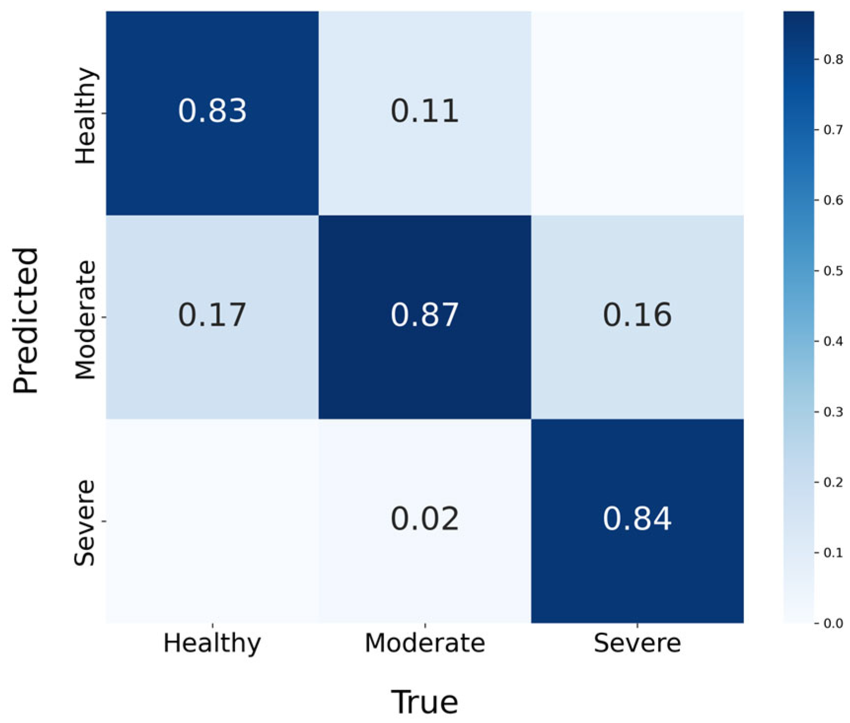
Most of the trained models achieved a test set top-1 accuracy greater than 80%, confirming that all four tested CNN families, YOLOv11, EfficientNetV2, Xception and MobileNetV3, were capable of distinguishing chilli thrips damage severity stages from canopy-level RGB imagery. Among all model weights and image size configurations, the YOLO11m-cls with 1024-pixel input image resolution achieved the highest performance with a top-1 test accuracy of 84.8%, and a macro-average recall (Mac-R) of 84.7%, marginally outperforming other architectures. Stage-wise accuracies reached 83%, 87%, and 85%, respectively, for healthy, moderate, and severe stages (Figure 5 and

Table 6. Stage-wise metrics for YOLO11m-cls and 1024-pixel model configuration.

Stage	Precision	Recall	F1-Score
Healthy	87.9%	83.0%	85.4%
Moderate	81.1%	86.8%	83.8%
Severe	90.9%	84.2%	87.4%
Macro-average	86.6%	84.7%	85.6%

).

From a practical perspective, all misclassifications occurred between adjacent classes. As shown in Figure 5, about 17% of healthy plants were misclassified as moderate, and 11% of moderate plants were predicted as healthy; cross-extreme errors such as severe class plants being misclassified as healthy plants were not found. Among these, the most critical error for pest management is when moderate infestations were misclassified as healthy (11%), as such false negatives could delay intervention and allow thrips populations to increase. In contrast, healthy-to-moderate misclassification (17%) mainly results in precautionary monitoring or early scouting, which has minimal biological or economic consequences. Therefore, maintaining a low false-negative rate for the healthy class is the most important criterion for providing operational reliability of canopy-level severity prediction systems.

Overall, the Mac-R values appeared within 1 to 2 percent of the top-1 accuracies for all models (Table 5). This suggests that all trained models generalized well for all classes, including the severe class with a significantly lower sample size (n = 95). The only exception was the EfficientNetV2M model with 480-pixel image size, which showed a 6% drop in Mac-R relative to the top-1 accuracy, suggesting overfitting or limited class representation. From the analysis, the highest top-1 accuracy configuration (YOLO11m-cls and 1024-pixel) also achieved the highest Mac-R score (84.7%) and was the most robust model for classifying the pest severity stages.

In pest management contexts, false negatives, cases where moderate or severe infestations are predicted as healthy, are particularly detrimental because they delay intervention. Thus, the false positive rate (FPR) for the healthy class was analyzed as a reliability metric. From analyses of the confusion matrices, all models achieved FPR scores lower than 18% for all image size configurations. The MobileNetV3Large and 640-pixel combination scored the best with just 4.2%. The best-performing model, YOLO11m-cls with 1024-pixel input image size, also achieved a satisfactory performance with an FPR of 9.5%.

3.2. Trade-Offs Between Accuracy, Speed, Image Size and Parameter Count

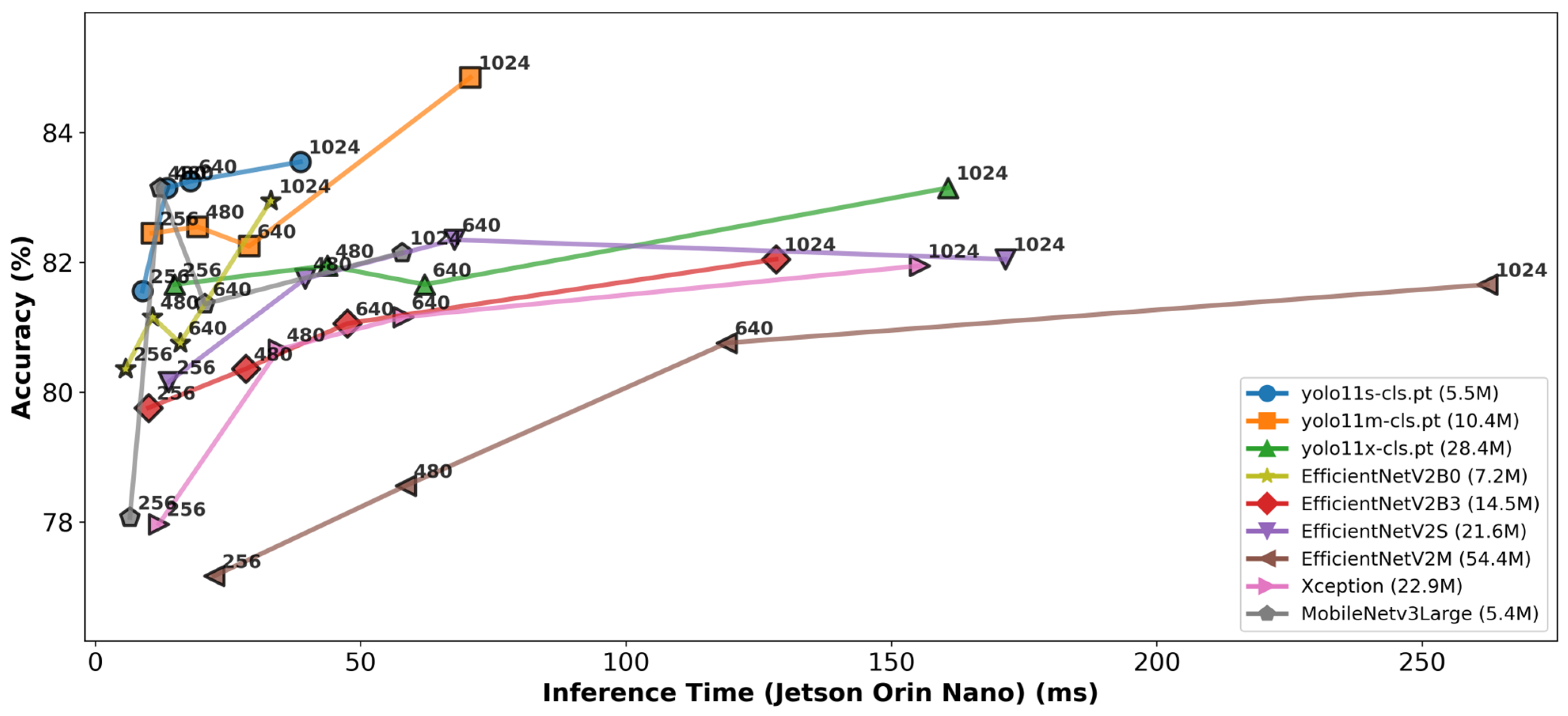
The trade-off between model accuracy and inference time is illustrated in Figure 6. As expected, models with larger parameter counts and input image sizes correspond to slower inference speed. The initial hypothesis was that larger image sizes would yield higher accuracy scores because they preserve detailed visual cues and are capable of spotting subtle chilli thrips symptoms such as vein bronzing, necrotic specks, and leaf curling (Table 1 and Figure 3). 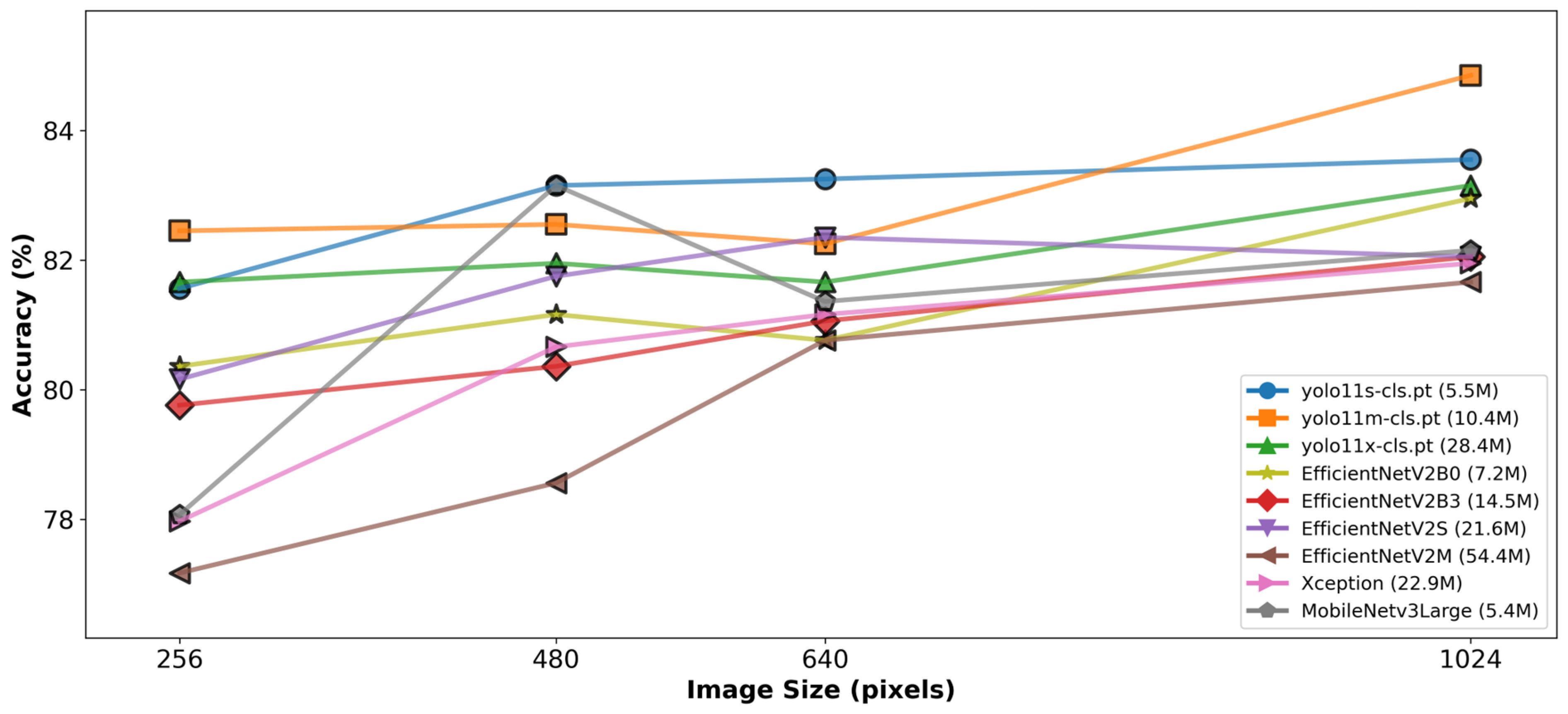As shown in Table 5 and Figure 7, increasing input image resolution generally improved classification accuracy with gains of approximately 2–5% between the lowest (256-pixel) and highest (1024-pixel) resolutions. This reflects the availability of more discriminative details at larger pixel scales. However, the improvement was not strictly proportional to image size; accuracies tended to plateau beyond 640-pixel resolution and, in some cases, slightly decline, possibly due to overfitting. This suggests that beyond a certain resolution, additional contextual information contributes only marginally to discriminative learning while substantially increasing computational burden. Furthermore, because the dataset size was relatively limited, some architectures may have overfit due to image-specific noise or background artifacts, resulting in a steeper rise in training accuracy compared to validation performance.

In contrast, three lightweight models with the smallest parameter sizes, YOLO11s-cls (5.5 M), MobileNetV3Large (5.4 M), and EfficientNetV2B0 (7.2 M) reached up to 83% top-1 accuracy and 83% Mac-R, exhibiting comparable or higher validation accuracy while maintaining faster convergence and better generalization. Meanwhile, the EfficientNetV2M model, despite having 10 times the number of parameters (54.4 M), achieved 81.7% peak top-1 accuracy and 80.1% Mac-R for the 1024-pixel image size, indicating diminishing returns from deeper and heavier architectures under limited training data. Therefore, a balance between visual detail and computational efficiency must be maintained when selecting optimal image resolutions for real-time deployment. The compact architectures, combined with efficient attention mechanisms (such as C2PSA block for YOLOv11, and Squeeze-and-Excitation block for MobileNetV3 and EfficientNetV2), potentially allowed the models to capture the key canopy-level texture and color cues associated with chilli thrips injury without excessive parameter overhead.

The added benefit of a lower parameter count and smaller image sizes is their substantially faster inference time. In Figure 6, most data points fall in the top left quadrant, demonstrating that most model weights and image size configurations achieved high accuracy while maintaining low latency for this experiment. The EfficientNetV2B0 baseline model with a relatively small number of parameters exhibited the fastest performance and accuracy-to-speed ratio, processing images in less than 6 ms (176 image/s throughput) with up to 80% top-1 accuracy.

In standard image classification tasks, the goal is to minimize a loss function, and, consequently, the number of misclassified images across different classes with improved generalizability for unseen datasets. With these criteria, the highest accuracy model- YOLO11m-cls (1024-pixel) can be considered as the benchmark model for offline inference. However, from an application standpoint, this trade-off between accuracy and speed is critical. In resource-constrained real-time pest management, real-time feedback enables rapid pest detection and decision-making. While YOLO11m-cls achieved the highest test accuracy among the evaluated configurations and was therefore selected for detailed analysis, other models demonstrated strong and complementary performance profiles. Particularly, EfficientNetV2B0 and YOLO11s-cls offered competitive accuracy with fewer parameters and faster inference speeds, showing that the choice of model depends on application-specific constraints rather than accuracy alone. Conversely, larger architectures, such as EfficientNetV2M and YOLO11x-cls, achieved only marginal accuracy gains while requiring more than 150 ms per inference, limiting their suitability for real-time deployment on embedded platforms.

On a final note, while YOLO models are widely used for traditional object detection and localization tasks, there is still limited research about YOLO models for fine-grained image classification. In this investigation, the YOLO classification models performed comparably to the other tested models that are known primarily for rich feature extraction, demonstrating the potential for YOLO-based models as effective backbones for future real-time agricultural image classification tasks.

3.3. Real-Time Inference Performance Evaluation

The optimized models were deployed on the NVIDIA Jetson Orin Nano (8 GB) to evaluate inference performance on an embedded edge device. The edge device obtained comparable test set accuracies to those of the A100 training GPUs, indicating that the ONNX and TensorRT conversion framework effectively preserved model accuracy while significantly improving computational efficiency. In general, devices with throughput values greater than 20 image/s (or inference times below 50 ms/image) are considered suitable for real-time applications [43,44,45]. Within this threshold, the YOLO11s-cls, EfficientNetV2B0 and MobileNetV3Large configurations demonstrated particularly strong performance, balancing high accuracy with fast processing speeds. This performance is critical for closed-loop pest management systems, such as the predatory mite dispensing platform under development, where rapid image processing is required to guide actuator responses and avoid bottlenecks in field operation. Most of the tested models satisfied the real-time criteria for image sizes of 256-pixel, 480-pixel, and 640-pixel while maintaining high accuracies and Mac-R scores. Only at 1024-pixel resolution did inference time fail to meet real-time thresholds, suggesting that while a higher resolution marginally benefits classification accuracy, it may hinder operational feasibility in time-sensitive agricultural robotics contexts.

Table 7. Model selection decision table.

Objective	Recommended Model	Input Size	Accuracy	Latency (ms)	FPS	Comments
Maximum accuracy and generalization	YOLO11m-cls.pt	1024 × 1024	84.8%	70.7	14	For offline or near-real-time diagnosis
Real-time application	EfficientNetV2B0	256 × 256	80.4%	5.7	176	For continuous scouting in resource-constrained applications
Lowest missed detections	MobileNetV3Large	640 × 640	81.4%	20.6	48	For complete pest reduction scenarios where missed infestations are costly

details model and input image resolution recommendations for applications with different priorities including maximum accuracy, real-time efficiency, and reduced missed detections.

3.4. Feature Visualization Using Grad-CAM

While numerical metrics validate model performance, they do not reveal how the networks make decisions or what visual cues drive predictions. To bridge this gap, Grad-CAM, an XAI technique, was employed to visualize and interpret model reasoning, providing transparency and biological interpretability in pest severity estimation.

3.4.1. Key Features Driving Model Predictions

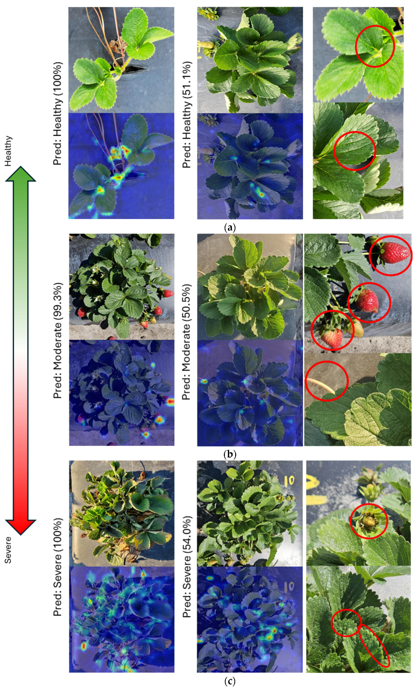
Figure 8 shows Grad-CAM visualizations for healthy, moderate, and severe chilli thrips severity stage predictions. The heatmaps reveal that model attention was not random, but concentrated on distinct canopy regions, primarily fruits (mature, immature, or senescing), stems (healthy or dying), flowers, trifoliate intersection, and leaf edges, indicating that the network developed an implicit understanding of biologically meaningful structures. Although Grad-CAM does not explicitly identify what visual attributes the model learned (e.g., color variance, texture deformation, or geometric irregularity), it effectively highlights where the discriminative evidence resides within each image.

For healthy stage classifications (Figure 8a), Grad-CAM tended to focus on narrow regions, typically at the leaf trifoliate intersection (the junction where the three leaflets meet the petiole), an area that typically remains structurally intact and uniformly pigmented under non-infested conditions. This attention likely reflects model recognition of features that correspond to the absence of feeding damage defined in the ground truth in Section 2.2.1 (Table 1). The network thus appears to use this geometrically stable region as a visual anchor for identifying normal canopy structure, suggesting that its learned representations are both interpretable and physiologically relevant. Moderate stage heatmap activations shifted toward fruits, where thrips feeding causes cracking and bronzing (Figure 8b). These areas often display subtle irregularities such as texture roughness or localized pigment loss that the model possibly detected as deviations from the “healthy baseline”. The correspondence between these highlighted regions and the biological feeding sites reported by Kumar et al. [3], Lahiri & Yambisa [7], and Adhikary et al. [33] demonstrates that the CNN may have internalized biologically meaningful progression patterns. In the severe stage, Grad-CAM heatmaps (Figure 8c) became highly diffuse, covering entire trifoliates, senescent fruits, and necrotic stems. This pattern aligns with the terminal ground truth category (Table 1) and indicates that the model recognized the global breakdown of structural coherence, such as extreme curling, chlorophyll depletion, and tissue collapse, as characteristics of advanced thrips injury. The broad highlighted regions scattered around the heatmap also suggest that the network no longer relies solely on localized features once the overall structural organization of the canopy deteriorates.

These Grad-CAM–ground truth associations imply that the CNN has implicitly learned a visual continuum of symptom development, progressing from structural order to disorder. Importantly, the model’s early attention shifts, from the trifoliate junction (healthy) to fruits with feeding signs (moderate), corresponding to the critical intervention window for predatory mite release between healthy and moderate stages of the ground truth framework. This suggests that Grad-CAM visualization can serve not only as an interpretability tool but also as a biologically informed decision aid, helping define threshold imagery that signals when biological control should be deployed. Future work should explore using aggregated Grad-CAM attention statistics as quantitative indicators of pest pressure, enabling a dynamic, explainable link between AI classification output and actionable integrated pest management (IPM) decisions.

3.4.2. Sources of Misclassifications and Lower Confidence Scores

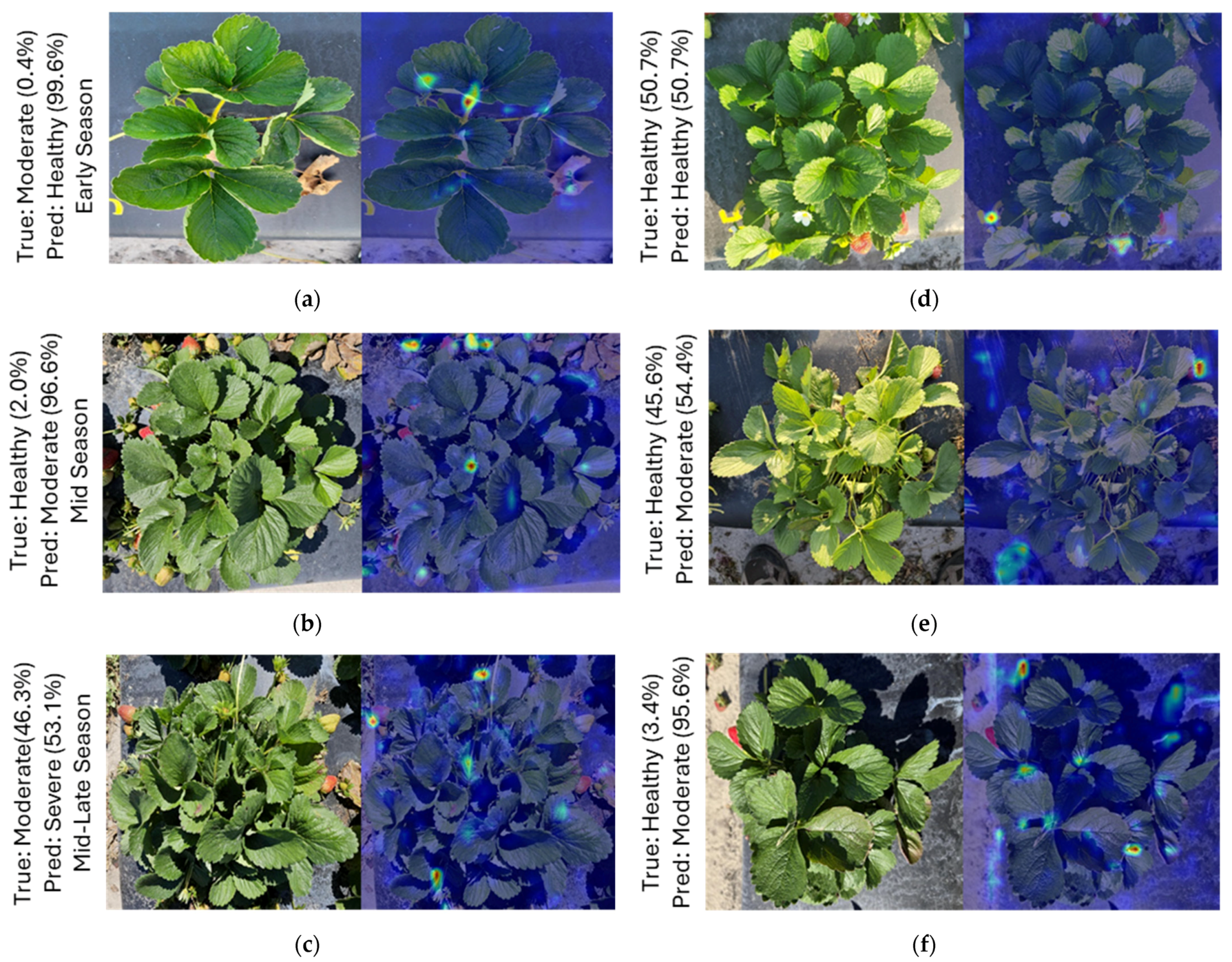
Figure 9 presents Grad-CAM visualizations for misclassified and low-confidence images, offering insight into how model uncertainty arises from both biological and dataset-level factors. Several consistent patterns were identified. First, the model is possibly associating plant size and canopy architecture with the severity stage, rather than relying on visual damage. Early-season plants with small, open canopies and visible stems were often classified as healthy even when feeding symptoms were present (Figure 9a). This bias likely stems from the training dataset, in which smaller plants were predominantly labeled as healthy. Concurrently, larger canopy plants with fruits showing signs of thrips feeding were likely to be classified as moderate (Figure 9b). Lastly, late-season plants with dense canopies and partially senescent leaves with signs of curling and plant senescence were likely to be classified as severe stage plants, regardless of actual thrips damage (Figure 8c and Figure 9c). These results indicate that the CNN learned contextual associations between growth stage and severity, correlations that are visually consistent but not biologically causal.

Second, Grad-CAM revealed attention on non-biological artifacts, such as mulch seams, bed edges, plant tags, and shadow boundaries (Figure 9d–f). These regions, which occasionally exhibited strong gradient activations, suggest that the model partially relied on background context when canopy features were ambiguous. Such artifacts likely arose from uneven lighting or spatial composition across severity classes, for instance, older plots showing more visible debris and shading, introducing unintended contextual bias.

Third, overlapping symptoms across consecutive severity stages contributed to ambiguous or split-confidence predictions; plants on the boundary between early-mid season (Figure 8a,b) and mid-late season (Figure 8c and Figure 9c) tend to have lower confidence scores. Mid-season plants often exhibited both curling and bronzing, typical of moderate damage, together with localized necrosis characteristic of severe cases (Figure 9c). In these instances, the network’s prediction confidences split almost equally for both moderate and severe stages, reflecting biological ambiguity rather than a modeling flaw. The highlighted regions in such cases covered multiple symptomatic regions, indicating that the CNN recognized features of both stages but lacked sufficient discriminatory evidence to select a single label with high certainty.

3.4.3. Implications for Symptom Recognition and Severity Staging

At infestation initiation, chilli thrips aggregate on young leaves. As infestation severity rises, chilli thrips populations spread to the entire plant, exhibiting severe symptoms on other parts of the plants [3]. However, the youngest leaves exhibited the most symptoms and were used as the labeling criteria (Table 1). The spatially relevant regions highlighted by Grad-CAM support this criterion, given the progression of pest symptomatic regions. Initially, model attention is focused on the trifoliate intersections and stems of young plants, aggregation zones of chilli thrips pests. As the plant grows older and feeding intensifies, the youngest leaves become hidden, and the symptoms begin to show on the rest of the plant, including the fruits, leaf edges, and overall canopy. These regions showed high spatial relevance in the Grad-CAM heatmaps. Plant health scouts rely on the entire plant as a whole and not just the youngest trifoliates when making diagnoses. In fact, many studies utilize fruit symptoms, flower counts, and severity of leaf curling in categorizing chilli thrips damage into different infestation stages [33,46,47]. The spatial regions the model uses in making decisions are highly relevant. These findings also reveal the need for a more holistic ground truth severity estimation framework and data annotation that considers not just the young hidden leaves, but also the older leaves, fruits, overall canopy, and other plant parts that exhibit varying symptoms. A combination of these factors can be used in developing damage thresholds for healthy, moderate, and severe stages. This will increase the complexity of the experiment, but provide the benefit of improved model robustness with an objective measure of pest severity. In addition, images of small early-season young plants with high chilli thrips infestation and large late-season healthy plants should be added to the dataset to prevent the model from learning any biases related to plant growth stage and size.

Since attaining non-intrusive images of the young hidden trifoliates is impractical in a real-time system, future applications will need to rely on canopy-level images such as the ones used in this study. This study demonstrated that top-view canopy images can be used in a real-time system for severity estimation. However, the reliability of the predictions should be improved by supplementing the dataset with more images across all growth stages and severity stages of the plant life. Additionally, to ensure minimal interference from non-biological artifacts such as shadows in a real-time system with multiple components, supplemental lighting that minimizes shadows, and image processing to remove external backgrounds can be implemented. The Grad-CAM interpretations highlight that developing accurate and reliable pest symptom classification models that can be implemented for rapid automated pest symptom detection is feasible with resource-constrained devices. This can enable the development of automated pest population control methods.

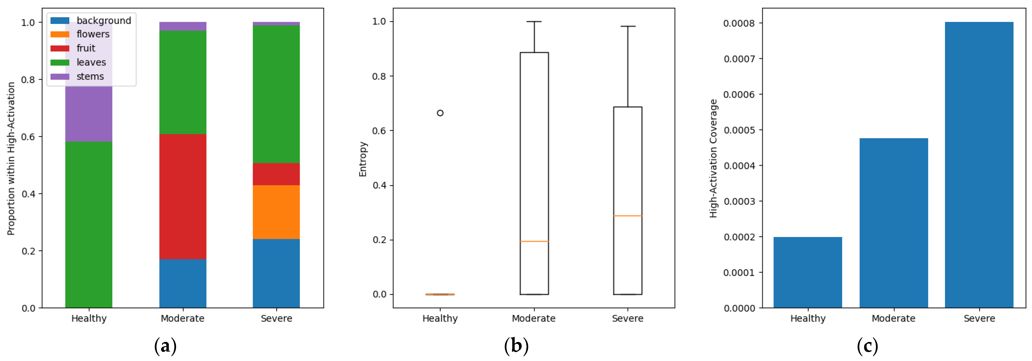
3.4.4. Quantitative Analysis of Grad-CAM Attention Patterns

Grad-CAM attention patterns were quantitatively analyzed to evaluate their consistency, spatial focus, and progression across severity stages. Figure 10 and

Table 8. Quantitative Grad-CAM Attention Statistics across Severity Stages. Values represent mean proportions of high-activation pixels (threshold ≥ 0.8) within anatomical regions, computed from ten representative high-confidence images per severity stage. Entropy quantifies attention dispersion, with lower values indicating localized activation and higher values indicating diffuse patterns.

	Background	Flowers	Fruit	Leaves	Stems	Entropy (Mean ± SD)
Healthy	0	0	0	0.583	0.417	0.066 ± 0.21
Moderate	0.170	0	0.438	0.362	0.031	0.414 ± 0.47
Severe	0.241	0.189	0.076	0.483	0.012	0.376 ± 0.41

summarize region-level attention statistics, attention dispersion, and spatial coverage for healthy, moderate, and severe classes.

Across all severity stages, Grad-CAM activations were predominantly concentrated on plant tissue rather than background regions, indicating that model predictions were primarily driven by biologically relevant visual cues. However, the spatial distribution of attention varied systematically with infestation severity. Healthy stage images exhibited highly constrained attention patterns, with activation exclusively confined to vegetative structures. On average, 58.3% of high-activation pixels were located on leaves and 41.7% on stems. This narrow spatial focus quantitatively supports visual observations that intact canopy structure characterizes healthy plants and that the model relies on stable vegetative cues when identifying the absence of infestation.

In contrast, moderate stage images showed a pronounced redistribution of attention toward reproductive and symptomatic tissues. High-activation pixels were primarily associated with fruits (43.8%) and leaves (36.2%), with a smaller contribution from background-adjacent regions (17.0%). This shift reflects the emergence of localized feeding damage during intermediate infestation stages, where discriminative cues are distributed across multiple anatomical regions rather than confined to a single structure.

Severe stage images maintained a broad attention distribution across leaves (48.3%), background-adjacent regions (24.1%), flowers (18.9%), and fruits (7.6%). Importantly, the increased overlap with background regions at this stage should not be interpreted as explicit attention to non-biological artifacts. Instead, it reflects increasingly diffuse activation patterns that extend beyond well-defined plant boundaries as canopy structure deteriorates and visually salient cues become spatially widespread.

Attention dispersion, quantified using Shannon entropy (Figure 10b, Table 8), further characterized this progression. Healthy stage images exhibited near-zero entropy values (0.066 ± 0.21), indicating highly localized and consistent attention patterns. Entropy increased substantially in moderate stage images (0.414 ± 0.47), reflecting a transition toward spatially distributed attention as multiple symptom cues emerge. Severe stage images retained elevated entropy values (0.376 ± 0.41), consistent with diffuse, canopy-wide activation patterns. Although the mean entropy was slightly higher for the moderate stage, boxplot analysis revealed a higher median entropy for the severe stage. This discrepancy reflects differences in distribution shape rather than conflicting trends. Moderate stage samples exhibited highly variable and polarized entropy values, indicative of a transitional stage with mixed localized and global attention patterns. In contrast, severe stage samples showed more consistently diffuse attention, resulting in a higher median entropy but reduced variability.

In addition to entropy, high-activation spatial coverage increased monotonically with severity stage (Figure 10c), indicating that advanced infestations produce spatially extensive visual cues that activate large portions of the canopy. These results show that model attention evolves from localized, structure-specific regions in healthy plants to diffuse, canopy-wide patterns as infestation severity increases.

3.5. Study Limitations

3.5.1. Dataset Considerations

Developing a robust chilli thrips severity classification model using full canopy RGB plant images in a complex and dynamic environment posed a few challenges, primarily associated with dataset size, temporal variability, and subjective labeling. Deep learning models typically require thousands of images to achieve stable generalization across diverse environmental conditions. The trained models in this study used 770 images (2310 with augmentations) for training, 580 for validation, and 1003 for testing. While the models achieved accuracies near 85%, the limited dataset size and class imbalance restricted further improvement. Additional imbalance mitigation strategies such as under-sampling/over-sampling the majority/minority classes, synthetic image generation, and implementing focal loss can be conducted in the future to improve model accuracy scores.

In addition, this study used a three-class mapping strategy to align with the IPM decision workflow. Stages 2–3 were intentionally merged because they fall within the same operational “action window” for biological control decisions, whereas stage 4 represents a late/intervention-failure condition. As a result, merging stages 2 and 3 into a single “moderate/action-threshold” class may reduce sensitivity to subtle physiological differences between these two stages. Particularly, early transitional cues that distinguish stage 2 from stage 3 can be partially diluted, meaning the model is optimized to detect entry into the intervention window rather than to resolve within-window progression. This trade-off is acceptable for intervention triggering but should be considered when interpreting “moderate” predictions as a coarse severity category.

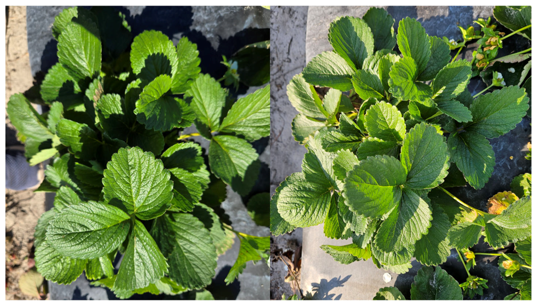
Also, environmental conditions can cause pest symptoms on the new trifoliates to intensify or reduce rapidly. An image taken of a growing plant categorized as moderate severity could change to healthy severity within a week since newer trifoliates used for ground truth data collection showed fewer signs of necrosis. However, on the canopy surface level, the plant features may not have changed considerably. Because pest severity progresses over time, images collected from the same plots may include repeated views of the same plants across different weeks and severity stages. This introduces temporal correlation between samples and may allow the model to partially rely on co-varying cues (e.g., canopy maturity, plant size, background context) that track season progression in addition to true symptom features. Figure 11 shows an example of a plant with images taken 1 week apart. The left image was labeled as a moderate stage plant, and the right image was labeled as a healthy plant. However, both images appear very similar. Such temporal instability introduces inconsistency in ground truth labeling, making symptom progression difficult to model accurately. For future experiments, improved generalization can be obtained by implementing a plant-level split that ensures that strawberry plants used in training the models are separate for validation and testing sets. Further generalization improvement strategies are discussed in the future research section.

In addition, although all data were collected at a single experimental farm, the site closely simulated commercial-farm conditions, with images captured at different times of day under varied illumination, canopy geometry, and shadow patterns. These factors introduced natural visual diversity representative of real field operations, partially addressing cross-environment variability within the same site. Explicit cross-device or multi-site validation was beyond the scope of the current study. The primary goal was to demonstrate the feasibility of real-time canopy-level severity prediction under practical field conditions rather than to perform exhaustive domain-transfer testing. The experimental setup, including on-device inference on the Jetson Orin Nano, confirmed that accurate, real-time thrips damage estimation is operationally achievable. Pest severity classification involves categorizing continuous symptoms on a discrete scale. This discretization, coupled with the subjective nature of the ground truth data collection, amplified ambiguity near class boundaries and contributed to lower top-1 accuracies of the developed models. Repeated severity assessments by multiple expert scouts using a standardized rating scheme that takes advantage of other potential symptoms of chilli thrips infestation, such as leaf curling [46,47], fruits [33], and older leaves, beyond the youngest trifoliates will improve the validity of the ground truth data and the performance of the trained models.

3.5.2. Grad-CAM Limitations

While Grad-CAM provided valuable insight into the spatial focus of model predictions, several limitations should be acknowledged. First, irrelevant background artifacts such as worker shoes, plant labels, and fruit from other plants (Figure 9d–f) occasionally influenced model activations, suggesting the need for stricter imaging protocols or automated background masking. These spurious activations may have introduced bias into learned representations, particularly in models trained on smaller datasets.

Second, this study utilized the final convolutional layer for Grad-CAM visualization because deeper layer representations effectively balance spatial information with high-level visual semantics. For most of the images analyzed, the chosen layer provided interpretable heatmaps. However, it may overlook lower-level structural cues (e.g., fine vein coloration or leaf surface texture) that may be captured in earlier layers that might be relevant in evaluating model predictions.

Lastly, Grad-CAM is a coarse localization technique that upsamples a small spatial relevance map to fit a high-resolution input image. As a result, the method cannot fully capture fine-grained symptom details that may assist in understanding model predictions. Some methods, such as Guided Grad-CAM [40], combine guided backpropagation with Grad-CAM to generate more spatially relevant heatmaps. Other XAI techniques such as LIME, LRP, etc., can also be implemented to obtain model insights. However, every method has its downsides as discussed by Kindermans et al. [48] and Adebayo et al. [49,50]. Future interpretations should consider an aggregation of multiple XAI techniques for model interpretation [30].

3.6. Future Research

As discussed in Section 3.4.2, Grad-CAM analysis revealed that the model occasionally relied on contextual cues related to plant growth stage and showed incidental attention to non-biological background artifacts. To explicitly address these limitations, future work will adopt three targeted mitigation strategies. First, the dataset will be restructured to reduce growth-stage bias by enforcing plant-level separation across training, validation, and test splits and by intentionally collecting images of small, early-season plants with confirmed moderate-to-severe infestation, as well as large, late-season plants with minimal damage. This stratified sampling will decouple infestation severity from plant maturity and canopy size. Second, data acquisition protocols will be refined to minimize background-driven attention by standardizing imaging conditions, including the exclusion of extraneous objects during image capture. In parallel, automated background masking will be explored to restrict model input to biologically relevant regions. Third, targeted model refinement strategies will be investigated, including attention-regularization techniques, to encourage the network to prioritize symptom-related plant structures.

The trained models will be implemented on the edge device connected to a controller for automated detection of pest symptoms and a variable rate release of predators for biological control of the chilli thrips pest. Subsequent work will expand validation efforts across multiple devices and geographic locations to further evaluate robustness under diverse environmental and sensor conditions. Incorporating multispectral imaging alongside canopy-level RGB imagery may also enhance early-infestation detection and cross-seasonal generalization by reducing reliance on contextual background cues.

While the present quantitative Grad-CAM analysis focused on high-confidence predictions using 10 representative images per severity class, large-scale and confidence-stratified quantitative comparisons were beyond the scope of this study. Attention patterns associated with low-confidence predictions and misclassifications were examined qualitatively; however, extending the proposed region- and entropy-based framework to explicitly incorporate prediction confidence represents an important direction for future research. Increasing the sample size of the representative images used for this quantitative analysis will enable higher accuracy estimation of population parameters, ensuring increased statistical significance for the metrics used in this study. Such extensions would enable systematic investigation of uncertainty-driven attention behavior and further strengthen the interpretability and robustness of canopy-level severity estimation models.

4. Conclusions

This study demonstrated the feasibility of real-time, canopy-level chilli thrips severity classification in strawberry production systems using deep learning and RGB imagery. By systematically evaluating multiple convolutional neural network (CNN) architectures across image resolutions, the study established that high classification accuracy (84.8%) can be achieved without reliance on close-up inspection of hidden trifoliates, which is impractical in automated field systems.

Key contributions of this work are threefold. First, the study provides a comprehensive comparative evaluation of modern lightweight and high-capacity CNN architectures under a unified data split and evaluation protocol, revealing clear trade-offs between accuracy and inference speed. While the YOLO11m-cls model with 1024-pixel input achieved the highest accuracy and macro-average recall, smaller architectures such as YOLO11s-cls, EfficientNetV2B0, and MobileNetV3Large achieved competitive performance with substantially lower computational costs, making them more suitable for deployment on resource-constrained edge devices. Second, the study introduces operationally relevant evaluation metrics, including stage-wise recall and false positive rates for the healthy class, directly linking model performance to pest management risk. This framing emphasizes that avoiding false negatives for moderate infestations is more critical than maximizing overall accuracy in integrated pest management (IPM) contexts. Third, through qualitative and quantitative Grad-CAM analysis, the study provides biological interpretability of model decisions, showing that model attention evolves systematically from localized vegetative regions in healthy plants to diffuse, canopy-wide regions as infestation severity increases.

From an actionable perspective, the results demonstrate that canopy-level RGB imaging combined with lightweight CNN models can support closed-loop pest management systems, such as automated predatory mite release platforms. The identification of fruits, leaf edges, and stems as informative visual cues suggests that future severity-rating frameworks should move beyond exclusive reliance on young trifoliates and instead incorporate whole-canopy symptom expression for more robust decision-making.

Several limitations of the present study should be acknowledged. The dataset size and class imbalance constrained further accuracy improvements, and temporal progression of the same plants introduced ambiguity near class boundaries. In addition, Grad-CAM analysis revealed that the model occasionally relied on contextual cues related to plant growth stage and exhibited incidental attention to background artifacts under ambiguous conditions. These limitations highlight the need for plant-level data separation, growth-stage–balanced sampling, and improved background control in future datasets.