Performance Prediction of Condensation Dehumidification System Utilizing Natural Cold Resources in Cold Climate Regions Using Physical-Based Model and Stacking Ensemble Learning Models

Abstract

Maintaining optimal humidity in livestock buildings during winter is a major challenge in cold climate regions due to the conflict between moisture-removing ventilation and the need for heat preservation. To address this issue, a novel condensation dehumidification system is proposed that utilizes the natural low temperature of cold winters. An integrated energy consumption model, coupling moisture and thermal balances, was developed to evaluate room temperature drop, dehumidification rate (DR), and the internal circulation coefficient of performance (IC-COP). The model was calibrated and validated with experimental data comprising over 150 operational cycles under varied operation conditions, including initial temperature differences (ranging from −20 to −5 °C), air flow rates (0.6–1.5 m/s), refrigerant flow rates (3–7 L/min), and high-humidity conditions (>90% RH). Correlation analysis showed that higher indoor humidity improved both DR and IC-COP. Four machine learning models—Extreme Gradient Boosting (XGBoost), Light Gradient Boosting Machine (LightGBM), Random Forest (RF), and Multilayer Perceptron (MLP)—were developed and compared with a stacking ensemble learning model. Results demonstrated that the stacking model achieved superior prediction accuracy, with the best R² reaching 0.908, significantly outperforming individual models. This work provides an energy-saving dehumidification solution for enclosed livestock housing and a case study on the application of machine learning for energy performance prediction and optimization in agricultural environmental control.

1. Introduction

Heating, ventilation, and air-conditioning system of micro-climate control in intensive animal house not only maintains a comfortable indoor environment, but also enhances the productivity of livestock [1,2]. However, this kind of environmental control system leads to high energy consumption, which is one of the main concerns in the breeding industry [3,4,5]. Consequently, how to effectively enhance the energy efficiency of this environmental system while maintaining animal welfare has emerged as an urgent issue in current farm management.

Especially, there is a long-term contradiction between ventilation and energy consumption in livestock and poultry production in the cold winters of Northeast China [6,7,8]. To keep an appropriate temperature for animals in winter, environment control strategies of less or non-ventilation are always used to keep warm due to the high cost of direct ventilation. However, it could result in an extremely high humid indoor environment condition, which may increase the opportunity of microorganisms’ growth and the possibility of animal respiratory diseases [9,10]. Although ventilation could decrease the humidity and exchange fresh air [11], indoor temperature can decrease rapidly at the same time. It was reported that the heat lost from livestock buildings through ventilation accounted for 70–90% of the total heat lost during winter [12]. This situation makes farmers choose between compromising animal welfare through poor air quality or high energy costs.

Currently, dehumidifiers based on the vapor-compression refrigerant cycle plays an important role in indoor moisture control. They have wide applications in residential buildings and commercial or scientific research farms [13]. To the best of the authors’ knowledge, there are few dehumidifiers used in medium- or small-scale farms in Northeast China because of the extra electricity burden [5]. As an alternative approach, condensation dehumidification (CD) is attracting increasing attention. This method leverages natural cold resources in cold climates by channeling warm, humid indoor air over a cold surface provided by the outdoor environment, causing water vapor to condense [14,15]. This process significantly reduces humidity without the heat loss associated with direct ventilation [16]. However, up to now, there are few reports on such energy-efficient dehumidification systems designed for livestock and poultry houses in cold regions [17], as well as few performance models and prediction models.

As we all know, room air temperature and relative humidity (RH) can be monitored directly by environmental sensors, but some indexes of dehumidification systems, such as dehumidification rate (DR), cooling capability (CC), and internal circulation coefficient of performance (IC-COP), cannot be monitored directly. They have to be calculated with detailed heat and mass transfer equations [18,19]. Recently, many models about moisture or heat balance for estimating the dehumidification requirement in greenhouse [18,20] and livestock house [21] have been reported. For instance, one study developed a moisture balance model to predict greenhouse air water vapor partial pressure (WVPP), and then a humidification and dehumidification demand model was developed taking into account the effective moisture capacity of the room [22]. Another model estimated humidification and dehumidification demands by considering the effective moisture capacity of the room, which can be derived from the energy balance of the enclosed space [23]. However, developing a detailed physics-based model requires many specific inputs, many of which are challenging to obtain in practice (

Table 1. Some key studies on dehumidification performance prediction in agricultural environments.

Study	Focus Area	Methodology	Key Findings	Limitations/Gaps
Rahman et al. (2021) [18].	Greenhouse dehumidification	Physics-based moisture balance model	Developed dehumidification demand model	Relies on a simplified single-equation model with empirical assumptions, omitting coupled heat–mass dynamics.
Costantino et al. (2021) [20]	Greenhouse climate control	Dynamic energy modeling	Evaluated energy performance of mechanically ventilated greenhouses	Requires numerous inputs and expert calibration; computational cost is intermediate but nontrivial.
Ding et al. (2022) [14]	Condensation dehumidification	On-site measurement + simulation	Investigated condensation dehumidification performance in humid climates	Depends on EnergyPlus simulations and is limited by model assumptions and local meteorological data accuracy.
Krommweh et al. (2014) [17]	Livestock housing with geothermal heat exchanger	Experimental and simulation study	Investigated heating/cooling potential in pig housing	Serves as a post hoc analysis tool rather than a general predictive design model.
Liu et al. (2022) [24]	Odor prediction in hen houses	Machine learning (ML) with small samples	Used ML to predict odor concentrations	Trained on small samples with limited features; ignores temporal–spatial dynamics.
Wu et al. (2021) [25]	Evapotranspiration estimation	Stacking ensemble learning	Demonstrated stacking outperforms individual models in agricultural forecasting	Purely data-driven, lacks physical basis, demands large datasets, and involves complex model tuning with high technical threshold.

). For example, parameters such as the actual thermal performance of building envelopes, latent heat release rates, infiltration rates influenced by weather and building air tightness, and the actual performance of system equipment under varying operating conditions are often difficult to measure accurately or are subject to dynamic changes. Uncertainties of these parameters in complex and variable agricultural environments can significantly affect the reliability of model predictions. Therefore, limiting the direct application of physics-based models in real-time prediction and control is very necessary [20].

Machine learning (ML) has demonstrated considerable success in predicting agricultural micro-climates, offering a powerful alternative to traditional physics-based methods [26]. ML techniques are particularly effective at modeling complex and dynamic systems. For instance, algorithms such as Extreme Gradient Boosting (XGBoost) have proven highly accurate in predicting livestock growth performance [27] and odor concentrations with small sample sizes [24]. Likewise, recurrent neural networks (RNNs) are good at capturing temporal dependencies and have been widely used in energy consumption forecasting [28,29]. While individually powerful algorithms like XGBoost and RNNs can be further enhanced through stacking integration. This ensemble approach builds a unified framework that achieves greater predictive accuracy and robustness, as demonstrated in various agricultural forecasting tasks. For example, an ensemble learning framework based on Support Vector Machine (SVM) and Relevance Vector Machine (RVM) was developed to address the challenges of low accuracy and poor interpretability in small-sample and nonlinear scenarios in accurate biogas prediction [30]. Similarly, a stacking framework effectively integrated multi-angle spectral and texture features from canola growth UAV imagery to precisely estimate key parameters like leaf chlorophyll content [31]. Furthermore, for daily precise reference evapotranspiration estimation across different climate regions, stacking models consistently outperformed both basic machine learning models and empirical approaches while showing excellent portability [25] (Table 1). These implementations demonstrate the model’s capacity to effectively integrate heterogeneous models and data sources, thereby offering reliable support for precision agriculture.

So, according to analysis the dehumidification status of livestock house and prediction algorithms, the research gaps, and challenges are concluded as follows:

(1) Existing condensation dehumidification systems are mostly not tailored to the indoor high-humidity, outdoor low-temperature characteristics of livestock housing.

(2) Physics-based models require numerous precise input parameters, making them limited in applicability within complex and variable livestock environments.

(3) Although machine learning has been applied in agricultural environmental prediction, ensemble learning frameworks have not yet been employed for multi-indicator cooperative prediction and energy efficiency optimization of condensation dehumidification systems in livestock housing.

Therefore, the condensation dehumidification system presented in this study was designed to address the specific environmental control challenges in enclosed livestock housing during cold winters, namely the conflict between moisture removal and heat preservation. The core design philosophy prioritizes maximizing the utilization of natural cold resources while minimizing active energy consumption and indoor heat loss. The detailed research aims are as follows:

(1) Design a novel condensation dehumidification system suitable for livestock housing in cold regions, fully utilizing natural cold sources in winter to achieve low energy costs;

(2) Develop a coupled moisture and thermal balance model to generate system performance datasets that align with the practical conditions of livestock environment;

(3) Propose and apply a stacking ensemble learning framework to achieve high-accuracy prediction of key system performance indicators (room temperature drop (TD), DR, and IC-COP), providing decision support for intelligent control and optimized operation of the system.

This study not only provides a feasible energy-saving dehumidification solution for livestock housing in cold regions but also offers a methodological reference for the intelligent prediction and optimization of agricultural environmental control systems.

The paper is organized as follows. Section 2 describes the system design, the physics-based model, and the machine learning framework. Section 3 presents the data analysis and model performance comparison. Section 4 discusses the advantages and limitations of the ensemble learning approach, and Section 5 summarizes the key findings and implications and prospective future directions.

2. Materials and Methods

2.1. Design of Dehumidification Process

The design of this dehumidification system aims to resolve the conflict between moisture removal and heat preservation for humidity control in livestock houses during cold winters. The system utilizes the natural low temperature of winter as a cold source, achieving cold energy storage through the outdoor heat exchanger and the insulated tank, thereby avoiding the heat loss associated with conventional ventilation methods. During the indoor dehumidification phase, the chilled refrigerant flows through the indoor heat exchanger, causing the warm and humid room air to condense and remove moisture. With its simple structure, the system is suitable for enclosed livestock environments and provides a feasible energy-saving solution for humidity control in livestock housing under cold climatic conditions.

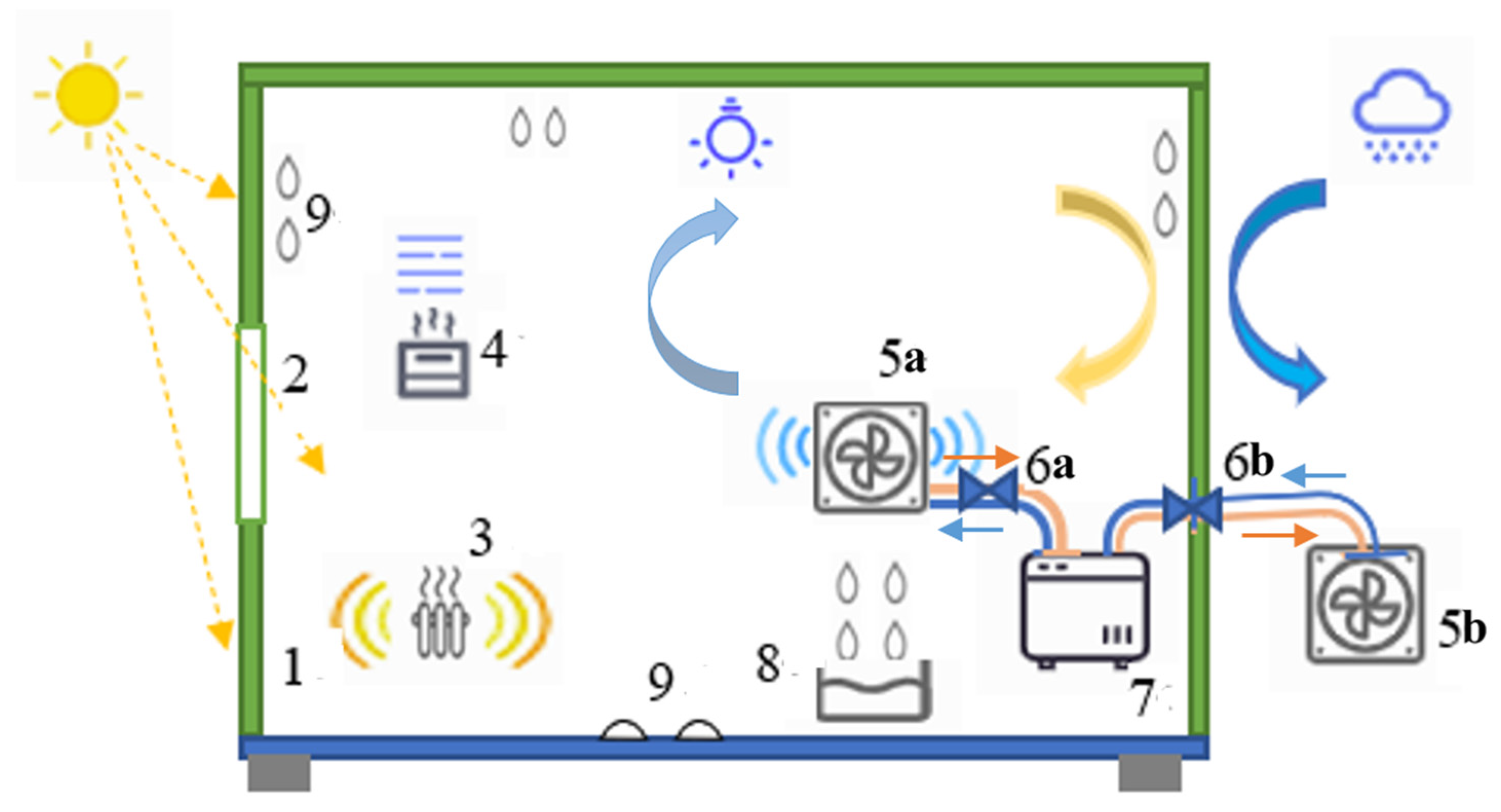
This dehumidification system designed mainly consists of indoor and outdoor heat exchangers equipped with fans, an insulation tank, two refrigerant circulating pumps and connecting pipes within an enclosed chamber (Figure 1). To simulate the high-humidity environment, a steam generator is used as the moisture source in this enclosed chamber, while a heater provides primary warming to the indoor space. Water sink is used for condensate water collection. Indoor and outdoor fans are useful to accelerate energy transfer.

When outdoor ambient temperature is low, especially at night, circulating pump 6b works. Refrigerant is delivered to outdoor heat exchanger 5b to release heat. The chilled refrigerant then returns into the tank and preserves cool energy.

When dehumidification is required, refrigerant circulating pump 6a works. Chilled refrigerant passing into the tubes of indoor heat exchanger 5a makes a local low temperature. Warm and humid room air is imported by indoor fan equipped on heat exchanger 5a. Low-temperature heat exchanger makes this air temperature drop below the dew point of the saturated humidity and precipitates condensate water. If the outdoor ambient temperature is relatively low, the outdoor circulating Pump 6b could be turned on during the whole process of dehumidification.

During the process of dehumidification, the refrigerant in the system is slowly heated up. When the room’s relative humidity has dropped to the target level or the unit can no longer effectively condense water, the condensation system stops.

2.2. Experimental Materials and Properties

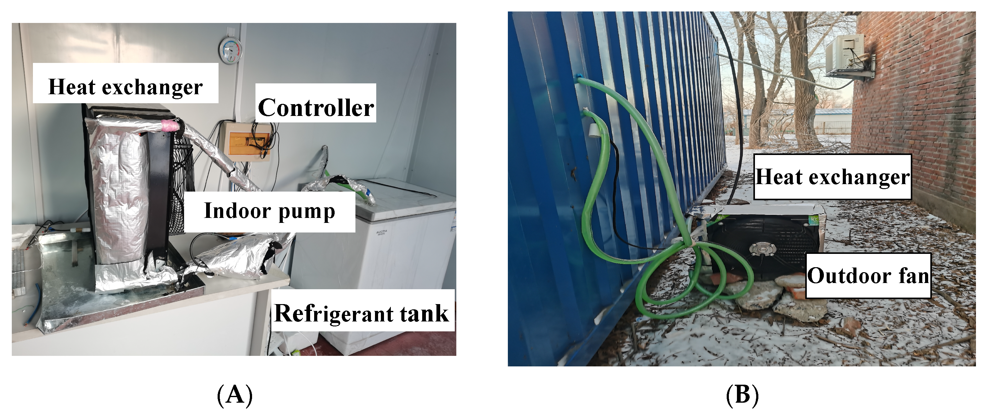
To evaluate the main impact factors (TD, DR, and IC-COP) of this humidification system, a series of experiments were carried out in the laboratory of Northeast Agricultural University, Harbin, Northeast China from November to February 2022 and 2023. Harbin is located between 125°41′ to 130°13′ N and 44°04′ to 46°04′ E. The average outdoor temperature in January was about −19 °C, and RH was about 72%. An enclosed chamber was placed outdoor. The walls and ceiling of the chamber were made of 5 cm rock wool sandwich panels, and the floor was made of 1.5 cm Magnesium Oxide board. Rated power of the fan and refrigerant pump were 190 W and 46 W, respectively. In total, 70 L refrigerant was stored in a 202 L insulation tank in the chamber (Figure 2). The core function of this tank is to store the refrigerant and utilize the insulation to reduce cold energy loss, thereby maintaining the initial refrigerant temperature. Refrigerant is an ethylene glycol aqueous solution, with a freezing point below −45 °C and a specific heat capacity of approximately 3.35 kJ/(kg·K).

Table 2. Primary parameters of experiment objects.

Chamber	Parameters
Length × width × height of chamber	5.80 m × 3.00 m × 2.40 m
Length × width of window	1.17 m × 1.02 m
window orientation	West
Heat exchanger	Parameters
Length × width × height of indoor heat exchanger	0.53 m × 0.18 m × 0.53 m
Length × width × height of outdoor heat exchanger	0.38 m × 0.18 m × 0.38 m
Total heat exchange area of indoor heat exchanger	18 m2
Total heat exchanger area of outdoor heat exchanger	10 m2
Average pin thickness	0.33 mm
Pin channel gap	3.02 mm
Diameter of tube	0.89 cm

showed primary parameters of experiment conditions.

Wet-bulb and dry-bulb temperature sensors and anemometers were located on inlet and outlet of the heat exchanger, and temperature and humidity sensors and static pressure sensors were installed to monitor the ambient situation change (

Table 3. Characteristics of the measurement devices.

Device	Type	Range	Accuracy	Note (Manufacturer; Model)
Wet-bulb temperature	Thermocouple	0 to 80 °C	±1.0 °C	CEM, Shenzhen, China; DT-8896
Air flow rate	Differential pressure sensor	0.3–45 m s−1	0.1 m/s	Smart Sensor, Dongwan, China; AS836
Static pressure	Differential pressure sensor	0–1000 Pa	±0.3%	Bendu, Shanghai China; YE-100
Temperature	Thermocouple	−40 to 80 °C	±0.1 °C	Shandong Jingxun, Weihai, China; JXBS-3001-TH
RH	Thermocouple	0–100%	±1%	Shandong Jingxun; Weihai, China; JXBS-3001-TH

). The measuring equipment used in this study was calibrated before the experiment to ensure their respective rated accuracy. Control system collected data on indoor and outdoor temperature and humidity to control the operation on fans and refrigerant pumps.

2.3. Experimental Parameter Setting

This experiment systematically evaluates the performance of the dehumidification system under simulated conditions of indoor high humidity and outdoor low temperature typical of winter. The experimental design is a multi-factor test, with key control parameters including the initial temperature difference between indoor air and refrigerant (Init. TDiff), fan air flow rate (AFR), refrigerant flow rate (RFR), and heater power. The rationale for selecting these parameters is as follows: the initial indoor air temperature range (15–20 °C) is set according to suitable winter temperatures in livestock house; the initial refrigerant temperature gradient (−20 °C to −5 °C in 5 °C increments) is used to investigate dehumidification effectiveness; and the ranges for AFR and RFR are determined based on indoor air velocity limits (≤2.0 m s⁻¹) in livestock houses and typical system operating conditions as detailed in

Table 4. Experimental scheme design of CD.

No	Outdoor T, °C	Initial Room T, °C	Initial Refrigerant T, °C	AFR, m s−1	RFR, L min−1	Heater Power, kw h−1
1	−22~−7.9	15/20	−5/−10/−15	0.6/0.9/1.5	3/5/7	5.537
2	−24~−7.0	20	−5/−10/−15/−20	0.6/0.9/1.5	3/5/7	4.400

. To simulate high-humidity conditions, the initial relative humidity in the test chamber was controlled above 90%. The experiments comprise over 150 operational cycles. This design was chosen over alternatives primarily for its potential for high energy efficiency (IC-COP) in high-humidity, low-ambient-temperature conditions, aligning with the climatic context of Northeast China’s winters.

The data collection procedure was as follows: After system startup, both indoor and outdoor fans and the refrigerant circulation pump were activated simultaneously. The air temperature and humidity at the inlet and outlet of the heat exchanger were continuously monitored until the temperature (T) and RH inside the enclosed indoor chamber reached steady state (defined as a change rate of less than ±3% per unit time). Steady-state data were recorded and used for subsequent analysis and modeling.

Regarding subsequent modeling and validation, a stratified random split was applied during machine learning modeling to divide the data into training (80%) and test (20%) sets, ensuring the model’s generalizability to unseen data. Hyperparameter tuning was performed using grid search combined with cross-validation. The final model performance was evaluated on an independent test set. Relevant results and discussions are presented in Section 4 of this paper.

2.4. Theories of Moisture and Thermal Balance Model

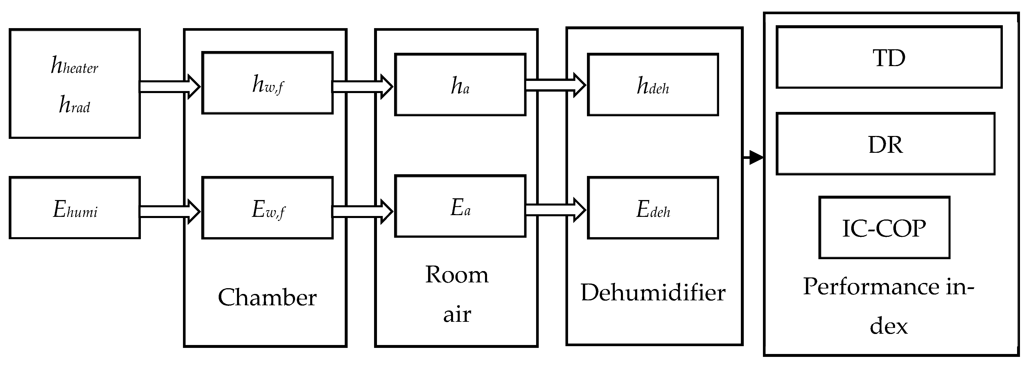
The analysis process of the indoor moisture and heat composition is as follows (Figure 3):

For moisture control, a steam generator is used as the main moisture source. Without ventilation, condensation of the inner surface of chamber and dehumidifier designed are two main moisture sinks in this experiment. The exothermic condensation process occurs all the time on the inner cover surface because of much lower outdoor ambient temperature than indoor in winter. The amount of this condensate generated in winter is too significant to be ignored. On the other hand, room air plays a key role as a moisture adjuster. It is a moisture sink when the produce speed of water vapor is greater than the reduction speed of water vapor before air saturation; otherwise, it is a moisture source when the temperature of room air is lower than the dew point temperature at that air pressure, which leads to air condensation in this condition.

For thermal control, the main heat source in this enclosed chamber is an electric heater. The solar radiation is a small heat source through the window during the daytime. Because of init. TDiff between outdoor and indoor, a great amount of indoor heat is dissipated out from the wall and floor of the chamber. Dehumidifier based on condensation will also decrease the indoor temperature by chilled refrigerant, which consumes a large amount of heat energy in this system.

2.4.1. Thermal Balance Model Establishment

(1) Electric heater

The heat output from the electric heater ($h_{heater}$) was calculated using the following equation:

$$h_{heater}=\eta H_{heater}$$

(1)

where $h_{heater}$ is the effective output power, W; $H_{heater}$ is the rated input power, W; and $\eta$ is the efficiency of the heater (dimensionless) [32].

(2) Solar radiation heat module

This module estimates the heat produced by the solar radiation, which enters through the window. The heat of solar radiation has a small influence both because of the small size of the window and low radiation intensity in winter in cold climate regions. The heat power of solar through the window is calculated as Equation (2),

$$h_{rad}=0.889\times I\times c\times A_{win}$$

(2)

where h_rad is solar power through the window, W; I is solar radiation intensity, W m⁻²; c is integrated shading coefficient of external window, dimensionless; A_win represents the area of window, m²; and 0.889 is the standard reference value for the total solar energy transmittance [33].

(3) Heat released from wall and floor

Indoor heat is dissipated out from the walls and the floor. The releasing of heat energy can be calculated by Equation (3),

$$h_{w,f,win}=q\times (T_i-T_o)\times A$$

(3)

where h_w,f,win is heat released by wall, floor, and window, W; T_i, T_o represents the indoor and outdoor temperature, respectively, °C; and A represents the total area of wall, floor, and window, respectively, m² [32].

(4) The energy absorbed or released due to the temperature change in air can be calculated using Equation (4),

$$h_a=C_a\times \rho \times V\times \Delta T/3600$$

(4)

where h_a is the absorption and release energy from the air, W; C_a is air specific heat capacity, J kg⁻¹ K⁻¹; ρ is air density, kg m⁻³; V is chamber volume, m³; and ΔT is temperature difference, °C [32].

(5) Dehumidifier

The process of dehumidification based on CD is exothermic. Based on the above conditions, the CC of the dehumidifier was expressed as Equation (5),

$$h_{deh}=h_{heater}+h_{rad}-h_{w,f,win}-h_a$$

(5)

where h_deh is the cool capability of the dehumidifier, W.

Equation (5) provides a simplified expression for the cooling capacity, derived from sensible heat exchange between air and refrigerant. It does not explicitly account for heat losses from heat exchangers, pipelines, and the storage tank, or for parasitic heat gains from fans and pumps. These simplifications are justified given the well-insulated experimental setup and the relatively low power of auxiliary devices (fan: 190 W, pump: 46 W).

2.4.2. Moisture Balance Model Establishment

(1) Steam generators

The main moisture source in enclosed chamber is steaming generators, which produces a certain amount of moisture into the indoor air. E_humi represents the amount of moisture production.

(2) Condensation of cover inner wall and floor

The condensation rate is proportional to the difference between the water vapor partial pressure (WVPP) of the indoor air and the saturation WVPP at the cover inner surface temperature. It can be calculated as Equation (6) [34],

$$E_{w,f}=3600\times {\displaystyle \frac{0.67\times q\times (e_i-e_{sc})}{C_a\times P}}$$

(6)

where E_w,f is condensation water rate, in kg h⁻¹ m⁻²; q is convective heat transfer coefficient at the cover inner surface of wall or floor, in w m⁻² k⁻¹; e_i is the water vapor pressure of the indoor air, kPa; and e_sc is the saturation air water vapor pressure the inner cover surface temperature, kPa.

(3) Moisture changes in room air

In this module, the room air water content is studied by using the theory of wet air. To simplify the calculation, the following assumptions are made: (1) wet air has a constant physical property, which is composed of dry air and water vapor; (2) the contact thermal resistance of fin-tube is ignored, and the influence of environmental thermal radiation is ignored; (3) the fouling factor is ignored. It was expressed as Equations (7)–(9),

$$W=0.622{\displaystyle \frac{\varphi P_s}{100P-\varphi P_s}}$$

(7)

$$m_{vapor}=m_{dry}W$$

(8)

$$E_a=\Delta m_{vapor}/\Delta t$$

(9)

where W is moisture content, kg·kg⁻¹ (dry air); Φ is room air RH, %; P_s is the partial saturation vapor pressure, kPa; P is atmosphere pressure, kPa [32]; m_dry is dry air mass in enclosed chamber, kg; m_vapor is water vapor mass in air, kg; Δm_vapor is water vapor mass difference between two time points, kg; Δt is time difference, min; and E_a is DR, kg h⁻¹. The physical properties of room air are obtained in saturation vapor pressure table and air density table [35].

The temperature and RH in the test chamber are collected by the temperature and humidity sensors. The air moisture content is calculated using Equation (7). Combined with the air density table and the chamber volume, water vapor mass is calculated using Equation (8). The DR of water vapor in any length of time can be calculated using Equation (9).

(4) Dehumidifier

Based on the above conditions, the following model for dehumidification based on moisture balance can be developed below,

$$E_{deh}=E_{humi}-E_{w,f}-E_a$$

(10)

where E_deh is the dehumidification that is removed by dehumidification system at time t, kg h⁻¹; E_humi is the moisture added to the chamber by humidifier, in kg h⁻¹; E_w,f is the moisture removed from the air by condensation from cover inner wall and floor, kg h⁻¹; and E_a is the moisture absorbed or released from the air, kg h⁻¹.

2.5. Model Assumption and Limitation

To establish the physical-based model of moisture and thermal balance, the following key assumptions were made with certain associated limitations [20,35,36]:

(1) Uniformity assumption

The air temperature, humidity, and psychrometric properties within the experimental chamber are assumed to be uniformly distributed. This is a common simplification for whole-room energy and mass balance models. In this study, based on the active air mixing provided by the integrated fan on the indoor heat exchanger, the average data from multiple temperature and humidity sensors placed at different locations was used in conjunction with system-level performance prediction models [20,37].

(2) Quasi-Steady-State calculation

The model treats the chamber’s environmental parameters as constant within each calculation time step (1 min). This is suitable for relatively slow-changing processes but may not fully capture the details of intense transient fluctuations [35].

(3) Thermophysical properties

The properties of air and refrigerant (such as specific heat capacity, density) are treated as constants or as varying simply with temperature, without considering their nonlinear variations across the full range of temperature and humidity conditions [35].

(4) System boundaries

The model primarily focuses on the interaction between the chamber air and the heat exchanger/enclosure structure. Details such as pressure drops within the refrigerant circuit and variations in pump efficiency are not incorporated into the model [36].

(5) Simplifications in energy and mass balance [18,22]:

1) Cooling capacity calculation (Equation (5)): This formula is primarily based on sensible heat exchange between the air side and the refrigerant side. The model does not explicitly include heat dissipation losses from the heat exchanger, piping, and storage tank, nor does it account for the minor heat gain from the operation of fans and pumps. These omissions may lead to an overestimation of the actual cooling capacity.

2) Condensation model (Equation (6)): Surface temperature is iteratively updated using the heat balance equation from the previous time step, rather than solving dynamic partial differential equations in real time.

3) Solar radiation module (Equation (2)): A standard value for total solar energy transmittance is used, and an integrated shading coefficient is considered. However, dynamic simulation of variations in solar incidence angle and multiple reflections/absorption by indoor surfaces is not included.

These assumptions allow the model to achieve a balance between computational complexity and practicality, making it suitable for evaluating the system’s macroscopic performance and trend analysis. The calibration and validation of the model based on full-scale experimental data (Section 3.1) compensate to some extent for the errors introduced by these simplifications.

2.6. Performance Indices

The performance of the dehumidifier was evaluated using indoor TD, DR, and IC-COP as performance indicators.

(1) TD

Indoor temperature fluctuation is an important factor of environmental control in livestock house. It reflects the CC of this dehumidifier and influences the temperature compensation in future research. This factor can be obtained by multiple temperature sensors placed at different locations.

(2) DR

To evaluate the dehumidification performance of this system, DR is the primary index, which can be calculated by Equation (10).

(3) IC-COP

The IC-COP is defined as the ratio of the useful cooling capacity provided within the process air loop to the electrical power input solely for the fluid-moving auxiliary devices (fans and pumps). It explicitly excludes the energy input for regeneration heating, which is analyzed separately. Therefore, it evaluates the efficiency of the internal air and fluid-handling subsystem. IC-COP of the dehumidifier is estimated by Equation (11),

$$IC\text{-}COP={\displaystyle \frac{h_{deh}}{\sum H_{fan}+\sum H_{pump}}}$$

(11)

where h_deh is the CC of dehumidifier, W; H is the overall operating electric energy consumption of the dehumidifier, including energy consumptions of indoor and outdoor fans and pumps, W.

2.7. Prediction Algorithms

2.7.1. Basic Models

The selection of base machine learning models—XGBoost, LightGBM, Random Forest (RF), and Multilayer Perceptron (MLP)—was based on their proven effectiveness in handling complex, nonlinear relationships in agricultural environmental prediction tasks. XGBoost and LightGBM are known for their high efficiency and robustness in small-to-medium datasets, which aligns with our experimental data scale (about 150 cycles). RF was chosen for its resistance to overfitting and ability to capture feature interactions without extensive tuning. MLP was included to model potential high-order nonlinearities through its deep architecture. These models collectively provide a diverse set of inductive biases, ensuring that the ensemble can capture a wide range of patterns in the dehumidification system’s behavior [27,38].

(1) XGBoost

XGBoost, a highly efficient and scalable tree-based algorithm, operates on the principles of gradient boosting and ensemble learning [39]. It constructs multiple decision trees sequentially. Each new tree trained to correct the residuals of the combined previous models. The most important advantage is its incorporation of regularization techniques which effectively controls model complexity. The final prediction is formed by aggregating the outputs of all trees through a weighted summation. Recently, XGBoost has been widely adopted as a dominant tool for both regression and classification tasks.

(2) LightGBM

LightGBM, a high-performance gradient boosting framework [40], operates on the principles of ensemble learning with a focus on training speed and efficiency. It constructs decision trees using a novel technique that grows tree leaf-wise rather than level-wise, and leverages histogram-based algorithms to bundle sparse features. The main advantage is that these optimizations allow it to handle large-scale data with significantly lower memory usage and faster training times. The final prediction is formed by aggregating the outputs of all trees in a similar manner to other gradient boosting methods. Now, LightGBM has been widely adopted for a wide range of machine learning tasks.

(3) RF

RF, a prominent tree-based algorithm introduced by Breiman [41], operates on the principles of bagging and ensemble learning. It constructs multiple decision trees (CART models) by training each on a unique bootstrap sample from the dataset. These trees are independent and can be built in parallel. The final prediction is formed by aggregating the outputs of all trees through a ‘voting’ mechanism for classification or averaging for regression. Owing to its user-friendly nature, relatively few hyperparameters, and resistance to overfitting, RF has been widely adopted for both regression and classification tasks.

(4) MLP

MLP, or artificial neural network (ANN), comprises an input layer, at least one hidden layer, and an output layer. As a fundamental feed-forward neural network, MLP is extensively used for analyzing complex problems and serves as a base for more advanced architectures like Convolutional neural networks (CNNs) and Deep Neural Networks (DNNs) [38,42].

To systematically evaluate the sensitivity of model performance to key hyperparameters and identify the optimal configuration for our dataset, four distinct hyperparameter sets were defined for each base learner (XGBoost, LightGBM, RF, MLP). These sets are named according to their design emphasis as follows:

(1) Baseline: Configurations using the default hyperparameter values as specified in the original algorithm implementations or widely adopted standard libraries. This serves as a common reference point.

(2) Conservative: Configurations designed to prioritize generalization and prevent overfitting by reducing model complexity. This typically involves stricter regularization, shallower trees (for tree-based models), fewer neurons/layers (for MLP), and smaller learning rates.

(3) Aggressive: Configurations designed to maximize model capacity and fitting ability on the training data, accepting a higher risk of overfitting. This typically involves weaker regularization, deeper trees, more neurons/layers, and larger learning rates.

(4) Balanced: Configurations manually tuned via preliminary search to achieve a practical compromise between the conservative and aggressive extremes, often yielding robust performance without clear underfitting or overfitting.

(5) MoreLeaves: For tree-based models, this configuration increases the num_leaves parameter or similar parameters controlling the maximum number of leaf nodes in a tree. This allows the tree to create more finer-grained decision splits, increasing model complexity and capacity to fit detailed patterns in the data.

(6) Deep: For MLP, it indicates a network architecture with more hidden layers (increased depth) to enhance its ability to learn hierarchical feature representations.

(7) Wide: Primarily for MLP, this configuration increases the number of neurons per hidden layer (increased width) while potentially keeping the number of layers modest. A wider network can learn to detect more features in parallel within a layer.

2.7.2. Hyperparameter Tuning Strategy

To systematically optimize the performance of each base model, a grid search with 5-fold cross-validation was conducted on the training set. The hyperparameter search ranges and the optimal values selected for each model are summarized in

Table 5. Hyperparameter tuning configuration and optimal values for the base machine learning models.

Model	Hyperparameter	Search Range /Candidates	Description/Purpose
XGBoost	n_estimators	[100, 200, 300, 500]	Number of boosting rounds (trees).
	max_depth	[3, 5, 7, 10]	Maximum tree depth. Controls model complexity to prevent overfitting.
	learning_rate	[0.01, 0.05, 0.1, 0.2]	Step size shrinkage used in update to prevent overfitting.
	subsample	[0.6, 0.8, 1.0]	Subsample ratio of the training instances.
	colsample_bytree	[0.6, 0.8, 1.0]	Subsample ratio of columns when constructing each tree.
LightGBM	num_leaves	[15, 31, 63, 127]	Maximum number of leaves in one tree. Primary control for complexity.
	max_depth	[−1, 5, 10, 15] (where −1 means no limit)	Maximum tree depth.
	learning_rate	[0.01, 0.05, 0.1]	Boosting learning rate.
	n_estimators	[100, 200, 300]	Number of boosting iterations.
	min_child_samples	[10, 20, 30]	Minimum number of data needed in a leaf (child).
RF	n_estimators	[100, 200, 300, 500]	Number of trees in the forest.
	max_depth	[10, 15, 20, None]	Maximum depth of the tree. None means nodes are expanded until pure.
	min_samples_split	[2, 4, 6]	Minimum number of samples required to split an internal node.
	min_samples_leaf	[1, 3, 5]	Minimum number of samples required to be at a leaf node.
MLP	hidden_layer_sizes	[(64,32,16), (128,64), (100), (50,50,50)]	Number of neurons in each hidden layer.
	activation	[‘relu’, ‘tanh’, ‘logistic’]	Activation function for the hidden layers.
	solver	[‘adam’, ‘sgd’]	The solver for weight optimization.
	learning_rate_init	[0.001, 0.0005, 0.0001]	The initial learning rate used by the solver.
	max_iter	[300, 400, 500]	Maximum number of iterations.

. The tuning process aimed to maximize the R² score while preventing overfitting.

Hyperparameter optimization was performed on the training set (80% of the data) to identify the optimal combination of hyperparameters for each model, maximizing the R² score. The final models were evaluated on the held-out test set (20% of the data).

2.7.3. Stacking Ensemble Learning Models

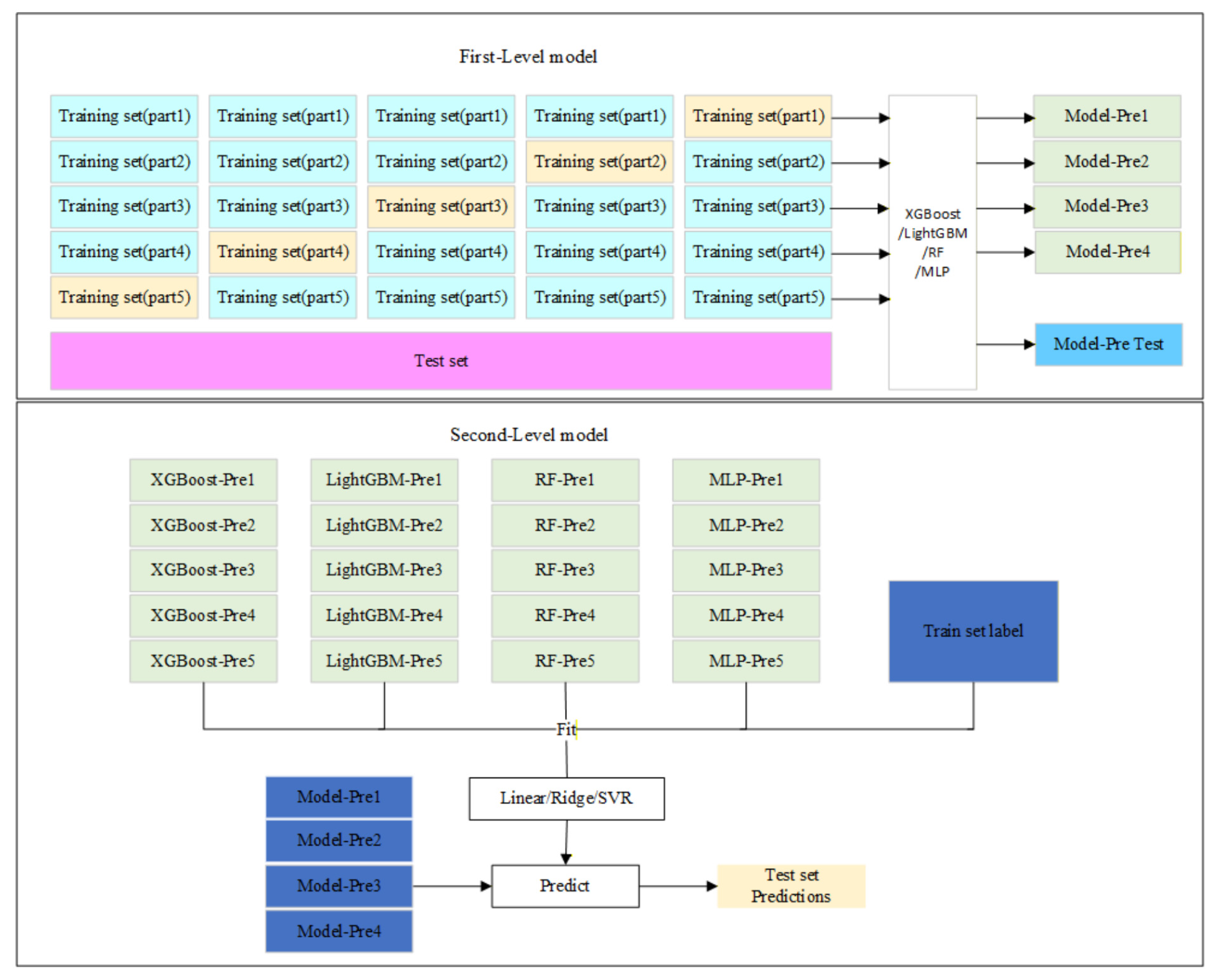
To further enhance prediction accuracy and robustness beyond the capability of any single model, a stacking ensemble framework, which is a hierarchical ensemble framework, was employed. Its core idea is to combine multiple heterogeneous base models and integrate their predictions through a meta-learner to achieve performance superior to that of any single model [43]. This approach has been successfully demonstrated to achieve superior predictive performance in complex agricultural environmental modeling tasks.

In the standard two-layer stacking structure, first level consists of multiple heterogeneous base models responsible for transforming the original data into meta-features. Second level comprises a meta-learner, which takes the meta-features output from the previous layer as input to generate the final prediction. To prevent overfitting and fully utilize all training data in generating meta-features, the K-fold cross-validation method is commonly employed during the training of the first level models (Figure 4).

2.7.4. Data Partitioning for Model Evaluation

To ensure a rigorous evaluation of model generalizability, the entire experimental dataset was randomly split into a training set and a completely independent test set, with a ratio of 80% for training and 20% for testing. The hyperparameter tuning for all base models (XGBoost, LightGBM, RF, MLP) and the training of the stacking ensemble (including the 5-fold cross-validation for meta-feature generation) were conducted exclusively on the training set. All performance metrics (R², MSE, MAE) (Section 2.8) are calculated solely based on the predictions made by the final trained models on the held-out test set.

2.8. Comparison Metrics

In this study, the coefficient of variation in coefficient of determination (R2), Mean Squared Error (MSE), and Mean Absolute Error (MAE) are selected to validate the prediction performance.

$$R^2=1-{\displaystyle \frac{{\sum }_i(y_i-{\widehat{y}}_i{)}^2}{{\sum }_i(y_i-{\widehat{y}}_i{)}^2}}$$

(12)

$$MSE={\displaystyle \frac{{\sum }_i(y_i-{\widehat{y}}_i{)}^2}{N}}$$

(13)

$$MAE={\displaystyle \frac{{\sum }_i|{\widehat{y}}_i-y_i|}{N}}$$

(14)

where n denotes sample size; y_i denotes the true/actual value of the i-th sample; and ŷ_i denotes the predicted value of the i-th sample.

3. Results

3.1. Statistics and Correlation Analysis

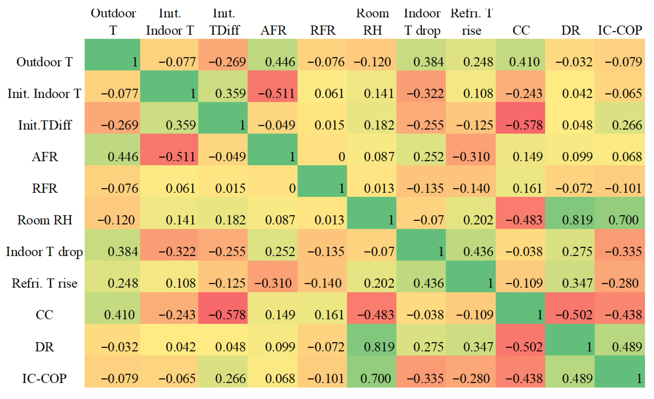
Based on the monitored and derived experimental data, correlation coefficients of the influencing factors of the dehumidification system (outdoor T, init. TDiff, AFR and RFR) and dehumidification performance factors (indoor RH, indoor T, refrigerant T rise, CC of dehumidifier, DR and IC-COP) were determined by the Spearman correlation analysis method (

Table 6. Variables of experimental performance data.

Data	Indoor T Drop, °C	Refrigerant T Rise, °C	CC, kw	DR, kg h−1	IC-COP
Min value	0.2	3.9	10.53	2.84	2.39
Max value	9.4	19.3	30.77	4.79	5.71
Average ± STD	5.03 ± 2.06	10.52 ± 3.68	20.77 ± 4.88	4.39 ± 0.28	3.91 ± 0.87

) [44]. The resulting correlations were visualized with the heatmap [45], as shown in Figure 5.

Spearman’s correlation was calculated for all variables to obtain an overview of all correlations. The correlation coefficient has a value between −1 and 1, where 1 is total positive correlation, 0 is no correlation, and −1 is total negative correlation. In the literature, it is helpful to find different interpretations and rankings of correlation coefficients in terms of statistical significance.

(1) Impact on DR

For DR, the main driving factor in the entire Spearman matrix was indoor relative humidity (0.819). This indicated that relative humidity was the main factor determining DR. The secondary influencing factor was AFR (0.099), indicating that increasing airflow slightly promotes dehumidification.

(2) Impact on system IC-COP

For IC-COP, the main driving factors were room relative humidity (0.700) and DR (0.489), which means higher dehumidification capacity and energy efficiency are achieved in high-humidity environments. Init. TDiff (0.266) also had a positive effect on improving IC-COP. In contrast, a decrease in indoor temperature (−0.335) and an increase in cooling temperature (−0.280) suppressed IC-COP, indicating that excessive temperature changes during operation can reduce energy efficiency.

(3) Impact on CC

For CC, init. TDiff (−0.578) was a key inhibitory factor, which meant larger differences can lead to lower cooling capacity, which may be due to changes in heat-exchange efficiency under high temperature differences. The outdoor temperature (0.410) had a positive impact on CC, which may be due to difficulties in outdoor heat dissipation leading to an increase in refrigerant reflux temperature and an increase in indoor sensible heat cooling. The relative humidity of the room (−0.483) suppressed CC because more energy was allocated to latent heat (dehumidification) rather than sensible heat cooling.

3.2. Model Comparison

Table 7. Comparison of individual model performance.

Model	MSE	MAE	R2	Best R2	Average R2
XGBoost_Conservative	0.018	0.107	0.737	0.765	0.732
XGBoost_Balanced	0.016	0.102	0.765
XGBoost_Aggressive	0.024	0.122	0.648
XGBoost_Baseline	0.015	0.098	0.777
LightGBM_Conservative	0.020	0.112	0.710	0.777	0.740
LightGBM_Balanced	0.017	0.104	0.748
LightGBM_MoreLeaves	0.017	0.105	0.744
LightGBM_Baseline	0.016	0.101	0.760
RF_Deep	0.018	0.106	0.721	0.759	0.710
RF_Conservative	0.012	0.109	0.688
RF_Balanced	0.017	0.102	0.736
RF_Baseline	0.019	0.109	0.697
MLP_Deep	0.020	0.115	0.695	0.784	0.728
MLP_Wide	0.018	0.108	0.719
MLP_Conservative	0.014	0.096	0.784
MLP_Baseline	0.018	0.113	0.714

showed the prediction performance of four base machine learning models under different hyperparameter configurations.

Overall, XGBoost and LightGBM demonstrated the most stable performance. XGBoost_Baseline model achieved the highest R² score of 0.777. While the MLP model performed moderately under its default configuration, its MLP_Conservative version achieved the best performance among all individual models (R² = 0.784) after optimization. The RF model’s performance was relatively weaker (R² = 0.736).

Table 8. Analysis of optimal model configurations.

Model_Name	Best_MSE	Best_R2	Layers/Depth/Nodes/Estimators	Learning_Rate	Activation_Function	Other_Params
MLP_Conservative	0.014	0.784	Number of hidden layers: 3; Network structure: (64, 32, 16)	0.0005	tanh	solver: adam, max_iter: 400
XGBoost_Baseline	0.015	0.777	Tree dept: 3; Number of trees: 300	0.01	Decision tree	colsample_bylevel: None
LightGBM _Baseline	0.016	0.760	Max depth: −1; Number of trees: 200	0.01	Decision tree	Number of leaves: 31, min_child_samples: 20
RF_Balanced	0.017	0.736	Tree depth: 20; Number of trees: 180		Decision tree	min_samples_split: 4, min_samples_leaf: 3

further analyzed the optimal configurations for each model. The results showed that the top-performing MLP_Conservative model used a three-hidden-layer structure (64, 32, 16), combined with the tanh activation function and a small learning rate (0.0005). Among the tree models, the best performer of XGBoost_Baseline applied a tree depth of three and contained 300 estimators. These configurations indicated that relatively conservative parameter settings achieved better predictive performance in this study.

Stacking ensemble model delivers superior regulatory performance due to its meta-learning mechanism, which intelligently captures and exploits complementary and nonlinear relationships among base models. In comparison, optimized blending only seeks a static set of optimal weights through optimization algorithms, lacking adaptability to different samples. Although dynamic blending can adjust weights dynamically based on sample characteristics, its adjustment rules still rely on predefined strategies and do not possess the ability to actively learn the optimal combination from data. Thus, in most complex prediction tasks, stacking ensemble model outperforms both blending methods in both regulatory capability and generalization performance.

Table 9. Performance improvement with stacking ensemble and blending models.

Model Category	Model/Object Name	MSE	MAE	R2
Stacking Ensemble	Stacking_T1 (Ridge)	0.014	0.096	0.870
	Stacking_T2 (SVR)	0.011	0.083	0.742
	Stacking_T3 (Linear)	0.009	0.076	0.908
	Stacking_Ensemble_Overall	0.011	0.085	0.840
Optimized Blending	Object 1 (XGB:MLP:LightGBM:RF = 0.26:0.25:0.26:0.24)	0.018	0.108	0.835
	Object 2 (XGB:MLP:LightGBM:RF = 0.28:0.00:0.47:0.25)	0.012	0.088	0.729
	Object 3 (XGB:MLP:LightGBM:RF = 0.25:0.25:0.25:0.25)	0.010	0.082	0.897
	Optimized_Blending_Overall	0.013	0.093	0.820
Dynamic Blending	Object 1 (XGB:MLP:LightGBM:RF = 0.26:0.24:0.26:0.24)	0.018	0.108	0.835
	Object 2 (XGB:MLP:LightGBM:RF = 0.28:0.19:0.27:0.26)	0.012	0.090	0.711
	Object 3 (XGB:MLP:LightGBM:RF = 0.26:0.24:0.25:0.26)	0.010	0.082	0.898
	Dynamic_Blending_Overall	0.014	0.093	0.815

compared the performance of three ensemble methods. The stacking ensemble learning models performed the best, achieving an overall R² of 0.840. Specifically, stacking_T3, which used linear Regression as the meta-learner, achieved the best performance among all models (R² = 0.908). Although the optimized blending and dynamic blending methods still significantly outperformed most individual models, this demonstrated that appropriate combination strategies in ensemble learning can effectively enhance the accuracy and stability of predictions for the dehumidification system’s performance.

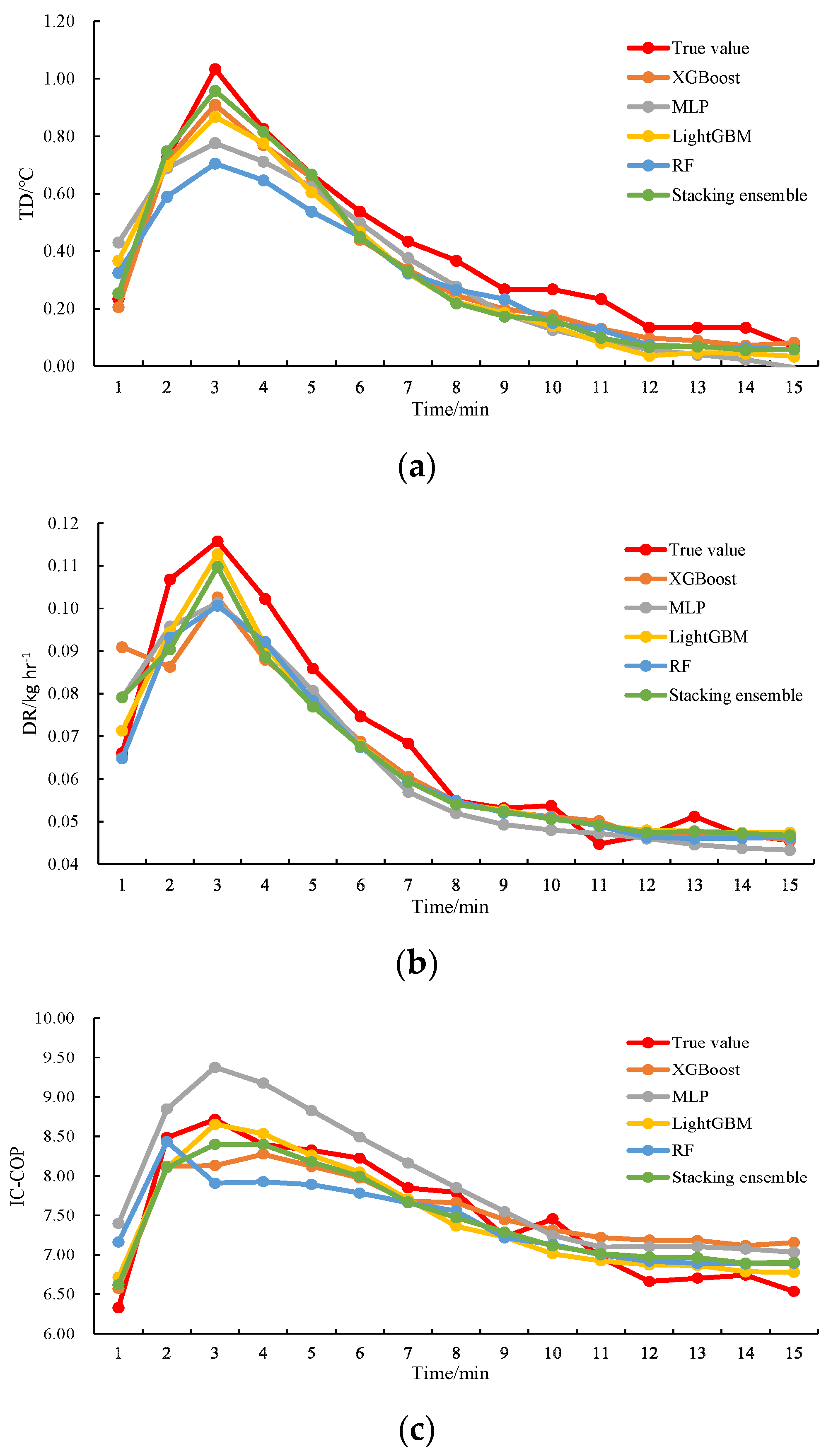
As shown in Figure 6a, due to the large temperature difference between indoor air and refrigerant at the beginning, TD showed a significant decrease in the first 0–10 min. In the following 10–14 min, the temperature drop was in a stable phase. In Figure 6b, DR initially exceeded 5 kg/h, and then dropped to 2.5–3.0 kg/h within 9–12 min. If it continued to operate, it would waste energy. Figure 6c showed that IC-COP slightly increased in the third minute, then continued to decrease until 10 min, and stabilized within 11–14 min. The average IC-COP of the system was 3.91. Among all models, especially the stacked model system, it exhibited the best tracking performance and effectively predicts fluctuations and stable phases.

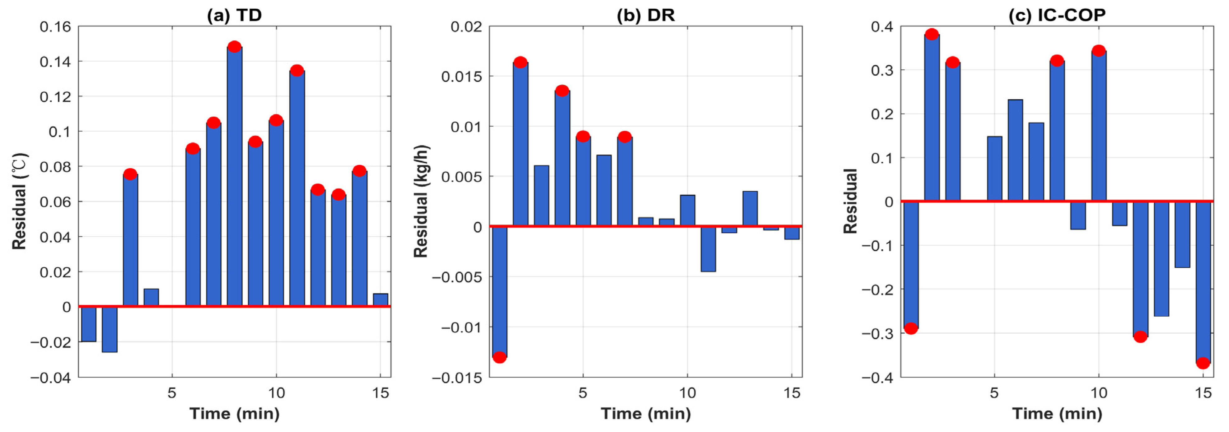
Stacking ensemble model’s residual analysis reveals significant differences in overall prediction performance: DR predictions are the most accurate, with a residual range of only −0.0131 to +0.0164 kg·h⁻¹, a mean close to zero, and a balanced distribution of positive and negative residuals (8 positive, 7 negative), indicating that the model effectively captures its variation patterns; TD predictions exhibit systematic positive bias, showing positive residuals and a residual range of −0.0258 to +0.1481 °C, particularly during the mid-phase rapid change period (6–11 min), where residuals significantly increase to 0.09–0.15 °C; IC-COP predictions show the largest fluctuations, with a residual range of −0.3687 to +0.3807, and display an obvious oscillatory pattern of alternating positive and negative residuals. Notably, substantial positive residuals of +0.38 and +0.34 occur at the 2nd and 10th minutes, while negative residuals of −0.31 and −0.37 appear at the 12th and 15th minutes, reflecting the model’s inadequacy in capturing dynamic turning points (Figure 7).

Overall, the model performs well in predicting steady-state or gently varying stages (e.g., DR data), with an average absolute residual below 0.01, but exhibits larger errors during rapid change phases and at extreme points.

4. Discussion

4.1. The Diversity and Generalization Ability of Ensemble Learning

The predictive results of this study clearly validated the outstanding effectiveness of the stacked ensemble learning framework in simulating the dynamic performance of complex humidity and heat systems. Its technological advantages can be attributed to its core design focusing on model diversity and generalization ability in the following two aspects:

(1) The advantages of heterogeneous foundational learners and the collaborative integration of meta-learners

The stacking ensemble learning framework developed in this study adopts a high-level architecture. At the basic learning level (first level), different heterogeneous models were adopted. The tree models are adept at capturing conditional dependencies and threshold-based interactions between features and are insensitive to the scale of numerical features [39,40]. MLP effectively approximates complex continuous function relationships through its nonlinear activation function [38]. This diversity ensures that at least one model can provide relatively reliable preliminary predictions during system dynamics, such as rapid cooling and nonlinear IC-COP fluctuations. The role of the second level is not just simple weighting, but learning the optimal combination strategy from these heterogeneous preliminary predictions using relatively simple models such as linear regression [31]. During the training process, meta-learners essentially construct a mapping function from the output of the base learner to the final truth value, dynamically balancing the predictive reliability of different models, achieving more refined technical results [25,43].

(2) The meta-feature generation mechanism based on K-fold cross-validation effectively controls the risk of overfitting

When generating features for training meta-learners, K-fold cross-validation method was used [46]. In each fold, the meta-features generated for each training sample come from the base model that was not directly trained on that specific sample, thereby reducing the risk of data leakage. The meta-features generated by this mechanism can more accurately reflect the generalization ability of each basic learner, rather than their memory ability. Therefore, the combination rules learned by meta-learners trained on this dataset are more focused on enhancing the model’s robustness to unknown data, rather than achieving perfect fitting on the training set. This is one of the fundamental reasons why stacked models exhibit higher stability and prediction accuracy.

4.2. Limitations and Boundary Conditions for Reliable Model Application

Although the stacking ensemble learning framework proposed in this study demonstrates outstanding predictive accuracy and robustness for the condensation dehumidification system under the investigated conditions, it is necessary to acknowledge its limitations and the boundary conditions required to ensure reliable application.

(1) Data dependence and awareness of operational boundaries

The performance of the model fundamentally depends on the quality and representativeness of the training data. The experimental conditions in this study were designed to cover the practical operating range of condensation dehumidification in livestock housing: an initial temperature difference of –20 to –5 °C, an air flow rate of 0.6 to 1.5 m/s, a refrigerant flow rate of 3 to 7 L/min, and consistently high indoor humidity (>90% RH).

It is important to note that this operating range aligns with the physical necessity for dehumidification. Scenarios with significantly lower humidity (e.g., RH < 70%) or smaller temperature differences generally fall outside the need for active dehumidification in such environments. Therefore, while the model’s predictive accuracy may decline when extrapolating beyond the trained parameter space, this limitation inherently aligns with the practical engineering boundaries within livestock housing.

(2) Dynamic response and real-time adaptability

The current model was validated on quasi-steady-state cycles and performs minute-level predictions based on prescribed input sequences. Its ability to handle highly transient dynamics—such as sudden changes in moisture load due to animal activity or rapid fluctuations in outdoor temperature—has not been explicitly tested. In practical applications requiring immediate control adjustments, integrating this predictive model into a Model Predictive Control (MPC) framework would be necessary, along with additional validation under dynamic conditions.

(3) Parameter-specific prediction consistency

The residual patterns reveal significant performance heterogeneity across output parameters. While DR predictions demonstrate high consistency with balanced residuals, TD exhibits systematic bias, and IC-COP shows pronounced oscillations—particularly at dynamic turning points. This inconsistency suggests that the model’s learned representations may not equally capture the underlying physical relationships for all system outputs. Such parameter-specific performance variation indicates that in practical deployment, the model may require targeted calibration or hybrid approaches to ensure uniform reliability across the complete system state prediction. These residual-based insights, combined with the operational and dynamic limitations, should inform the model’s application scope and guide future refinements, particularly in enhancing dynamic responsiveness and reducing parameter-specific biases.

5. Conclusions

5.1. Main Findings and Conclusions

This study designed and predicted a condensation dehumidification system that utilizes natural cold energy for enclosed livestock houses in cold climates. The main conclusions are as follows:

(1) A novel, energy-efficient condensation dehumidification system has been developed specifically for cold winter. It takes full advantage of the characteristics of natural low temperature in cold winter to achieve effective dehumidification with minimal indoor heat loss and low operational energy cost.

(2) A performance model of dehumidification system both with moisture and thermal balance model was developed. This model provides a critical tool for evaluating the system’s perform through three key indexes (room temperature drop, dehumidification rate, and internal circulation coefficient of performance).

(3) The data reveal two key operational insights: indoor relative humidity (>90%) exhibits strong positive correlations with both DR and IC-COP, indicating that the system performs more efficiently under high-humidity conditions. Meanwhile, the initial temperature difference (ranging from –20 to –5 °C in this work) shows a strong negative correlation with cooling capacity but a positive correlation with IC-COP, highlighting a critical trade-off. Proper control of this parameter is essential to balance dehumidification effectiveness, energy efficiency, and thermal stability.

(4) For performance prediction and control, a stacking ensemble model demonstrated enhanced accuracy (R² = 0.908) and reliability for offline performance assessment and control guidance. However, predictions vary by parameters: dehumidification rate remains stable, temperature exhibits systematic bias, and IC-COP fluctuates during transitions. For practical implementation, key variables—indoor temperature (15–20 °C), air flow rate (0.6–1.5 m/s), refrigerant flow rate (3–7 L/min), and initial air-refrigerant temperature difference—should be monitored at 1 min intervals. This enables the model to provide data-driven recommendations for adjusting control parameters to improve dehumidification performance while minimizing undesired temperature fluctuations over a 14-min operational cycle.

However, the successful application of stacking ensemble learning framework in real-world control systems requires addressing the outlined limitations—potentially through hybrid modeling, adaptive learning, or on-site calibration—to ensure reliability beyond the experimental conditions.

5.2. Future Work

While this study demonstrates the feasibility and predictive potential of the proposed condensation dehumidification system, several avenues for future work remain. First, field trials in actual livestock houses are needed to assess system robustness under real-world variations in stock density and management practices. Second, integrating the stacking prediction model into a model predictive control (MPC) framework could enable real-time optimization of pump and fan operation, further improving energy efficiency while maintaining environmental setpoints. Finally, future work should also focus on evaluating the economic viability of system deployment at different farm scales through comprehensive techno-economic analysis and exploring its integration with renewable energy sources or waste heat recovery systems to develop fully sustainable environmental management solutions for cold-climate livestock production.