Cyclic Movable Cultivation Rack with TIR-Based Supplemental Lighting for Hydroponic Barley Fodder

Abstract

Improving space use while reducing supplemental-lighting demand is important for compact hydroponic fodder production. We developed a cyclic movable cultivation rack with total internal reflection (TIR)-based supplemental lighting and evaluated its geometry, preliminary structural performance, device-level light distribution, and short-cycle crop response. Relative to a predefined double-sided static geometric reference, the cyclic configuration increased nominal tray cultivation area by 36.4%. A preliminary linear-static check under a 5850 N equivalent load gave a maximum von Mises stress of 108.8 MPa, maximum deformation of 3.307 mm, and a yield-based safety factor of 2.16 for Q235 steel. At comparable recorded input power, TIR increased mean PPFD by 93.1% within the prescribed 350 mm single-unit reference-plane grid. After calibration to reference-plane mean-PPFD equivalence, lighting-unit AC active power decreased from 25.41 to 13.10 W, a descriptive 48.4% reduction relative to the same lens-free WS2812-based prototype baseline. In cultivation, harvested fresh biomass differed by approximately 0.3%, and the retrospective one-sided confidence bound was compatible with an exploratory 5% engineering margin but not the stricter 2% sensitivity margin. The results support prototype feasibility while array-level canopy photon exposure, whole-facility energy performance, and long-term mechanical reliability require further validation.

1. Introduction

Plant factories provide controlled environments for stable year-round crop production by regulating light, temperature, humidity, CO₂, and water and nutrient supply and represent an important pathway toward intensive, standardized, and intelligent protected agriculture [1,2,3,4,5]. At the broader system level, dynamic optimization of resource inputs has also been proposed as a means of improving resource-use efficiency, product quality, and energy costs in vertical farming [6]. Modular and containerized plant factories are particularly relevant where internal space is constrained [7,8]. Hydroponic barley fodder has a short production cycle and rapidly forms a dense fodder mat, making it suitable for controlled-environment forage production and prototype equipment evaluation [9,10,11,12]. However, internal space is inherently limited in modular facilities, and conventional fixed multilayer racks generally require operator aisles for tray loading, management, and harvesting. Increasing cultivation density can therefore intensify access and spatial-layout constraints. At the same time, fully artificial-light production is electricity intensive, with lighting and environmental control accounting for a major proportion of operating energy demand [13,14,15,16]. Reducing lighting input alone, however, is not sufficient if crop production is adversely affected. The central engineering challenge is therefore to increase cultivation density and reduce supplemental-lighting electrical demand simultaneously without materially compromising harvested biomass.

Existing plant-factory equipment research has focused mainly on sowing, transplanting, cultivation-plate transport, and operational automation. Tong et al. [17] improved the transplanting efficiency of hydroponic leafy vegetables using a high-speed sparse-planting mechanism, while Jia et al. [18] developed an automated transport system that enabled automatic input, output, and interlayer transfer of planting plates in a plant factory, representing a logistics-oriented approach to reducing manual labor. Such studies primarily emphasize transport efficiency, positioning accuracy, and automation, whereas the loss of cultivation area caused by fixed access aisles in modular facilities has received less targeted structural attention. Although vertical multilayer cultivation increases crop output per unit floor area [19], increasing the number of layers and trays also makes internal access more difficult. A closed-loop pathway that circulates trays and concentrates loading and unloading at the rack end could reduce aisle requirements without requiring operators to enter the rack interior. However, full-load circulation remains influenced by the polygonal effect of chain drives, driving load, and structural deformation; these factors should therefore be considered during prototype mechanical design [20].

Artificial lighting is a major component of plant-factory energy use, and its energy performance depends not only on light-emitting diode (LED) efficacy but also on fixture layout, mounting distance, beam angle, target area, photoperiod, and dimming strategy [13,14,15,16,21,22,23]. In multilayer cultivation with short fixture-to-canopy distances, wide-angle LED emission can spill beyond tray boundaries and produce higher photosynthetic photon flux density (PPFD) at the center than at the edges. Previous studies have shown that close-canopy lighting, targeted lighting, and adjustable light distributions can reduce photon delivery to non-target regions while maintaining target light levels, thereby lowering lighting energy demand [24,25,26,27]. Freeform secondary optics can redistribute emitted rays according to source radiation characteristics and target-plane requirements [28,29,30], and optical simulations of plant factories and horticultural lighting-lens studies have shown that ray tracing and wavefront control can be used to optimize spatial light distributions [31,32]. At the operational level, joint optimization of daily light integral (DLI) targets and LED dimming strategies can also reduce lighting electricity consumption per unit yield [33]. Total internal reflection (TIR) lenses combine refractive and internally reflected ray paths and are well suited to constraining divergent LED light within compact spaces. Taken together, previous studies demonstrate the benefits of vertical cultivation, automated crop transport, targeted lighting, close-canopy lighting, and secondary optical redistribution, but these strategies have generally been evaluated in different engineering contexts. Limited information is available on prototypes that integrate a movable high-density rack with secondary optical control and evaluate spatial capacity, lighting electrical demand, and crop response within the same experimental framework (

Table 1. Representative vertical cultivation and related engineering studies relevant to the present prototype.

Study	Crop/System	Cultivation and Lighting Strategy	Representative Quantitative Finding	Relevance to the Present Study
Touliatos et al. [19]	Lettuce; vertical vs. horizontal hydroponics	Vertical cultivation compared with horizontal hydroponics	13.8-fold greater fresh yield and 20-fold more plants per occupied growing floor area in the tested geometry	Demonstrates spatial-density potential; does not address movable tray handling or lighting-energy optimization
Jia et al. [18]	Plant-factory cultivation plates	Automated input/output and interlayer transport	Transport success 92.5–96.0%; operational efficiency 176–317 plates h−1	Mechanical/logistics benchmark; crop and lighting-energy performance were not evaluated jointly
Sheibani et al. [25]	Lettuce; sole-source LED	Close-canopy lighting at constant PPFD	15 d LED electricity decreased from 40 to 20 kWh between 45 and 15 cm separations, with no significant fresh-biomass difference	Demonstrates crop-lighting-energy trade-off without a movable high-density rack
Yang et al. [12]	Hydroponic barley fodder	PPFD treatments of 0, 100, 200, and 300 μmol m−2 s−1	The 200 μmol m−2 s−1 treatment showed a favorable overall growth-quality response	Provides crop-specific light-intensity context; does not address rack configuration or secondary-optics energy reduction
Present study	Hydroponic barley fodder	Four-layer cyclic rack with TIR-based supplemental lighting	30 vs. 22 positions layer−1 (+36.4% nominal area); 25.41 to 13.10 W fixture active power under reference-plane calibration; only small harvested-biomass differences	Integrates spatial-capacity, device optical/electrical, and exploratory crop-response evidence within one prototype

).

This coupled density–lighting-energy–biomass trade-off therefore defines the central engineering question addressed in the present study.

To address this coupled engineering challenge, this study developed a modular hydroponic barley-fodder prototype integrating a cyclic movable cultivation rack with TIR-based supplemental lighting. The central research question was whether cultivation density could be increased while supplemental-lighting electrical demand was reduced without materially compromising harvested biomass. Accordingly, the objectives were to: (1) design a closed-loop chain-driven movable rack and quantify its tray-capacity and nominal cultivation-area gain relative to a predefined static geometric reference; (2) perform preliminary drive-system and structural design checks for prototype development; (3) characterize device-level near-field PPFD redistribution and lighting-unit AC input active power under lens-free and TIR conditions; and (4) conduct exploratory short-cycle cultivation tests to evaluate harvested biomass and lighting-subsystem energy performance under a reference-plane-calibrated lower-power TIR strategy.

For prototype-level interpretation, two author-defined exploratory engineering benchmarks were used: (i) a ≥30% increase in nominal tray cultivation area relative to the predefined static geometric reference, selected as a practically meaningful design target within the fixed facility envelope; and (ii) a ≥30% reduction in fixture-level AC input active power while satisfying the predefined ±5% reference-plane mean-PPFD equivalence criterion. These thresholds are study-specific engineering benchmarks rather than universally established or preregistered success criteria. The lighting benchmark was informed by reported reductions associated with targeted and close-canopy lighting [25,27], whereas no field-wide standard was identified for cultivation-area gain in this prototype configuration. Harvested fresh biomass was not evaluated against a preregistered success threshold; instead, after the experiment it was interpreted using a retrospective exploratory 5% non-inferiority margin relative to CK, with 2% and 10% margins examined as sensitivity bounds. Because no universal cultivation-area or biomass non-inferiority thresholds have been established for this prototype configuration, these benchmarks and the retrospective biomass margin are used only for exploratory prototype-level interpretation rather than as confirmatory pass/fail criteria.

The present work should therefore be interpreted as a preliminary prototype-level evaluation under the specific facility dimensions, rack geometry, lighting arrangement, crop cycle, and operating conditions described herein. It does not demonstrate commercial-scale throughput, whole-facility energy efficiency, long-term mechanical reliability, array-level canopy photon equivalence, or industrial economic feasibility; these aspects require dedicated scale-up and long-duration validation.

2. Materials and Methods

2.1. Overall Research Framework and Experimental Platform

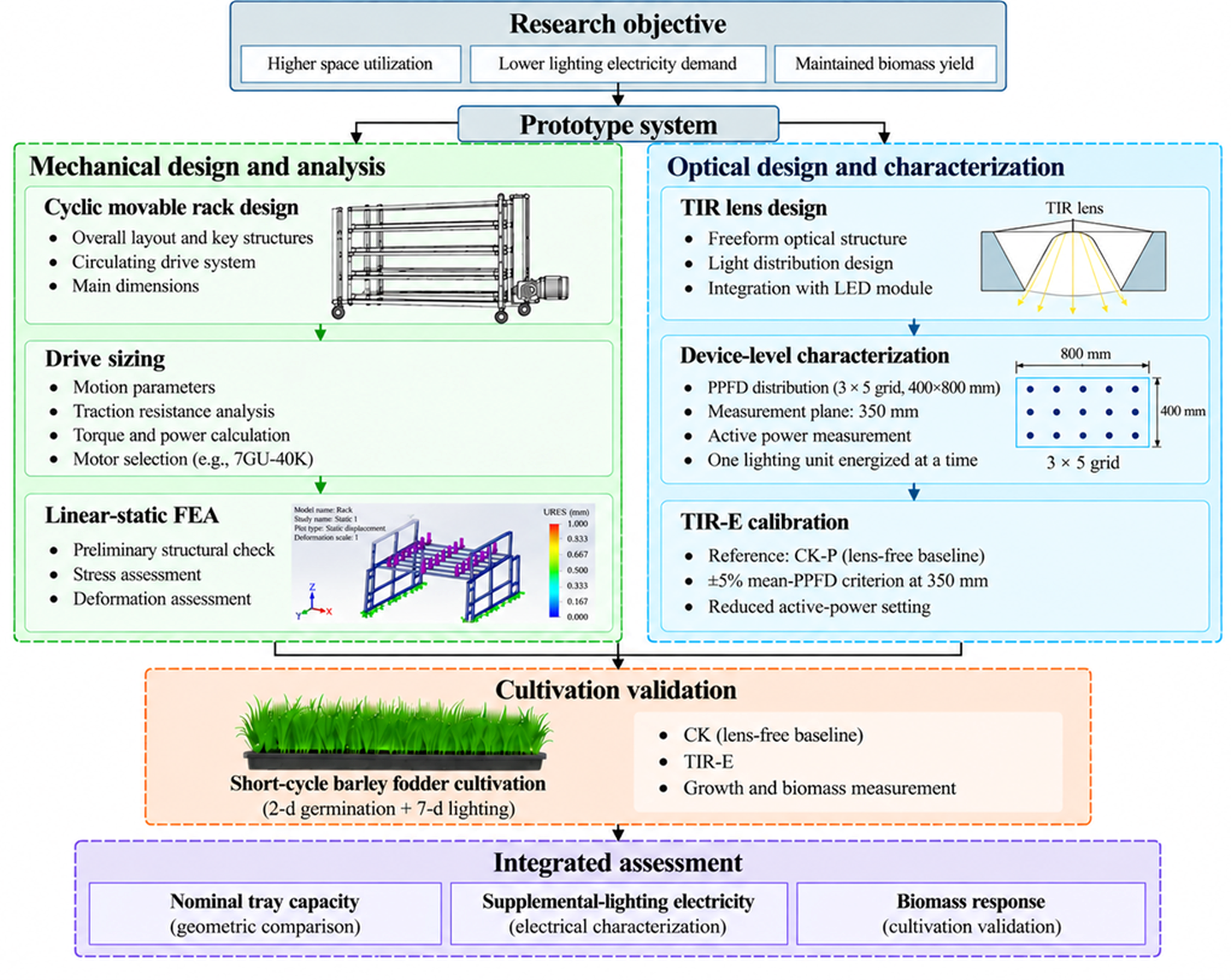
The study followed a four-stage engineering workflow organized around the coupled objective of increasing cultivation density and reducing supplemental-lighting electrical demand without materially compromising harvested biomass. The stages comprised: (i) prototype-system definition and cyclic-rack mechanical design; (ii) TIR-based optical-system design; (iii) device-level optical and electrical characterization followed by reference-plane calibration; and (iv) short-cycle hydroponic barley cultivation and statistical evaluation. Mechanical, optical/electrical, and cultivation evidence were analyzed at their respective experimental scales and were subsequently integrated for prototype-level engineering interpretation. The overall research framework and evidence flow are shown in Figure 1.

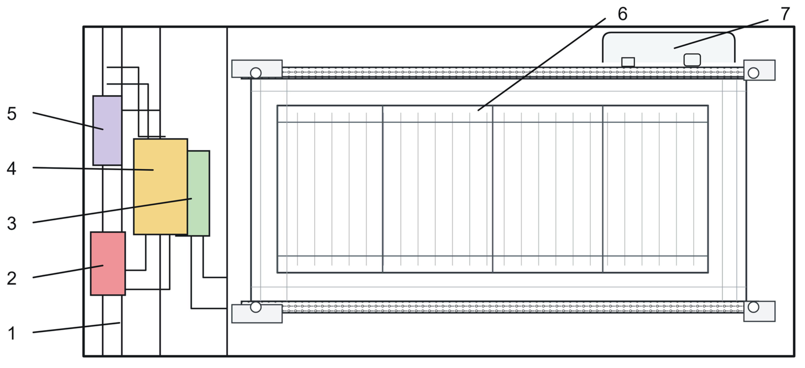
The experimental platform was located at the Smart Agricultural Equipment Innovation Center in the Yangling Demonstration Zone and was assembled on 14 February 2026. The plant factory was a fully artificial-light modular facility with external dimensions of 7000 mm × 3000 mm × 3000 mm and a floor area of 21 m². The interior was divided into cultivation and equipment zones. The cultivation zone contained a four-layer cyclic movable cultivation rack, an LED lighting system, and a recirculating spray nutrient-supply system, whereas the equipment zone contained refrigeration, fresh-air, recirculating-air, humidification, power-distribution, and centralized control equipment. Insulated sandwich panels were used as the enclosure to reduce the influence of external temperature fluctuations. The overall equipment layout is shown in Figure 2, and the main parameters are listed in

Table 2. Main parameters of the modular plant factory and cultivation rack.

Item	Parameter
Plant-factory external dimensions	7000 mm × 3000 mm × 3000 mm
Plant-factory floor area	21 m2
Cultivation-rack dimensions	6000 mm × 2560 mm × 1661 mm
Number of cultivation layers	4
Tray dimensions	850 mm × 400 mm × 40 mm
Trays per layer	30 designated cultivation positions (10 longitudinal × 3 transverse); chain return path not separately counted
Nominal longitudinal clear spacing between adjacent trays	220 mm
Supplemental lighting arrangement	28 columns along the rack length
Light source	WS2812 programmable RGB LED module (prototype source)
TIR lens material	PMMA, refractive index n = 1.49
Drive motor	7GU-40K DC variable-speed motor, 600 W, DC 24 V, maximum torque 120 N m

. A formal commissioning/stabilization log for the interval between assembly and the first cultivation batch was not retained in the available archive; therefore, no unverified stabilization duration is claimed in the present manuscript.

2.2. Design of the Cyclic Movable Cultivation Rack

2.2.1. Structural Components and Tray Loading/Unloading Procedure

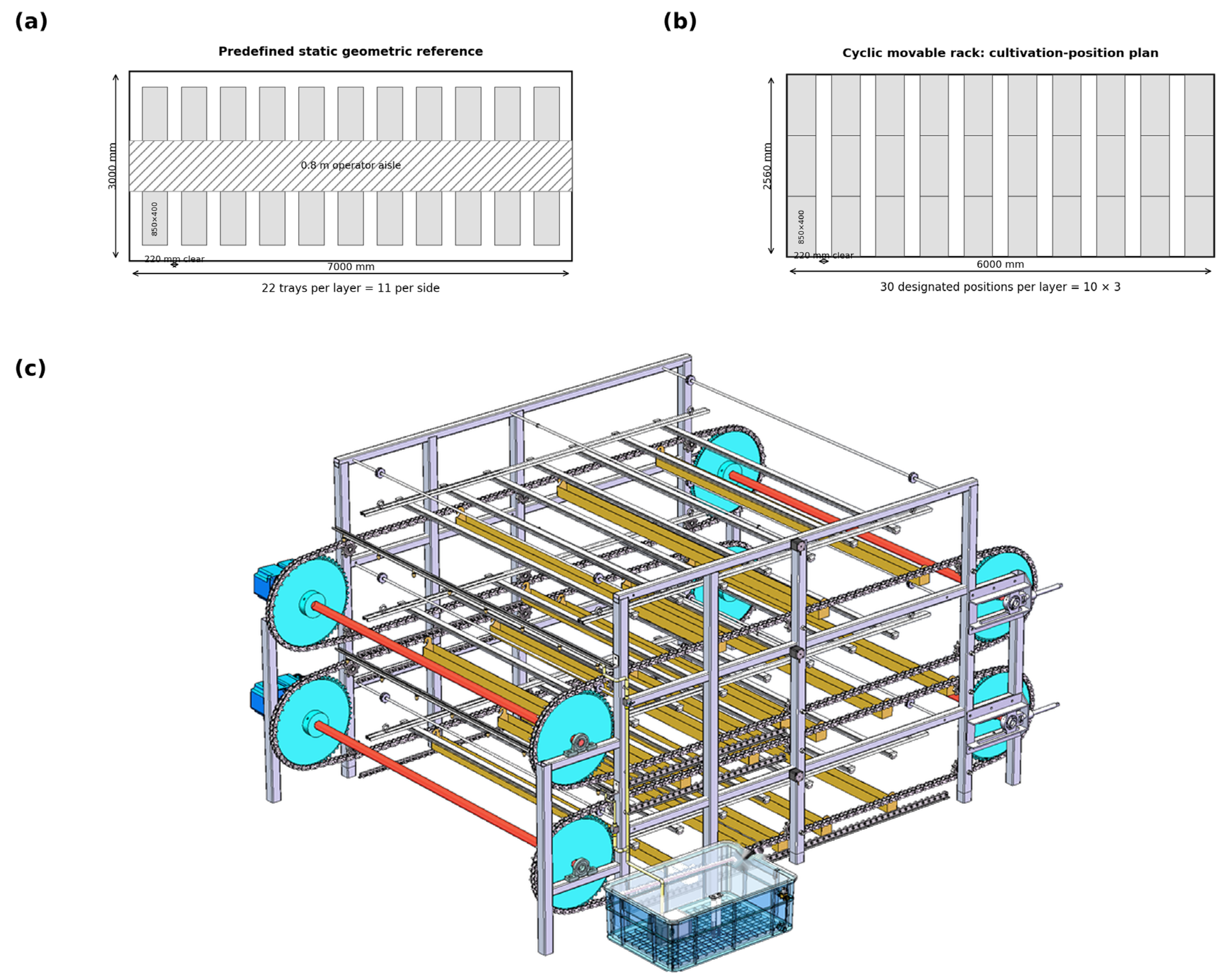
The cyclic movable cultivation rack consisted of a DC variable-speed motor, drive sprockets, idler sprockets, special conveyor chains, chain guide rails, screw-type tensioning units, suspended trays, and a square-steel load-bearing frame (Figure 3c). The main frame was welded from 50 mm × 50 mm × 2.5 mm square-steel tubing. During loading, operators placed trays sequentially at one end of the rack, and the chain-drive mechanism transported them to predetermined cultivation positions. After cultivation, the mechanism was restarted so that trays returned sequentially to the rack end for unloading. Thus, the cyclic drive was used for tray loading and unloading rather than for continuous circulation during the 7 d lighting period, when trays remained at their designated cultivation positions. Concentrating tray access at the rack end reduced the need for an internal operator aisle.

For the space-use comparison, a predefined conventional four-layer double-sided static layout used in the original facility design was adopted as a geometric reference configuration (Figure 3a). This reference was reconstructed dimensionally for design comparison and was not physically constructed or operated as a parallel experimental control in the present study. The same 850 mm × 400 mm trays were arranged on both sides of a 0.8 m central operator aisle with a nominal 220 mm clear longitudinal spacing between adjacent trays. With the 400 mm tray dimension oriented along the 7000 mm facility length, 11 trays and 10 intervening 220 mm gaps occupied 6600 mm on each side (11 × 400 + 10 × 220 = 6600 mm). Across the 3000 mm facility width, two 850 mm tray depths plus the 800 mm central aisle occupied 2500 mm. The predefined static geometric reference therefore accommodated 11 trays per side, or 22 trays per layer.

For the cyclic movable rack, the cultivation-position plan comprised 10 longitudinal positions × 3 transverse rows on each layer (Figure 3b). Along the 6000 mm rack length, 10 trays and nine nominal 220 mm gaps occupied 5980 mm (10 × 400 + 9 × 220 = 5980 mm). Across the 2560 mm rack width, three 850 mm tray rows occupied 2550 mm. Each layer therefore contained 30 designated horizontal cultivation positions. The 30-position count refers only to these tray positions occupied during the 7 d lighting period; chain-return portions required by the closed-loop drive were not counted as additional cultivation rows, additional tray positions, or additional illuminated cultivation area. All 30 designated positions were included in the tray-level lighting-energy allocation. Nominal tray cultivation area was defined as the summed horizontal plan area of occupied trays rather than the physical footprint of the rack. At 0.34 m² per tray, the static geometric reference provided 7.48 m² per layer and 29.92 m² across four layers, whereas the cyclic rack provided 10.20 m² per layer and 40.80 m² across four layers. The relative gain was (30 − 22)/22 × 100% = 36.4%. The cultivation-area-to-facility-floor-area ratio used the total plant-factory floor area of 21 m² as the denominator. Accordingly, the 36.4% value is a configuration-specific nominal spatial-capacity gain relative to this predefined geometry, not a theoretical maximum over all possible fixed-rack layouts and not an experimentally measured increase in crop productivity.

2.2.2. Chain-Drive Kinematic Analysis and Motor Selection

The polygonal effect of roller-chain drives can produce periodic variations in instantaneous chain velocity and may affect the stability of start–stop transport under full load [20]. For preliminary design screening, this effect was characterized using the following dimensionless chain-speed non-uniformity coefficient, k:

$$k={\displaystyle \frac{v_{\max }-v_{\min }}{v_{\max }}}=1-\cos \left({\displaystyle \frac{\pi }{z}}\right)$$

(1)

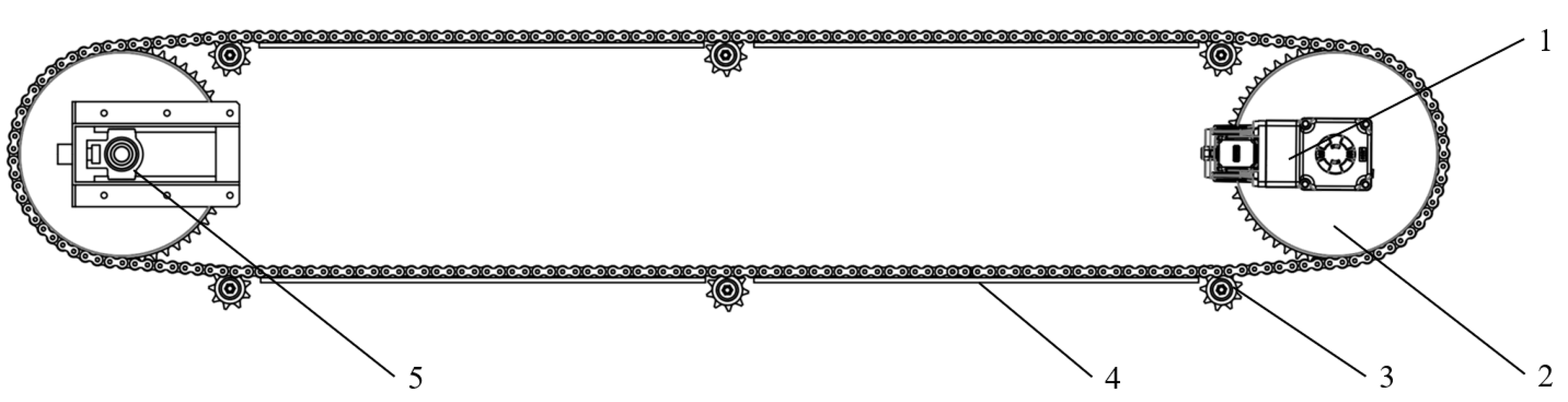
where vmax and vmin are the maximum and minimum instantaneous chain velocities, respectively, and z is the number of teeth on the drive sprocket. For z = 31, k = 1 − cos(π/31) = 0.0051, corresponding to 0.51%. This simplified index was used only to estimate the magnitude of polygon-induced speed fluctuation for preliminary design screening and was not intended to replace a full transient chain-drive analysis. The corresponding chain-drive arrangement is shown in Figure 4.

The archived chain-selection record identifies a 16A A-series extended-pin roller chain with an EP attachment, a nominal pitch of 25.4 mm, roller diameter of 15.8 mm, and chain mass of 2.66 kg m⁻¹. The same record lists a maximum allowable tension of 10.7 kN and, in its later strength check, a tensile strength of 55.6 kN. The dimensional and classification check in the present manuscript was updated against GB/T 1243-2024 [34]. Based on tray self-weight, mature fodder load, and chain and roller resistance, the total tractive resistance, F, was calculated as 480.52 N. Applying the operating-condition coefficient K = 1.3 gives a conservative design traction of 624.7 N. If this full design traction is assigned to one chain for screening, the ratio of the archived 10.7 kN allowable tension to design traction is 17.1. This value is treated only as a conservative static allowable-load margin and not as a fatigue, wear, impact, or dynamic chain safety factor. The required drive power and torque were calculated using Equations (2) and (3), respectively:

$$P={\displaystyle \frac{KFv}{\eta }}$$

(2)

$$T={\displaystyle \frac{KFd}{2\eta }}$$

(3)

where K is the operating-condition coefficient (1.3), v is the design mean chain velocity (0.6 m s⁻¹), η is the transmission efficiency (0.85), and d is the pitch diameter of the drive sprocket (0.251 m). The uncorrected tractive torque calculated from Fd/2 was 60.31 N m. After applying the operating-condition coefficient and transmission efficiency for motor sizing, the corrected design requirements were approximately 0.44 kW and 92.2 N m. A 7GU-40K DC variable-speed motor with a rated power of 600 W and a specified maximum output torque of 120 N m was selected. The 0.6 m s⁻¹ value was used for drive sizing rather than as evidence of continuous full-speed operation during cultivation. Because the selected DC drive was equipped with speed regulation, the prototype had the capability to operate below this sizing velocity during loading and unloading. However, acceleration/deceleration profiles, suspended-tray swing amplitude, and liquid-spillage events were not recorded quantitatively; therefore, 0.6 m s⁻¹ is not presented as a validated safe transport speed under all wet-load conditions.

2.2.3. Preliminary Linear-Static Finite-Element Design Check

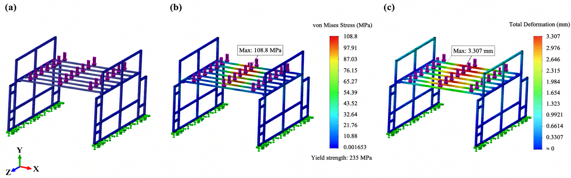
A linear-static finite-element analysis of the single-layer load-bearing support was performed in SolidWorks 2021 Simulation as a preliminary prototype-design check. The load-bearing structure was represented as a single continuous solid body, with the structural members treated as rigidly connected; therefore, no inter-component contact definitions were required. The structure was modeled as Q235 structural steel with an elastic modulus of 210 GPa, Poisson’s ratio of 0.30, density of 7.85 × 10³ kg m⁻³, and a yield strength of 235 MPa. The solid model was discretized using tetrahedral solid elements. The calculated maximum single-layer static load was 4286.52 N. A rounded basic static design load of 4500 N was adopted, and an operating-condition coefficient of 1.3 was applied to account conservatively for start-up impact and load fluctuation; accordingly, the final equivalent checking load used for the structural verification was 5850 N and was distributed over the modeled load-bearing region. Frame-support connection regions were represented by fixed constraints. Von Mises stress and total deformation were used as the principal structural-response indicators, and the yield-based safety factor was calculated using Equation (4). The analysis is interpreted as a preliminary linear-static design check of the continuous solid representation rather than as a detailed assessment of weld, joint, fatigue, or long-term structural behavior. The retained loading, boundary-condition, stress, and deformation contours are shown in Figure 5.

The load-bearing frame was analyzed as a single continuous solid body. The main rack frame uses 50 mm × 50 mm × 2.5 mm welded square steel members, and the completed SolidWorks 2021 Simulation study was a linear-static, small-displacement analysis. The standard solid mesher (Voronoi–Delaunay) was used consistently across all refinement levels, with high-quality 10-node second-order (parabolic) tetrahedral solid elements and a 16-point Gaussian Jacobian check. Automatic transition and solver settings were kept consistent across the mesh series. No inter-component contact definitions were required for the single-solid representation. The 5850 N equivalent checking load was applied as the total distributed load over the modeled load-bearing region, and the frame-support connection regions remained fixed. Global element sizes of 15, 10, 7.5, and 5 mm were evaluated, with nominal tolerances of 0.75, 0.50, 0.375, and 0.25 mm, respectively. Maximum von Mises stress and maximum total deformation were used as convergence indicators. The analysis was considered practically converged when the changes in both indicators between the two finest successive meshes were <5% and the locations of the response maxima remained stable (

Table 3. Numerical settings used for the completed linear-static finite-element analysis.

Parameter	Recorded Setting Used in the Completed Analysis
Model representation	Single continuous solid body; no inter-component contact pairs
Frame member geometry	50 mm × 50 mm × 2.5 mm welded square steel members
Software/study	SolidWorks 2021 Simulation; linear static; small-displacement formulation
Material model	Q235 structural steel; isotropic linear elastic; E = 210 GPa; ν = 0.30; ρ = 7.85 × 103 kg m−3; yield strength used for assessment = 235 MPa
Mesher	Standard solid mesher (Voronoi–Delaunay)
Element formulation	High-quality 10-node second-order (parabolic) tetrahedral solid elements
Jacobian check	16 Gaussian points
Global size sequence	15/10/7.5/5 mm
Tolerance sequence	0.75/0.50/0.375/0.25 mm nominally, corresponding to 5% of the respective global element sizes
Manual local mesh controls	None; only global element size was varied in the h-convergence series
Solver	Automatic solver selection
Boundary condition	Frame-support connection regions fixed
Applied load	Total distributed equivalent checking load = 5850 N
Gravity	Not separately activated in the completed reconstruction
Primary outputs	Maximum von Mises stress; maximum total deformation; yield-based safety factor
Mesh-quality acceptance	≥90% elements with aspect ratio <5; ≥90% with Jacobian ratio 1–10; no negative-Jacobian/distorted elements in accepted mesh
Mesh-convergence rule	<5% relative change in both maximum stress and maximum deformation between fine and very fine meshes, with stable maximum locations

and

Table 4. Mesh-convergence results for the four-level h-refinement series of the single-solid load-bearing structure.

Mesh Level	Global Element Size (mm)	Nodes	Elements	Maximum von Mises Stress (MPa)	Stress Change (%)	Maximum Total Deformation (mm)	Deformation Change (%)
Coarse	15	≈98,000	≈53,000	103.1	—	3.180	—
Medium	10	≈331,000	≈180,000	106.7	3.37	3.250	2.15
Fine	7.5	≈785,000	≈427,000	108.1	1.30	3.290	1.22
Very fine	5	≈2,650,000	≈1,440,000	108.8	0.64	3.307	0.51

).

$$n_s={\displaystyle \frac{{\sigma }_y}{{\sigma }_{\max }}}$$

(4)

For the four mesh levels, the recorded node/element counts were approximately 0.098/0.053 million, 0.331/0.180 million, 0.785/0.427 million, and 2.65/1.44 million, respectively. The recorded maximum von Mises stresses were 103.1, 106.7, 108.1, and 108.8 MPa, while the corresponding maximum total deformations were 3.180, 3.250, 3.290, and 3.307 mm. Relative to the next finer mesh, stress changes were 3.37%, 1.30%, and 0.64%, and deformation changes were 2.15%, 1.22%, and 0.51%. The fine-to-very-fine changes were below the 5% convergence criterion for both response quantities, with stable response-maximum locations. The 5 mm very-fine mesh was therefore treated as practically mesh-independent for this preliminary linear-static engineering check. The corresponding yield-based safety factor at 108.8 MPa was 235/108.8 = 2.16.

2.3. Design of TIR-Based Supplemental Lighting

2.3.1. Light-Distribution Requirements and Design Principle

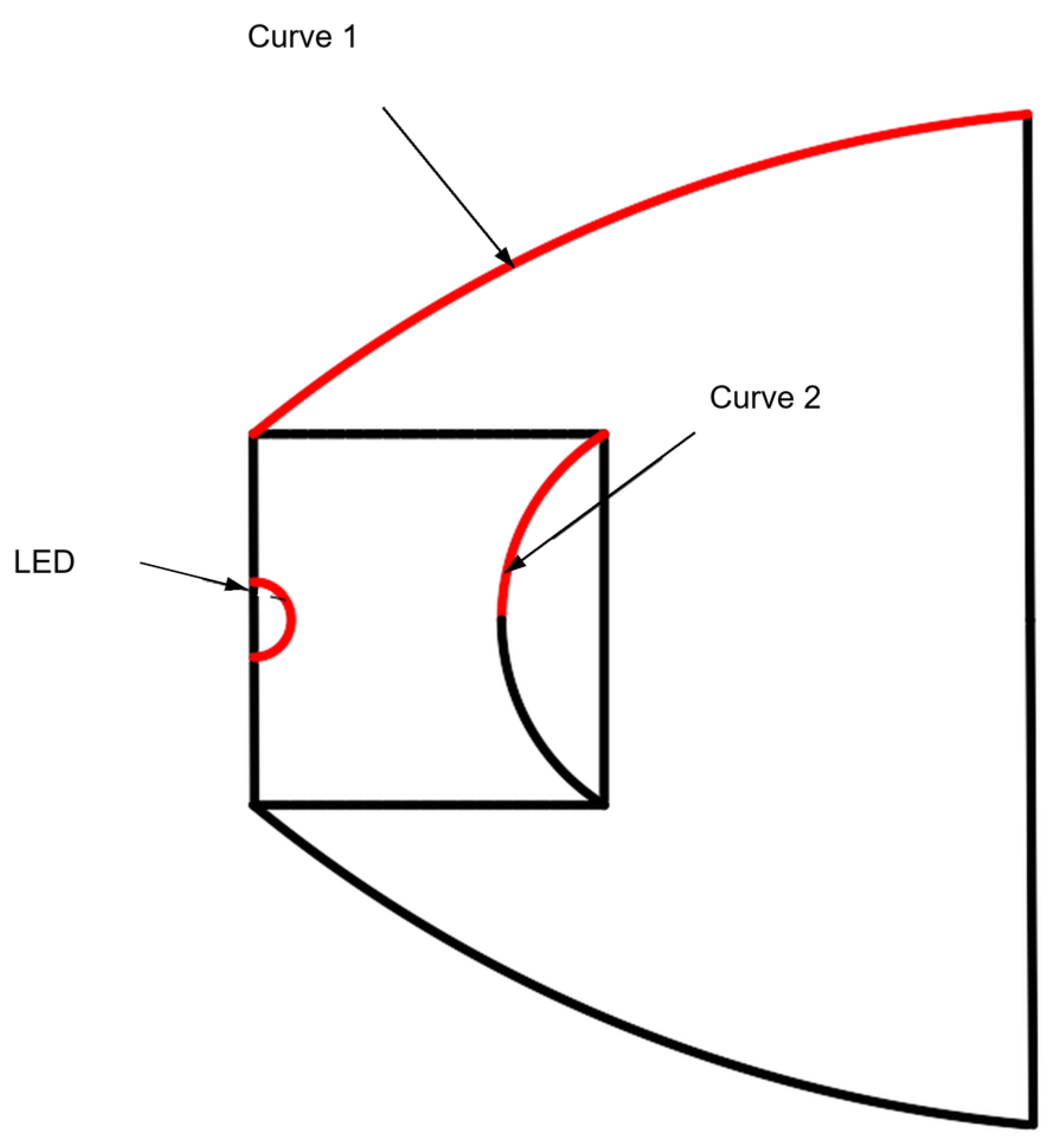
Programmable WS2812 red–green–blue (RGB) LED modules were used as the engineering prototype light source because independent channel control facilitated programmed RGB-channel control and synchronized pulse-width modulation (PWM) dimming during optical-system development. The modules were selected for controllable prototype development and were not intended to represent the photon efficacy, spectral optimization, thermal design, or optical architecture of a state-of-the-art commercial horticultural luminaire. Accordingly, CK-P should be interpreted as the lens-free baseline of this same WS2812-based prototype rather than as a generic horticultural-lighting benchmark. At short mounting distances, wide-angle LED emission can extend beyond the intended cultivation region and produce pronounced center-to-edge differences. To redistribute the emitted light toward the target plane, a TIR lens consisting of a refractive freeform surface and a total-internal-reflection freeform surface was designed (Figure 6). The refractive indices of polymethyl methacrylate (PMMA) and air were set to 1.49 and approximately 1.00, respectively, giving a critical angle of approximately 42.2°. Rays incident above the critical angle were redirected by the TIR surface, whereas near-axis rays were controlled by the refractive surface.

2.3.2. Freeform-Surface Construction and Optical Simulation

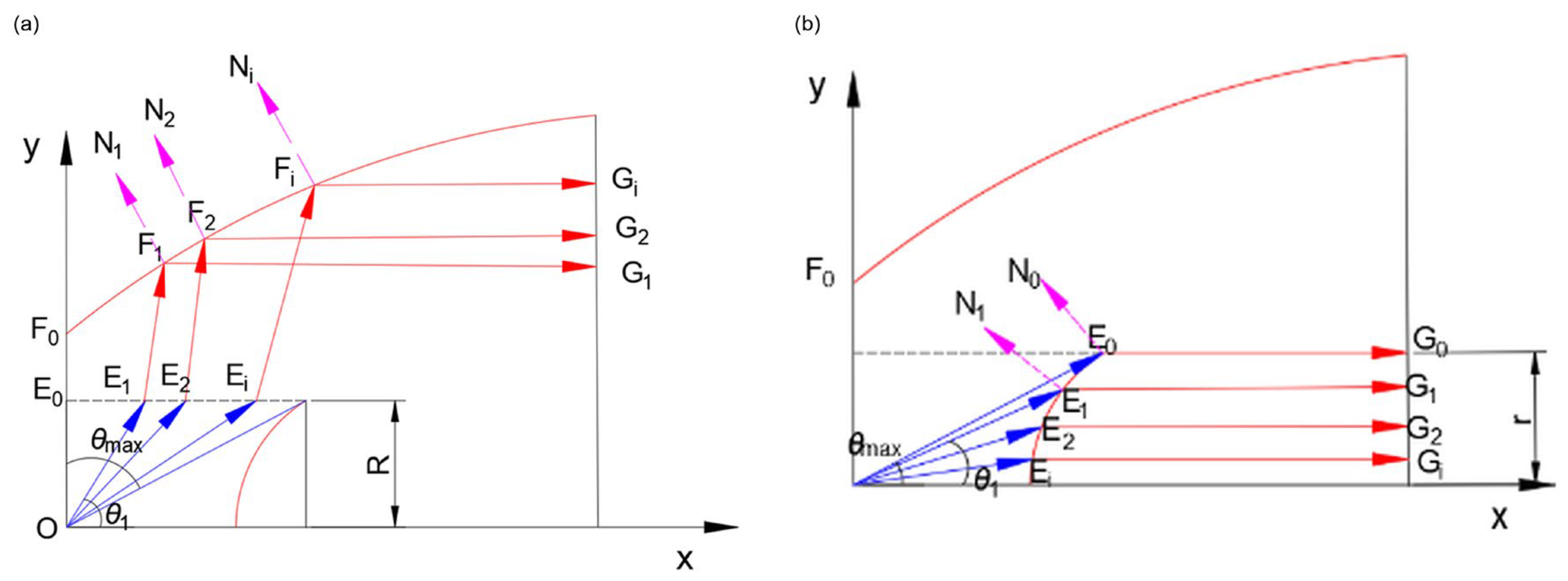
Based on energy conservation and the vector form of Snell’s law, the maximum LED emission angle was divided into N = 201 angular intervals, and the emitted optical flux in each interval was mapped to the corresponding region of the target plane. The freeform-surface normals and discrete coordinates were solved point by point, a generatrix was fitted using a cubic spline, and a three-dimensional lens model was then generated by revolution in SolidWorks 2021. The key design parameters are listed in

Table 5. Key design parameters of the TIR lens.

Parameter	Value
Lens material	PMMA (n = 1.49)
Maximum design incidence angle on the TIR surface	60°
Maximum design incidence angle on the refractive surface	30°
Number of angular divisions, N	201
3D modeling software	SolidWorks 2021
Optical simulation software	LightTools 2022.03

, and the surface-construction principle is illustrated in Figure 7.

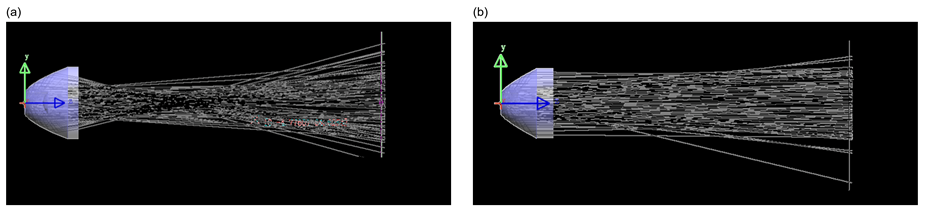
The three-dimensional lens model was exported in ACIS format and imported into LightTools for ray tracing. The simulations were used to compare the spatial distributions of the emitted rays before and after optimization (Figure 8).

2.3.3. Integrated Lighting-System Structure

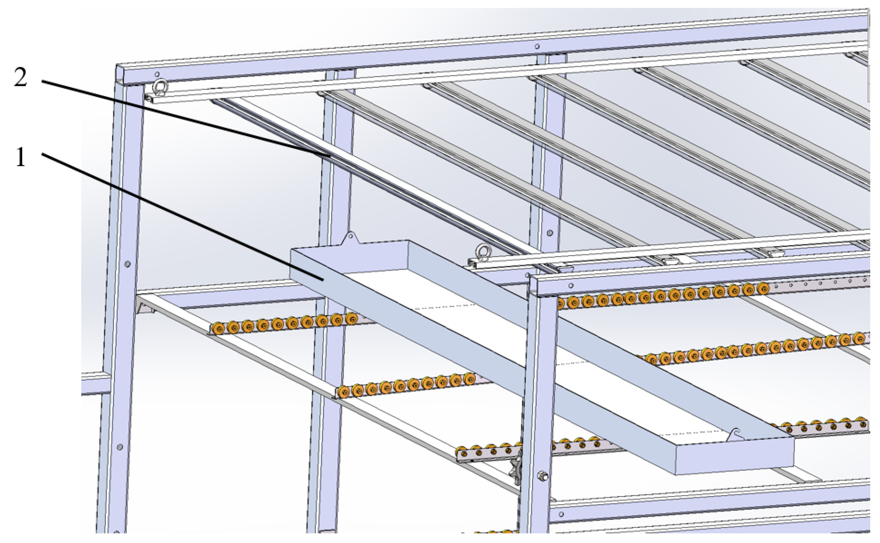
The supplemental lighting units were arranged in 28 columns along the 6000 mm length of the cultivation rack, with each column consisting of two 1100 mm light tubes connected in series. Each lighting unit comprised a heat sink, substrate, housing, RGB LED modules, and TIR secondary lenses. Based on the 2560 mm rack width, the nominal 60° LED beam angle, and the 350 mm optical reference distance, the required total tube length per column was calculated as approximately 2156 mm; therefore, a combined length of 2200 mm was adopted. The integrated arrangement of the supplemental-lighting units within the cyclic movable cultivation rack is shown in Figure 9.

The 350 mm optical reference distance and the angular parameters used in the lighting design were engineering parameters derived from the prototype geometry rather than crop-specific physiological optima. In the original fixture-layout design, the 2560 mm rack width, nominal 60° LED source beam angle, and 350 mm reference distance were used jointly to determine the required lighting-tube span. The nominal 60° source beam angle used for fixture layout should be distinguished from the 60° and 30° angular limits used in the freeform-lens construction; the latter define the ray domains assigned to the TIR and refractive portions of the lens. Likewise, the nominal 220 mm longitudinal inter-tray clearance was a configuration-specific mechanical/layout parameter selected to accommodate ten 400 mm tray positions within the 6000 mm rack length while retaining clearance for cyclic tray transport; it was not treated as an agronomically optimized spacing.

2.4. Device-Level Optical and Electrical Characterization

2.4.1. Lighting Conditions and Measurement Layout

Three lighting conditions were evaluated: a lens-free baseline (CK-P), a TIR condition operated at a practically comparable recorded input-power setting (TIR-P), and a lower-power TIR condition in which the red, green, and blue PWM duty cycles were synchronously reduced while maintaining the prescribed commanded channel-control ratio until mean PPFD on the reference plane satisfied the predefined ±5% engineering-equivalence criterion relative to CK-P (TIR-E) (

Table 6. Lighting conditions used in the device-level optical and electrical characterization.

Condition	TIR Lens	Power Setting	Primary Purpose
CK-P	No	Baseline operating setting (25.41 W recorded)	Establish the lens-free device-level reference field
TIR-P	Yes	Comparable recorded input-power setting (25.32 W)	Characterize near-field redistribution at comparable input power
TIR-E	Yes	PWM adjusted to the ±5% 350 mm reference-plane equivalence criterion (13.10 W recorded)	Evaluate descriptive fixture-level active-power reduction under reference-plane PPFD equivalence

). The “E” designation therefore refers specifically to reference-plane mean-PPFD equivalence and does not imply equality of instantaneous canopy PPFD or cumulative canopy photon exposure. Synchronous reduction of the commanded RGB duty cycles was intended to preserve the programmed channel ratio at the controller level; because no spectroradiometric spectral-power-distribution (SPD) measurement was performed, it is not treated as evidence that the emitted spectral shape remained invariant or that photon output from the three channels scaled linearly with duty cycle. The measurement objects were eight physically distinct lighting units from the same production batch. Because the TIR lens was installed at the individual-lighting-unit scale, these eight units were treated as device-level replicates for fixture characterization; between-unit variation represents manufacturing consistency rather than independent array-level treatment replication. Optical measurements were conducted one lighting unit at a time. A single unit was energized, allowed to stabilize, and measured before being switched off and the next unit was tested. For each unit, PPFD was recorded on a 3 × 5 grid with 200 mm point spacing, covering 400 mm in the across-rack direction × 800 mm in the along-rack direction. The grid was centered on the measured unit optical axis on a fixed horizontal plane 350 mm below the luminaire emitting surface. The 400 mm × 800 mm rectangle defines the spatial sampling domain only; it was not treated as the effective optical coverage area of a lighting unit and was not used to derive total photosynthetic photon flux (PPF) or photon efficacy. During crop cultivation, 28 lighting units operated simultaneously on each layer and neighboring illumination footprints overlapped. The single-unit maps were therefore not interpreted as the superposed array-level canopy light field; this scale distinction is illustrated in Supplementary Figure S2.

PPFD was measured with an LI-250A light meter equipped with an LI-190R cosine-corrected planar quantum sensor (LI-COR Inc., Lincoln, NE, USA), which measures photosynthetically active radiation in the 400–700 nm waveband. LI-COR technical documentation specifies factory calibration of the LI-190R against a standardized lamp traceable to NIST, an absolute calibration uncertainty of ±5%, and a recommended factory recalibration interval of 2 years. The sensor serial number and experiment-specific calibration-certificate date were not retained in the archived study records. The same sensor, grid geometry, stabilization procedure, and measurement protocol were used for all lighting conditions. No spectroradiometric measurement of the prototype RGB source was performed, and source-specific spectral-mismatch correction was not applied because the SPDs of CK-P, TIR-P, and TIR-E were unavailable. Accordingly, source-specific spectral-response error in the absolute PPFD values cannot be quantified from the retained data. Use of the same sensor and geometry makes some calibration-scale uncertainty common to the compared conditions, but it does not eliminate source-dependent spectral mismatch, particularly if the SPD changed with PWM operating point. The electrical operating values corresponded to the stabilized lighting conditions used for device-level characterization.

2.4.2. Electrical Measurement and Energy-System Boundary

Electrical input was characterized at the individual-lighting-unit level. For each optical condition, the 8962A1 multichannel power analyzer (Qingdao Qingzhi Instruments Co., Ltd., Qingdao, China) was connected at the AC input upstream of the complete lighting unit. According to the manufacturer’s current specification/manual, the 8962A1 has 0.1-class basic accuracy, a nominal measurement bandwidth of DC/0.5 Hz–300 kHz, 200 kS s⁻¹ simultaneous voltage/current sampling, selectable crest-factor settings (CF3/CF6), and functions for power factor and harmonic analysis. These specifications indicate that the instrument is designed for broadband and non-sinusoidal power measurements; however, the experiment-specific voltage/current ranges, crest-factor mode, line/filter settings, averaging/data-update interval, raw waveform records, and calibration certificate were not retained. The recorded active power therefore included the electrical demand of the LED source together with losses from the driver and local lighting-control electronics. The reported values of 25.41 W for CK-P, 25.32 W for TIR-P, and 13.10 W for TIR-E are retained AC-input active-power operating values rather than nominal or nameplate ratings. Because the original analyzer settings and repeated unit-level power time series could not be reconstructed, the retained electrical data support condition-level descriptive comparisons only; experiment-specific uncertainty for the PWM waveform cannot be quantified retrospectively. Power factor, crest-factor, current-harmonic and total-harmonic-distortion records were not retained, and compliance with GB 17625.1 is therefore not evaluated or claimed in this study.

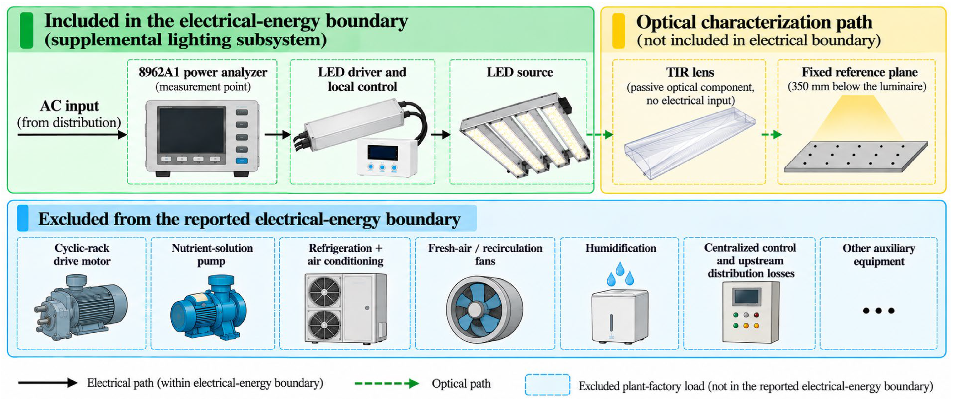
The complete modular plant factory contained multiple electricity-consuming subsystems, including supplemental lighting, the cyclic-rack drive motor, the recirculating spray/nutrient-supply system, refrigeration and air-conditioning equipment, fresh-air and recirculating-air fans, humidification equipment, power-distribution components, and centralized control hardware. The analyzer settings, calibration metadata, and repeated time-series records were not retained; therefore, the reported values are treated as condition-level descriptive active-power readings rather than as a complete uncertainty-characterized facility energy audit. However, the energy analysis reported in the present study was restricted to the supplemental-lighting subsystem. Within this boundary, the measurement point at the complete lighting-unit AC input included the LED source, driver losses, and local lighting-control electronics downstream of the analyzer. The TIR lens itself was a passive optical element and required no electrical input. Upstream power-distribution losses and the electrical demands of the cyclic-rack motor, nutrient-supply pump, refrigeration/air-conditioning equipment, ventilation fans, humidification system, and other facility-level auxiliary devices were not included in the reported lighting-energy metrics. Accordingly, all reported electricity-consumption and energy-productivity indicators are supplemental-lighting-subsystem metrics rather than whole-facility energy metrics. The reported electrical-energy boundary and its distinction from the downstream optical-characterization path are illustrated in Figure 10.

2.4.3. Calculation of Optical and Lighting-Energy Metrics

Spatial uniformity was characterized using three complementary metrics: the minimum-to-mean PPFD ratio (Umin/mean), the minimum-to-maximum PPFD ratio (Umin/max), and the coefficient of variation (CV). Umin/mean was retained as the primary uniformity metric following T/CSA 021-2013 [35], whereas Umin/max was additionally reported to describe the full minimum-to-maximum range of the sampled light field. All three metrics were calculated from the 15 grid positions within each lighting unit before summarization across the eight device-level replicates. ANSI/IES RP-45-21 was additionally consulted for horticultural-lighting terminology and target-plane evaluation context [36]; it is not used here to impose a separate numerical pass/fail threshold. Reporting Umin/mean, Umin/max, and CV in parallel avoids interpreting a single uniformity ratio as a complete description of the sampled PPFD field.

$$U_{\min /\mathrm{mean}}={\displaystyle \frac{{\mathrm{PPFD}}_{\min }}{{\mathrm{PPFD}}_{\mathrm{mean}}}}\times 100\%$$

(5)

$$U_{\min /\max }={\displaystyle \frac{{\mathrm{PPFD}}_{\min }}{{\mathrm{PPFD}}_{\max }}}$$

(6)

$$\mathrm{CV}={\displaystyle \frac{{\mathrm{SD}}_{\mathrm{PPFD}}}{{\mathrm{PPFD}}_{\mathrm{mean}}}}\times 100\%$$

(7)

Reference-plane daily light integral (DLIref), calculated 7 d lighting electricity consumption per lighting unit (E), and fixture-level active-power reduction (ηP) were calculated using Equations (8)–(10), respectively:

$${\mathrm{DLI}}_{\mathrm{ref}}={\displaystyle \frac{{\mathrm{PPFD}}_{\mathrm{mean}}\times 3600\times L}{{10}^6}}$$

(8)

$$E={\displaystyle \frac{P\times L\times D}{1000}}$$

(9)

$$\eta P={\displaystyle \frac{P_{\text{CK-P}}-P_{\text{TIR-E}}}{P_{\text{CK-P}}}}\times 100\%$$

(10)

where L is the daily photoperiod (16 h d⁻¹), D is the cultivation duration (7 d), and P is the recorded AC input active power of the lighting unit. DLIref is a nominal reference-plane DLI derived from PPFD measured on the fixed 350 mm optical reference plane and should not be interpreted as the cumulative DLI actually received by the developing canopy. No cumulative electrical-energy meter was used to determine full-cycle lighting electricity consumption. Instead, lighting electricity was calculated deterministically from the retained condition-level AC input active power and the prescribed operating schedule. This calculation assumes that each lighting unit operated at the retained active-power value throughout the prescribed photoperiod and does not incorporate start-up transients, temporal power drift, downtime, or auxiliary plant-factory loads. The 48.4% value from Equation (10) is therefore a deterministic fixture-level active-power comparison between TIR-E and the same lens-free prototype baseline and is not accompanied by a unit-level SD or confidence interval. Total fixture PPF was not measured using an integrating sphere, goniophotometric system, or full angular photometric method; therefore, fixture photosynthetic photon efficacy (PPE) and target-area photon-capture efficiency were not calculated from the discrete PPFD grid. In particular, mean PPFD multiplied by the nominal 400 mm × 800 mm sampling rectangle was not used to infer whole-fixture PPF or PPE because the grid represents a finite sampling domain rather than an integrating boundary for all emitted photons.

2.5. Hydroponic Barley Fodder Cultivation Test Under Reference-Plane-Calibrated Lighting Conditions

2.5.1. Plant Material and Cultivation Conditions

The hydroponic barley fodder cultivation experiment was conducted from 18 February to 31 March 2026 at the Smart Agricultural Equipment Innovation Center in the Yangling Demonstration Zone. Four independent batches were established at intervals of approximately 10 d, and each batch had a 9 d cultivation cycle. Spring two-row barley (Hordeum distichum) was used. Approximately 500 g of seed was sown per tray and spread uniformly to a depth of approximately 10 mm in 850 mm × 400 mm × 40 mm trays. Seeds were germinated for 2 d in darkness at 26 °C and a relative humidity of at least 80%. At the end of germination, shoots were approximately 5 mm high and total tray mass was approximately 0.75 kg. Trays were then transferred to the plant factory for 7 d of supplemental-light cultivation under a 16 h d⁻¹ photoperiod [37].

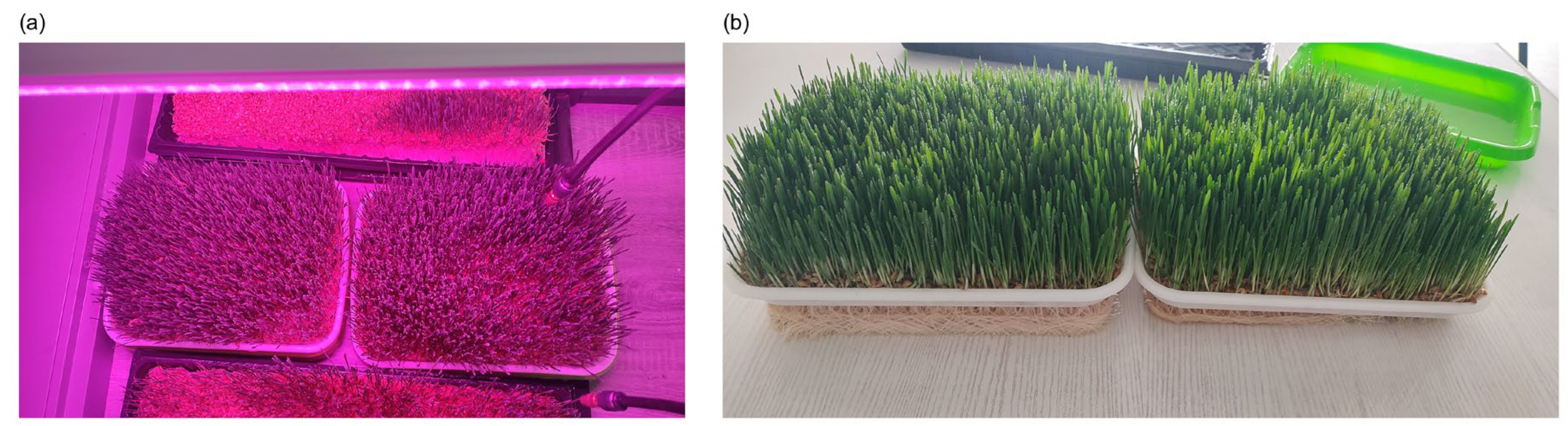
During supplemental-light cultivation, temperature was set to 26 °C and relative humidity was maintained at 70–80%. The luminaires were installed at the fixed prototype height corresponding to the 350 mm tray/reference-plane design distance and remained at that installation height throughout the 7 d lighting period; consequently, the actual luminaire-to-canopy distance decreased as the barley seedlings grew. CO₂ was managed within a nominal threshold range of 800–1200 ppm using the facility ventilation and environmental-control system; batch-specific device-actuation logs were not retained. All treatments used the same recirculating spray-hydroponic system and common nutrient-supply regime. The prototype irrigation system had been designed for a nominal spray cycle of 5 min every 2 h and incorporated reservoir liquid-level control and pH/EC sensing. However, batch-specific controller execution logs for the 2026 cultivation experiment were not retained, and the exact nutrient-solution formulation and time-resolved pH and EC records were unavailable. The 5 min/2 h schedule is therefore reported as the nominal system setting rather than as a continuously verified irrigation history for every batch. These missing nutrient-management records limit complete agronomic reproducibility, although CK and TIR-E were cultivated concurrently under the same shared management conditions within each batch. The cultivation environment and representative growth morphology are shown in Figure 11.

The principal crop-environment set points were selected with reference to published hydroponic barley and controlled-environment fodder studies rather than as independently optimized agronomic optima for this prototype. Because batch-specific nutrient formulation, pH/EC histories, and controller execution logs were not retained, these settings should be interpreted as nominal operating conditions and not as a fully reconstructable nutrient-management protocol. A PPFD near 200 μmol m⁻² s⁻¹ has been reported to provide a favorable balance of growth and nutritional quality in hydroponic barley fodder [12], and the approximately 215 μmol m⁻² s⁻¹ lens-free reference level measured in the present prototype was close to this range. A 16 h d⁻¹ photoperiod was selected because a dedicated barley-seedling photoperiod study identified 16 h d⁻¹ as suitable for plant-factory production [37]. The 26 °C temperature set point and 70–80% RH range were within conditions reported for controlled-environment hydroponic fodder production [9,12]. By contrast, the 350 mm reference distance, optical angular limits, and tray spacing described above were engineering design parameters rather than literature-defined physiological requirements for barley.

2.5.2. Experimental Design and Independent Replicates

The cultivation experiment compared a lens-free control (CK) with the TIR-E lower-power treatment calibrated according to the fixed 350 mm reference-plane mean-PPFD criterion. Four independent batches were conducted, with four cultivation layers used in each batch. Treatment assignment was not randomized. Instead, a predefined systematic alternating assignment (crossover-type layer schedule) was used so that CK and TIR-E exchanged layer positions between successive batches, reducing persistent confounding from fixed layer-specific microenvironments. Each batch × cultivation-layer combination was treated as one independent experimental unit, and three trays within each unit were treated as subsamples. Each treatment therefore comprised eight independent units and 24 trays, for a total of 48 trays. Because each batch × layer cell received only one treatment under this deterministic schedule, a batch × layer interaction cannot be estimated separately from residual variation; the statistical model therefore evaluates additive treatment, batch, and layer effects only. The systematic assignment schedule is shown in

Table 7. Systematic alternating (crossover-type) batch-by-layer treatment schedule in the hydroponic barley fodder cultivation experiment under the reference-plane-calibrated lighting strategy.

Batch	Layer 1	Layer 2	Layer 3	Layer 4
1	CK	TIR-E	CK	TIR-E
2	TIR-E	CK	TIR-E	CK
3	CK	TIR-E	CK	TIR-E
4	TIR-E	CK	TIR-E	CK

.

2.5.3. Growth Metrics and Lighting Energy Productivity

At the end of cultivation, 10 relatively uniform barley seedlings were randomly selected from each tray, and plant height was measured vertically from the point above the root system to the leaf tip; the tray mean was then calculated. For fresh-biomass measurement, the entire hydroponic barley fodder mat from each tray was removed and weighed immediately after visible continuous dripping had ceased. This value was defined as harvested fresh biomass per tray. After fresh weighing, the complete harvested material from each tray was placed in a forced-air oven, heated at 105 °C for 30 min, and then dried at 80 °C to constant mass to obtain harvested dry biomass per tray and dry-matter percentage. The three tray subsamples within each batch × cultivation-layer experimental unit were averaged before inferential analysis. Thus, the inferential sample size was n = 8 independent units per treatment; the 24 tray observations per treatment and the 10 seedling measurements within each tray were retained as lower-level subsamples and were not treated as additional independent replicates. For contextual discussion only, a literature-informed dry-matter recovery estimate was derived from the nominal seeding mass of approximately 0.500 kg tray⁻¹ using an assumed barley-seed dry-matter content of approximately 88% [38], corresponding to approximately 0.440 kg initial seed dry matter per tray. Initial seed dry matter was not measured directly, so this auxiliary estimate was not treated as a primary experimental endpoint or a directly measureed content.

Calculated lighting electricity consumption allocated per tray (E_tray), fresh-biomass energy productivity (EUE_fresh), dry-biomass energy productivity (EUE_dry), and specific lighting electricity consumption per unit fresh biomass (SEC_fresh) were calculated using Equations (11)–(14):

$$E_{\mathrm{tray}}={\displaystyle \frac{P_{\mathrm{group}}\times N_{\mathrm{group}}\times L\times D}{1000\times N_{\mathrm{tray}}}}$$

(11)

$${\mathrm{EUE}}_{\mathrm{fresh}}={\displaystyle \frac{M_{\mathrm{fresh}}}{E_{\mathrm{tray}}}}$$

(12)

$${\mathrm{EUE}}_{\mathrm{dry}}={\displaystyle \frac{M_{\mathrm{dry}}}{E_{\mathrm{tray}}}}$$

(13)

$${\mathrm{SEC}}_{\mathrm{fresh}}={\displaystyle \frac{E_{\mathrm{tray}}}{M_{\mathrm{fresh}}}}$$

(14)

where Pgroup is the recorded input active power of one lighting unit, Ngroup is the number of lighting units per layer (28), N_tray is the number of designated cultivation positions per layer (30), and Mfresh and Mdry are the harvested fresh and dry biomass per tray, respectively. During the 7 d lighting period, all 30 trays remained at the designated cultivation positions; the cyclic drive was not operated for continuous tray circulation. Thus, Ntray = 30 represents the number of simultaneously cultivated tray positions used for layer-level lighting-energy allocation. The cyclic-rack drive motor operated intermittently during tray loading and unloading. Because its cumulative operating time was not recorded during the cultivation experiment, actual drive electricity consumption could not be quantified retrospectively and was excluded from the lighting-energy metrics. Accordingly, the fixture-level active-power reduction and energy-productivity metrics in this study refer specifically to the supplemental-lighting subsystem rather than whole-system plant-factory electricity use. Because cumulative motor-on time was not logged, drive electricity is not added to the measured lighting-energy metrics.

2.6. Statistical Analysis

For the device-level optical characterization, lighting condition was treated as the within-unit fixed factor and physical lighting unit as the repeated-measures subject. Mean PPFD, Umin/mean, Umin/max, and CV were recalculated from the 15 raw PPFD grid values for each lighting unit before analysis. A one-factor repeated-measures ANOVA was applied to each device-level optical metric, with Greenhouse–Geisser correction for the omnibus test and Holm-adjusted paired comparisons for follow-up contrasts [39]. These tests quantify paired device-level differences among the eight measured fixtures and are not interpreted as independent array-level treatment replication. Before the optical experiment, a ±5% engineering-equivalence margin relative to the CK-P reference-plane mean PPFD was prespecified. CK-P versus TIR-E mean PPFD equivalence on the fixed 350 mm reference plane was evaluated using the two one-sided tests (TOST) framework [40], with the 90% confidence interval for the paired difference reported. For the cultivation experiment, the batch × cultivation-layer mean was the independent unit. Treatment, batch, and cultivation layer were entered as fixed categorical effects in a blocked linear model, Y ~ treatment + batch + cultivation layer, for plant height, harvested fresh biomass, harvested dry biomass, and dry-matter percentage. No random-effects or mixed-effects model was used; throughout the manuscript this analysis is therefore termed a blocked fixed-effects linear model. The treatment allocation was deterministic rather than randomized; because there was one treatment per batch × layer cell, the batch × layer interaction was not separately estimable and was not included in the additive model. With 16 independent-unit observations and eight fitted coefficients (intercept, treatment, three batch indicators, and three layer indicators), the residual degrees of freedom were 8. No prospective sample-size or statistical-power calculation was performed because the cultivation experiment was designed as exploratory engineering validation rather than a confirmatory agronomic efficacy trial. For harvested fresh biomass, the same blocked model was used for a retrospective exploratory non-inferiority analysis. A 5% loss relative to the CK mean was designated as the primary retrospective engineering margin, while 2% and 10% were retained only as stricter and more permissive sensitivity bounds, respectively. None of these biomass margins was prespecified before the experiment. Non-inferiority under an examined margin was considered supported when the one-sided 95% lower confidence bound for the adjusted TIR-E − CK difference exceeded the corresponding negative margin, following the confidence-interval logic used for non-inferiority reporting [41]. Residual normality was assessed using Shapiro–Wilk tests. Because the plant-height residual test indicated a mild departure from normality, the plant-height treatment effect was additionally examined using HC3 heteroskedasticity-robust standard errors while retaining the same blocked-model specification. All analyses were reproduced in Python 3.13.5 using NumPy 2.3.5, pandas 2.2.3, SciPy 1.17.0, and statsmodels 0.14.6. The significance level for two-sided tests was 0.05.

For the device-level optical analysis, Shapiro–Wilk tests applied to residuals from additive lighting-unit-plus-condition models gave W = 0.961 (p = 0.458) for mean PPFD, W = 0.927 (p = 0.0824) for Umin/mean, W = 0.986 (p = 0.976) for Umin/max, and W = 0.977 (p = 0.833) for CV; thus, no major residual-normality departure was detected for these four metrics. As a non-parametric sensitivity check, Friedman tests were also significant for all four optical metrics (χ² = 13.00, p = 0.00150 for mean PPFD and Umin/mean; χ² = 12.25, p = 0.00219 for Umin/max and CV), consistent with the Greenhouse–Geisser-corrected repeated-measures ANOVA. For the cultivation blocked models, residual Shapiro–Wilk results were W = 0.882 (p = 0.042) for plant height, W = 0.945 (p = 0.420) for harvested fresh biomass, W = 0.945 (p = 0.419) for harvested dry biomass, and W = 0.892 (p = 0.059) for dry-matter percentage. These diagnostic and sensitivity results are also reported in Supplementary Table S3.

Unless otherwise stated, continuous replicated outcomes are reported as mean ± standard deviation (SD), with n referring to the independent experimental unit at the corresponding evidence scale. For device-level optical metrics, n = 8 physical lighting units; for cultivation outcomes, n = 8 batch × cultivation-layer independent units per treatment, while tray and seedling measurements were subsamples rather than additional replicates. Input active power and calculated lighting electricity were retained as condition-level descriptive quantities and therefore were not assigned replicate-based SD, confidence intervals, or inferential significance labels. For cultivation outcomes, two-treatment inference is reported using blocked-model effect estimates, confidence intervals, and p-values rather than grouping letters. For the optical analysis, mean PPFD is reported without superscript grouping letters because the CK-P versus TIR-E scientific question is addressed primarily by the prespecified ±5% TOST equivalence analysis; conventional Holm-adjusted paired-difference p-values are reported in the text as secondary information. Superscript grouping letters are retained only for Umin/mean, Umin/max, and CV to summarize Holm-adjusted paired comparisons among the three optical conditions.

3. Results

3.1. Nominal Cultivation-Area Gain, Drive Design, and Preliminary Static Structural Check

Using the geometric definitions in Section 2.2.1 and Figure 3a,b, the predefined static reference provided 22 tray positions per layer, whereas the cyclic rack provided 30 designated cultivation positions per layer. This corresponds to a configuration-specific 36.4% increase in nominal tray cultivation area and an increase in the cultivation-area-to-facility-floor-area ratio from 1.42 to 1.94 (

Table 8. Nominal tray cultivation-area utilization and preliminary static structural-check results.

Metric	Predefined Static Geometric Reference	Cyclic Movable Rack/Verification Result
Tray positions per layer	22 (11 per side)	30 designated horizontal cultivation positions (10 × 3; return path excluded)
Nominal tray cultivation area per layer	7.48 m2	10.20 m2
Total nominal tray cultivation area, four layers	29.92 m2	40.80 m2
Relative nominal cultivation-area gain vs. geometric reference	—	36.4%
Cultivation-area-to-facility-floor-area ratio	1.42	1.94
Chain-speed non-uniformity coefficient	—	0.51%
Equivalent checking load	—	5850 N
Q235 yield strength used for assessment	—	235 MPa
Maximum von Mises stress	—	108.8 MPa
Maximum total deformation	—	3.307 mm
Yield-based safety factor	—	2.16

). No chain-return segment was counted as additional cultivated area. Because the static reference was not operated as a parallel cultivation treatment, this result represents a geometric capacity difference only and is not an experimentally measured difference in crop productivity or production throughput.

With a 31-tooth drive sprocket, the chain-speed non-uniformity coefficient was 0.51%. The uncorrected tractive torque was 60.31 N m, and the corrected design requirements used for motor sizing were approximately 0.44 kW and 92.2 N m; both remained below the selected motor ratings of 600 W and 120 N m. Under the 5850 N equivalent checking load, the preliminary linear-static analysis reported a maximum von Mises stress of 108.8 MPa and a maximum total deformation of 3.307 mm. Relative to the confirmed Q235 yield strength of 235 MPa, the corresponding yield-based safety factor is 2.16. These values describe the response of the single-continuous-solid idealization under the specified static checking condition and are not interpreted as experimental verification of weld behavior, fatigue resistance, or long-term structural reliability. The main results are summarized in Table 8.

3.2. Light-Redistribution Gain of the TIR Lens at Comparable Input Power

Greenhouse–Geisser-corrected repeated-measures ANOVA showed significant device-level effects of lighting condition on mean PPFD (F(1.04, 7.28) = 7815.06, p < 0.001), Umin/mean (F(1.54, 10.81) = 35.59, p < 0.001), Umin/max (F(1.37, 9.57) = 37.90, p < 0.001), and CV (F(1.67, 11.72) = 48.06, p < 0.001). The recorded input active powers used for CK-P and TIR-P were 25.41 and 25.32 W, respectively, differing by only 0.09 W (0.35%) and therefore representing practically comparable input-power settings for the optical comparison. At comparable measured input power, mean PPFD within the prescribed single-fixture near-field sampling grid increased from 215.03 ± 4.01 to 415.33 ± 10.48 μmol m⁻² s⁻¹, a device-level increase of 93.1%. Umin/mean increased from 84.92 ± 1.27% to 88.39 ± 1.12%, Umin/max increased from 0.628 ± 0.027 to 0.703 ± 0.012, and CV decreased from 14.14 ± 0.64% to 10.58 ± 1.12%. These results describe device-level near-field redistribution within the prescribed sampling domain.

Holm-adjusted paired comparisons showed conventional differences in mean PPFD among all three lighting conditions; however, mean PPFD is not assigned superscript grouping letters in

Table 9. Device-level optical metrics (n = 8 measured lighting units) and descriptive condition-level lighting-energy values under the three lighting conditions.

Condition	Mean PPFD (μmol m−2 s−1)	Reference-Plane DLI (mol m−2 d−1)	Umin/Mean (%)	Umin/max	CV (%)	Recorded AC Input Active Power (W)	Calculated 7 d Lighting Electricity per Unit (kWh)
CK-P	215.03 ± 4.01	12.39 ± 0.23	84.92 ± 1.27 b	0.628 ± 0.027 b	14.14 ± 0.64 a	25.41	2.85
TIR-P	415.33 ± 10.48	23.92 ± 0.60	88.39 ± 1.12 a	0.703 ± 0.012 a	10.58 ± 1.12 b	25.32	2.84
TIR-E	213.08 ± 5.51	12.27 ± 0.32	88.98 ± 0.99 a	0.712 ± 0.020 a	10.12 ± 0.63 b	13.10	1.47

Note: Optical metrics are reported as mean ± SD across eight device-level replicates. Each unit was measured while energized individually on the fixed 350 mm reference plane. The reported optical SD therefore quantifies device-to-device manufacturing variability rather than uncertainty in an array-level treatment mean. Umin/mean, Umin/max, and CV were calculated within each 15-point grid before summarization across units. Reference-plane DLI is a deterministic transformation of measured mean PPFD and was not tested separately. Input active power and calculated lighting electricity are reported descriptively at the condition level because unit-level raw power series were not retained; no inferential statistical test, SD, confidence interval, or grouping letter is applied to these quantities. Electricity consumption was calculated from the recorded AC input active power, a 16 h d⁻¹ photoperiod, and a 7 d cultivation period. TIR-P was used only for optical characterization and was not used for cultivation. For mean PPFD, no superscript letters are shown: the CK-P versus TIR-E comparison is interpreted primarily by the ±5% TOST equivalence analysis in Section 3.3, while conventional Holm-adjusted paired comparisons are reported as secondary results in the text. For Umin/mean, Umin/max, and CV only, means sharing the same superscript letter are not significantly different according to Holm-adjusted paired comparisons at α = 0.05.

because CK-P versus TIR-E is interpreted primarily using the prespecified equivalence framework reported in Section 3.3. For the three spatial-uniformity metrics, TIR-P and TIR-E did not differ significantly from one another, whereas both TIR conditions differed from CK-P. Grouping letters in Table 9 are therefore restricted to Umin/mean, Umin/max, and CV.

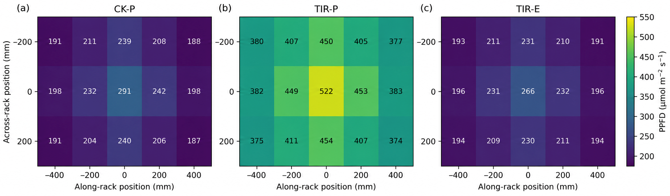
The spatial distribution across the 15 measurement points is shown in Figure 12. TIR-P increased PPFD at both central and peripheral grid positions relative to CK-P, although a higher-intensity central region remained. After PWM dimming, TIR-E retained a spatial pattern similar to TIR-P while reducing the mean PPFD to the CK-P reference level on the 350 mm plane.

Figure 12. Device-level PPFD distributions measured on the fixed 350-mm reference plane: (a) CK-P, the lens-free baseline; (b) TIR-P, the TIR condition operated at a comparable recorded input-power setting; and (c) TIR-E, the lower-power TIR condition calibrated to the ±5% reference-plane mean-PPFD equivalence criterion. Each panel represents the mean PPFD at the corresponding 3 × 5 grid position across eight physical lighting units measured individually, with only one unit energized at a time. The grid covered 400 mm in the across-rack direction × 800 mm in the along-rack direction with 200 mm point spacing. A common color scale is used across all three conditions. These maps characterize the near-field distribution of individual lighting units and should not be interpreted as the PPFD distribution of the 28-unit installed array or of the crop canopy during cultivation. Because the displayed maps are formed from pointwise means across the eight lighting units, a uniformity ratio recalculated directly from the displayed mean map can differ slightly from Table 9, where Umin/mean, Umin/max, and CV were first calculated within each 15-point unit-level grid and then summarized across units.

Figure 12. Device-level PPFD distributions measured on the fixed 350-mm reference plane: (a) CK-P, the lens-free baseline; (b) TIR-P, the TIR condition operated at a comparable recorded input-power setting; and (c) TIR-E, the lower-power TIR condition calibrated to the ±5% reference-plane mean-PPFD equivalence criterion. Each panel represents the mean PPFD at the corresponding 3 × 5 grid position across eight physical lighting units measured individually, with only one unit energized at a time. The grid covered 400 mm in the across-rack direction × 800 mm in the along-rack direction with 200 mm point spacing. A common color scale is used across all three conditions. These maps characterize the near-field distribution of individual lighting units and should not be interpreted as the PPFD distribution of the 28-unit installed array or of the crop canopy during cultivation. Because the displayed maps are formed from pointwise means across the eight lighting units, a uniformity ratio recalculated directly from the displayed mean map can differ slightly from Table 9, where Umin/mean, Umin/max, and CV were first calculated within each 15-point unit-level grid and then summarized across units.

3.3. Device-Level Reference-Plane PPFD Equivalence and Fixture-Level Active-Power Reduction

Mean PPFD on the fixed 350 mm device-level reference plane was 215.03 ± 4.01 μmol m⁻² s⁻¹ for CK-P and 213.08 ± 5.51 μmol m⁻² s⁻¹ for TIR-E. The paired TIR-E − CK-P difference was −1.95 μmol m⁻² s⁻¹ (paired-difference SD = 1.74 μmol m⁻² s⁻¹), corresponding to −0.91% of the CK-P mean. The 90% CI was −3.12 to −0.78 μmol m⁻² s⁻¹, and the entire interval lay within the prespecified ±5% engineering-equivalence margin (±10.75 μmol m⁻² s⁻¹; TOST p = 9.87 × 10⁻⁷). Thus, mean PPFD equivalence was supported only for the eight individually measured lighting units on the prescribed 350 mm reference-plane grid. No inference is made regarding whole-layer array PPFD, crop-canopy PPFD at different growth stages, or cumulative canopy photon exposure. The corresponding reference-plane DLI values were 12.39 ± 0.23 and 12.27 ± 0.32 mol m⁻² d⁻¹, respectively. The Holm-adjusted paired comparison nevertheless identified a small statistical difference in mean PPFD between CK-P and TIR-E (p = 0.0159). This is not contradictory to the TOST result: the conventional difference test evaluates whether the paired mean difference is distinguishable from zero, whereas TOST evaluates whether that difference remains within the prespecified ±5% engineering-equivalence bounds.

Under this reference-plane-calibrated condition, the recorded lighting-unit AC input active power decreased from 25.41 W for CK-P to 13.10 W for TIR-E, corresponding to a descriptive fixture-level reduction of 48.4% relative to the same lens-free WS2812-based prototype baseline. Calculated 7 d supplemental-lighting electricity consumption per lighting unit decreased from 2.85 to 1.47 kWh. Because the electricity values were calculated directly from the retained condition-level active-power values and a common operating schedule, the proportional decrease in calculated supplemental-lighting electricity was likewise 48.4%; this value does not represent whole-facility electricity reduction or a transferable efficiency gain for other horticultural luminaires. Because repeated unit-level power records were not retained, the 48.4% value is a deterministic condition-level comparison rather than an inferential estimate with quantified fixture-to-fixture uncertainty. TIR-E had Umin/mean = 88.98 ± 0.99%, Umin/max = 0.712 ± 0.020, and CV = 10.12 ± 0.63%. Detailed device-level comparisons are provided in Table 9.

3.4. Barley Fodder Production Performance Under the Reference-Plane-Calibrated Lighting Strategy

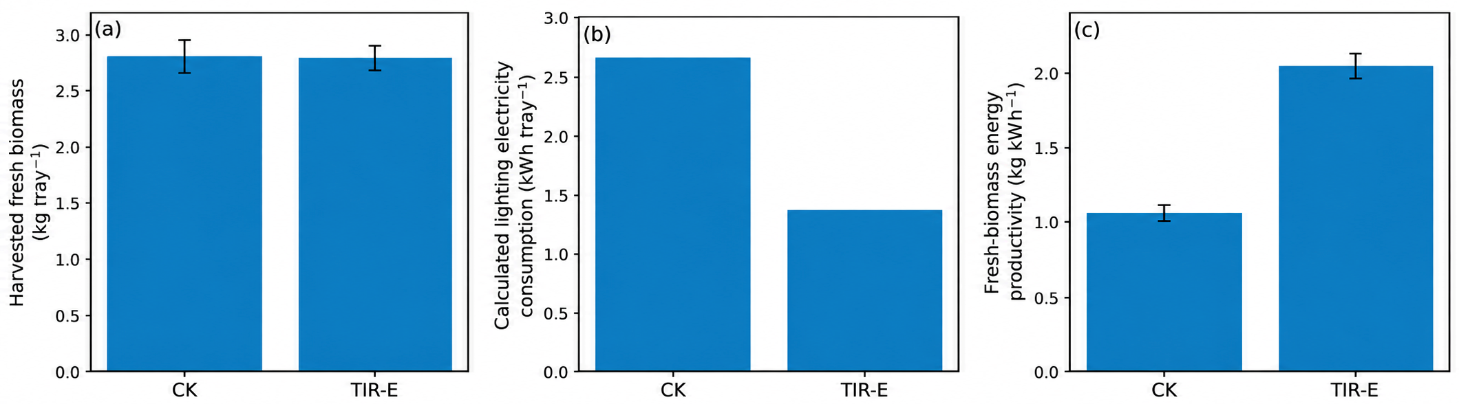
At the independent-unit level (n = 8 per treatment), plant height was 16.540 ± 0.493 cm for CK and 16.480 ± 0.419 cm for TIR-E, while harvested fresh biomass was 2.798 ± 0.144 and 2.789 ± 0.111 kg tray⁻¹, respectively. In the blocked linear models, the adjusted TIR-E − CK differences were −0.061 cm for plant height (95% CI, −0.441 to 0.319 cm; p = 0.722), −0.009 kg tray⁻¹ for harvested fresh biomass (95% CI, −0.129 to 0.110 kg tray⁻¹; p = 0.864), −0.0004 kg tray⁻¹ for harvested dry biomass (95% CI, −0.0128 to 0.0119 kg tray⁻¹; p = 0.939), and +0.018 percentage points for dry-matter percentage (95% CI, −0.301 to 0.338; p = 0.898). The plant-height residuals showed a mild departure from normality (Shapiro–Wilk W = 0.882, p = 0.042). In the HC3 robust-standard-error sensitivity analysis, the treatment estimate remained −0.061 cm, with robust SE = 0.233 cm, 95% CI = −0.598 to 0.477 cm, and p = 0.801. Thus, the interpretation of the very small plant-height effect was unchanged under the robust analysis. No plant-height equivalence margin was prespecified (

Table 10. Production performance of hydroponic barley fodder under the reference-plane-calibrated lighting strategy (mean ± SD of n = 8 batch × cultivation-layer independent units per treatment).

Metric	CK	TIR-E	Adjusted Difference (TIR-E − CK)	95% Confidence Interval	p-Value	Relative Change
Plant height (cm)	16.540 ± 0.493	16.480 ± 0.419	−0.061	−0.441 to 0.319	0.722	−0.4%
Harvested fresh biomass per tray (kg tray−1)	2.798 ± 0.144	2.789 ± 0.111	−0.009	−0.129 to 0.110	0.864	−0.3%
Harvested dry biomass per tray (kg tray−1)	0.3385 ± 0.0169	0.3381 ± 0.0164	−0.0004	−0.0128 to 0.0119	0.939	−0.1%
Dry-matter percentage (%)	12.101 ± 0.249	12.119 ± 0.309	+0.018	−0.301 to 0.338	0.898	+0.2%

Note: SD denotes standard deviation of the eight independent-unit means and is not SEM. Each independent unit contained three tray subsamples. For transparency, tray-level SDs (CK/TIR-E) were 0.641/0.564 cm for plant height, 0.162/0.152 kg tray⁻¹ for harvested fresh biomass, 0.0208/0.0234 kg tray⁻¹ for harvested dry biomass, and 0.354/0.424 percentage points for dry-matter percentage. Pooled individual-seedling SDs for plant height were 1.370/1.348 cm. Adjusted differences were estimated using linear models including batch and cultivation-layer blocking effects. Because the plant-height residual Shapiro–Wilk test gave p = 0.042, an HC3 robust sensitivity analysis was also performed; the treatment estimate was −0.061 cm (robust SE = 0.233 cm; 95% CI, −0.598 to 0.477 cm; p = 0.801).

).

3.5. Retrospective Exploratory Fresh-Biomass Non-Inferiority and Lighting-Energy Performance

Using the blocked fixed-effects linear model, the adjusted TIR-E − CK difference in harvested fresh biomass was −0.0092 kg tray⁻¹, and the one-sided 95% lower confidence bound was −0.1055 kg tray⁻¹, equivalent to −3.77% of the CK mean. Under the primary retrospective 5% engineering margin, this lower bound supported the interpretation that a loss greater than 5% was not indicated by the observed data. In sensitivity analyses, the lower bound also exceeded the −10% margin but did not exceed the stricter −2% margin. Thus, the data were compatible with the examined 5% retrospective engineering criterion, but not with the 2% sensitivity criterion. Because the 5% margin was selected after the experiment and no prospective sample-size calculation was performed, this analysis remains exploratory rather than confirmatory [41] (Table 11).

With 28 lighting units and all 30 designated cultivation positions occupied per layer during the lighting period, calculated 7 d supplemental-lighting electricity allocated per tray decreased from 2.66 kWh for CK to 1.37 kWh for TIR-E, corresponding to a 48.4% reduction in calculated supplemental-lighting electricity based on the retained condition-level active-power values. Fresh-biomass lighting-energy productivity increased from 1.05 to 2.04 kg kWh⁻¹ (+93.3%), dry-biomass lighting-energy productivity increased from 0.127 to 0.247 kg kWh⁻¹, and specific supplemental-lighting electricity consumption per unit fresh biomass decreased from 0.949 to 0.491 kWh kg⁻¹. These are supplemental-lighting-subsystem metrics and do not represent whole-facility energy efficiency. Harvested fresh biomass, allocated calculated supplemental-lighting electricity consumption, and fresh-biomass lighting-energy productivity are compared in Figure 13.

Table 11. Retrospective exploratory non-inferiority analysis of harvested fresh biomass per tray using the blocked linear model.

CK Mean (kg tray−1)	TIR-E Mean (kg tray−1)	Adjusted Difference (kg tray−1)	One-Sided 95% Lower Confidence Bound (kg tray−1)	Retrospective Exploratory Margin	Decision
2.798	2.789	−0.0092	−0.1055 (−3.77%)	−0.0560 (2% of CK; sensitivity)	Not met
2.798	2.789	−0.0092	−0.1055 (−3.77%)	−0.1399 (5% of CK; retrospective engineering margin)	Met
2.798	2.789	−0.0092	−0.1055 (−3.77%)	−0.2798 (10% of CK; sensitivity)	Met

Note: The effect direction is TIR-E − CK. The one-sided 95% lower confidence bound is based on the same blocked fixed-effects linear model used in Table 10, including batch and cultivation-layer blocking effects. The 5% loss margin is the primary retrospective engineering margin for interpretation; 2% and 10% are reported only as sensitivity bounds. None of the biomass margins was prespecified before the experiment, and no prospective sample-size calculation was performed for non-inferiority testing. Accordingly, the analysis is exploratory and should not be interpreted as a confirmatory non-inferiority trial [41].

Table 11. Retrospective exploratory non-inferiority analysis of harvested fresh biomass per tray using the blocked linear model.

CK Mean (kg tray−1)	TIR-E Mean (kg tray−1)	Adjusted Difference (kg tray−1)	One-Sided 95% Lower Confidence Bound (kg tray−1)	Retrospective Exploratory Margin	Decision
2.798	2.789	−0.0092	−0.1055 (−3.77%)	−0.0560 (2% of CK; sensitivity)	Not met
2.798	2.789	−0.0092	−0.1055 (−3.77%)	−0.1399 (5% of CK; retrospective engineering margin)	Met
2.798	2.789	−0.0092	−0.1055 (−3.77%)	−0.2798 (10% of CK; sensitivity)	Met

Note: The effect direction is TIR-E − CK. The one-sided 95% lower confidence bound is based on the same blocked fixed-effects linear model used in Table 10, including batch and cultivation-layer blocking effects. The 5% loss margin is the primary retrospective engineering margin for interpretation; 2% and 10% are reported only as sensitivity bounds. None of the biomass margins was prespecified before the experiment, and no prospective sample-size calculation was performed for non-inferiority testing. Accordingly, the analysis is exploratory and should not be interpreted as a confirmatory non-inferiority trial [41].

4. Discussion

4.1. Configuration-Specific Space-Use Gain and Evidence Boundary of the Static-Reference Comparison

The closed-loop chain drive concentrated tray loading and unloading at the rack end, permitting removal of the internal operator aisle assumed in the predefined static geometric reference. Under the specified facility envelope, tray dimensions, aisle width, and longitudinal spacing, the static reference accommodated 22 trays per layer, whereas the cyclic prototype provided 30 designated horizontal cultivation positions per layer, giving a configuration-specific 36.4% increase in nominal tray cultivation area. The comparison intentionally excludes chain-return portions from the cultivated-area numerator; those portions are part of the transmission path and were not treated as additional illuminated tray positions. Because the static layout was reconstructed from the original facility design and was not physically operated in parallel, the 36.4% value does not demonstrate an equivalent increase in realized yield, throughput, labor productivity, or whole-system efficiency. Those outcomes require a direct side-by-side comparison of operated static and cyclic systems under matched production conditions.

The corrected motor-sizing requirement was approximately 92.2 N m, below the 120 N m motor rating, and the corresponding design power of approximately 0.44 kW remained below the 600 W rating. The 0.51% polygon-effect coefficient provides only a preliminary kinematic indication. The completed multilevel mesh-refinement analysis indicated practical numerical convergence for the adopted linear-static model. Under the 5850 N equivalent checking load, the reported maximum stress of 108.8 MPa gives a yield-based safety factor of 2.16 against the confirmed 235 MPa yield strength. Numerical convergence does not replace physical validation of weld/joint behavior, start–stop dynamics, fatigue, tray swing, or long-term cyclic durability.

4.2. Spatial Redistribution of Target-Plane Light by the TIR Lens

At comparable recorded input-power settings, TIR-P increased the mean PPFD sampled within the single-fixture 3 × 5 near-field grid by 93.1% relative to CK-P. This result reflects redistribution of light on the prescribed reference plane rather than a 93.1% increase in total LED photon output or photon efficacy. Because the 15-point grid is a discrete sampling scheme rather than a spatial integration of the emitted photon field, mean PPFD multiplied by the nominal 400 mm × 800 mm sampling area cannot be used to estimate fixture PPF; consequently, PPE and target-area photon capture efficiency were not derived. The device-level evidence boundary is summarized in Supplementary Figure S2, consistent with prior work showing that secondary optics and close-canopy strategies can redistribute light at cultivation surfaces [24,25,26,27,28,29,30].

Spatial uniformity also improved but remained imperfect: Umin/mean increased from 84.92% to 88.39%, Umin/max from 0.628 to 0.703, and CV decreased from 14.14% to 10.58% from CK-P to TIR-P. A higher-intensity central region was still evident. At the 350 mm reference distance, the nominal 60° beam projects to approximately 404 mm in diameter, and the 28 simultaneously operating units per layer were expected to produce overlapping footprints. However, exact center-to-center spacing was not independently documented and simultaneous array-level PPFD mapping was not performed. Therefore, installed-array uniformity and canopy photon distribution cannot be inferred from the single-unit maps; these require array mapping at representative canopy heights together with total-PPF and spectroradiometric measurements.

4.3. Crop Response, Engineering Trade-Offs, and Lighting-Energy Performance

The ±5% optical equivalence result applies only to the fixed device-level reference plane 350 mm below individually measured luminaires. During cultivation, luminaire height was fixed while canopy height increased, and 28 lighting units operated simultaneously per layer. Reference-plane equivalence therefore does not establish identical instantaneous canopy PPFD, array-level PPFD, or cumulative canopy DLI, none of which was measured. Accordingly, the 48.4% reduction from 25.41 to 13.10 W is interpreted as a descriptive fixture-level reduction in recorded AC input active power under the predefined calibration criterion, not as proof of a 48.4% reduction in the electrical energy required to deliver an identical crop photon dose or in whole-facility electricity use. The magnitude is specific to the tested WS2812-based prototype and its lens-free baseline [21]. Because the CK-P source was an engineering prototype rather than a commercial horticultural luminaire, the observed percentage should not be generalized to luminaires that use different LED packages, driver efficiencies, thermal designs, spectral compositions, reflectors, lenses, or other secondary-optical systems. The present evidence therefore supports a prototype-specific benefit of redistributing the existing source output toward the prescribed reference plane; it does not establish a universal 48.4% energy-saving potential for commercial horticultural lighting.

PWM operation introduces an additional measurement boundary. The programmed synchronous reduction of the RGB duty cycles does not by itself prove invariant emitted SPD because the electrical-to-photon response of each color channel may differ with operating point. Likewise, although the 8962A1 is specified as a wide-band power analyzer with power-factor, crest-factor, and harmonic-analysis capability, the settings and waveform-quality outputs used in the present experiment were not archived. Consequently, the retained 25.41 and 13.10 W values are interpreted as descriptive AC-input active-power readings under the tested operating conditions, while power factor, harmonic compliance, and waveform-specific measurement uncertainty remain unresolved. No claim is made that the TIR-E operating point satisfies GB 17625.1. For the LI-190R measurements, absence of measured SPD also prevents source-specific spectral-mismatch correction; therefore, the absolute PPFD values carry an unquantified source-dependent component of uncertainty, although use of the same sensor and geometry reduces common calibration differences between conditions.

Crop response under the two reference-plane-calibrated lighting strategies showed only small differences. The fresh-biomass one-sided lower confidence bound was compatible with the retrospective 5% engineering margin but not the stricter 2% sensitivity margin, while dry biomass and dry-matter percentage also showed small adjusted differences with confidence intervals spanning zero. These biomass measurements do not establish equivalent forage nutritive value. In hydroponic barley fodder, light intensity has been reported to alter chlorophyll status as well as crude protein and fiber-related composition [12]; therefore, direct measurements of crude protein, NDF, ADF, ash, or related feeding-quality traits would be required before claiming nutritional equivalence between CK and TIR-E. Because the sample size was exploratory and the non-inferiority margins were not prespecified, the biomass results are not confirmatory proof of treatment equivalence. For context, harvested dry biomass of approximately 0.338–0.339 kg tray⁻¹ corresponds to an estimated dry-matter recovery of about 77% if the nominal 0.500 kg seeding mass and literature-based seed dry-matter content of approximately 88% are assumed [38]. This implies an estimated dry-matter loss of about 23%, similar in magnitude to the 21.9% loss reported by Dung et al. for 7 d hydroponic barley sprouting [42], but it is not a measured mass balance because initial seed dry matter was not determined. The retained current dataset contained complete harvest records for all 48 trays, but no standardized visible-mold/contamination score or microbiological assay was archived; consequently, hygienic performance cannot be inferred from the present dataset.

Within the defined supplemental-lighting boundary, calculated electricity allocated per tray decreased from 2.66 to 1.37 kWh and fresh-biomass lighting-energy productivity increased from 1.05 to 2.04 kg kWh⁻¹ (93.3%). The 12.31 W fixture-level difference corresponds to approximately 345 W per layer and 1.38 kW across four simultaneously illuminated layers. These values describe the lighting subsystem only. Motor, HVAC, pumps, humidification, ventilation, and other auxiliary loads were not metered over complete production cycles; therefore, neither the 48.4% fixture-level power reduction nor the 93.3% increase in lighting-energy productivity represents an equivalent change in whole-facility electricity use [15,16]. A possible reduction in cooling demand from the lower lighting load was not quantified. The 1.38 kW four-layer difference is an electrical-input difference rather than a measured HVAC-energy saving; actual cooling-energy reduction would depend on the chamber heat balance, HVAC coefficient of performance, and operating control, none of which was measured here.

The statistical and engineering interpretations should therefore be separated. The blocked model detected no fresh-biomass treatment effect (adjusted TIR-E − CK difference = −0.0092 kg tray⁻¹, approximately −0.3%; p = 0.864), but non-significance does not establish equivalence. The retrospective one-sided lower confidence bound corresponded to −3.77% of the CK mean, compatible with the examined 5% margin but not the 2% margin. At the prototype level, this small biomass difference occurred alongside a 36.4% configuration-specific increase in nominal tray cultivation area and a 48.4% fixture-level reduction in recorded active power relative to the same lens-free WS2812-based prototype baseline. The combination is encouraging as an engineering trade-off, but commercial gains in annual biomass productivity, whole-system energy efficiency, and economic return remain unverified.

4.4. Contextual Comparison and Economic Implications

Table 12. Multicriteria contextual comparison of representative vertical-cultivation, transport, and lighting-energy studies.

Study	Crop/System	Spatial/Mechanical Result	Crop Result	Energy Metric and Boundary
Touliatos et al. [19]	Lettuce; vertical vs. horizontal hydroponics	13.8-fold greater fresh yield and 20-fold more plants per occupied growing floor area in the tested geometry	Individual shoot fresh weight was lower in the vertical system	No directly comparable lighting-energy metric reported; spatial-density benchmark
Jia et al. [18]	Plant-factory cultivation-plate transport	92.5–96.0% transport success; 176–317 plates h−1	Crop production not evaluated	Energy not reported as a crop-energy metric; mechanical/logistics benchmark
Sheibani et al. [25]	Lettuce; close-canopy sole-source LED	No rack-density comparison	Fresh biomass did not differ significantly among the tested separation distances	15 d LED electricity decreased from 40 to 20 kWh between 45 and 15 cm separation; lighting subsystem
Pereira and Gomes [33]	Basil; vertical urban farm with natural + artificial light	No movable-rack capacity comparison	Average pot fresh biomass 32.5–47.5 g among DLI regimes	Potential LED specific electricity 1.64–4.90 kWh kg−1; hybrid natural/artificial-light boundary
Present study	Hydroponic barley fodder; four-layer cyclic rack + TIR	+36.4% nominal cultivation area vs. static geometric reference	2.798 vs. 2.789 kg fresh biomass tray−1 (CK vs. TIR-E); exploratory 5% margin compatible	2.66 to 1.37 kWh tray−1 and 0.949 to 0.491 kWh kg−1 fresh biomass; supplemental-lighting subsystem only

provides a non-weighted contextual comparison rather than a formal multicriteria decision-making ranking. A weighted AHP/TOPSIS-type analysis was not applied because the cited studies differ in crop species, production cycle, cultivation geometry, lighting source, environmental-control boundary, and energy-accounting method; common normalized criteria and defensible weighting factors were therefore unavailable. The table is intended to contextualize the evidence domains, not to claim superiority over the cited systems.

The cited studies consequently emphasize different evidence domains: verticalization primarily addresses production density, transport studies address logistics, and close-canopy or adaptive-lighting studies address crop–lighting-energy trade-offs. The present prototype integrates spatial capacity, secondary optical redistribution, fixture-level electrical demand, and short-cycle crop response within one platform. This integration should not be interpreted as overall superiority because the reported metrics do not share a common system boundary.

At 28 lighting units per layer, the 12.31 W difference between CK-P and TIR-E corresponds to approximately 154.4 kWh over one four-layer 16 h d⁻¹ × 7 d lighting period. Its direct monetary value would equal this calculated lighting-electricity difference multiplied by the applicable tariff. A reliable payback period cannot yet be estimated because incremental optical and rack capital costs, maintenance, replacement, motor electricity, and labor effects were not recorded systematically. Future economic assessment should therefore combine these costs with cumulative lighting-electricity savings and the economic value of the 32 additional nominal tray positions across four layers.

4.5. Limitations and Future Work

The principal limitations are defined by the evidence scales and retained records. Optical measurements were performed one lighting unit at a time on the fixed 350 mm reference plane and do not establish installed-array canopy PPFD, cumulative canopy DLI, whole-fixture PPF/PPE, or source-specific spectral equivalence. Exact nutrient formulation, time-resolved pH/EC records, and batch-specific controller logs were not retained; CK and TIR-E nevertheless received the same management within each batch, supporting relative comparison but not a fully reproducible agronomic protocol. The static rack was a reconstructed geometric reference rather than an operated control, and the fresh-biomass non-inferiority margin was retrospective and exploratory. Future work should prioritize (1) array-level canopy optical mapping and SPD characterization; (2) whole-facility energy metering; (3) dynamic start–stop, weld/joint, fatigue, and long-term full-load validation; and (4) broader agronomic, nutritional, hygienic, and economic assessment.

5. Conclusions

This study integrated a cyclic movable cultivation rack with TIR-based supplemental lighting for hydroponic barley fodder. Relative to the predefined static geometric reference, the cyclic layout provided a configuration-specific 36.4% increase in nominal tray cultivation area. The completed finite-element analysis should be interpreted as a preliminary linear-static design check; the observed mesh convergence does not constitute physical validation of long-term mechanical durability.

Under the tested reference-plane calibration, lighting-unit AC active power decreased from 25.41 to 13.10 W, corresponding to a descriptive 48.4% reduction relative to the same lens-free WS2812-based prototype baseline. The harvested fresh-biomass difference was small, but the retrospective non-inferiority analysis remained exploratory rather than confirmatory. These findings therefore indicate a potentially useful prototype-level engineering trade-off between nominal spatial capacity and supplemental-lighting electrical demand, but they do not demonstrate whole-facility energy saving or installed-array canopy equivalence. Future work should prioritize array-level optical validation, whole-facility energy measurement, dynamic mechanical testing, and broader agronomic, nutritional, hygienic, and economic assessment.

References

1. Qi, F.; Wei, X.; Zhang, Y. Current status and future research directions of protected-horticulture equipment technology in China. Trans. Chin. Soc. Agric. Eng. 2017, 33, 1–9. (In Chinese) [Google Scholar] [CrossRef]
2. Qi, F.; Li, K.; Li, S.; He, F.; Zhou, X. Development of intelligent equipment for protected horticulture worldwide and implications for China. Trans. Chin. Soc. Agric. Eng. 2019, 35, 183–195. (In Chinese) [Google Scholar] [CrossRef]
3. Avgoustaki, D.D.; Xydis, G. Plant factories in the water–food–energy nexus era: A systematic bibliographical review. Food Secur. 2020, 12, 253–268. [Google Scholar] [CrossRef] [Scilit]
4. Kozai, T. (Ed.) Smart Plant Factory: The Next Generation Indoor Vertical Farms; Springer: Singapore, 2018. [Google Scholar] [CrossRef] [Scilit]
5. Bantis, F.; Chatzigeorgiou, I.; Sismanis, M.; Ntinas, G.K. Vegetable production in PFALs: Control of micro-environmental factors, principal components and automated systems. Agriculture 2024, 14, 642. [Google Scholar] [CrossRef] [Scilit]
6. Kaiser, E.; Kusuma, P.; Vialet-Chabrand, S.; Folta, K.; Liu, Y.; Poorter, H.; Woning, N.; Shrestha, S.; Ciarreta, A.; van Brenk, J.; et al. Vertical farming goes dynamic: Optimizing resource use efficiency, product quality, and energy costs. Front. Sci. 2024, 2, 1411259. [Google Scholar] [CrossRef] [Scilit]
7. He, L.; Fu, L.; Fang, W.; Sun, X.; Suo, R.; Li, G.; Zhao, G.; Yang, R.; Li, R. IoT-based urban agriculture container farm design and implementation for localized produce supply. Comput. Electron. Agric. 2022, 203, 107445. [Google Scholar] [CrossRef] [Scilit]
8. Nikolov, N.V.; Atanasov, A.Z.; Evstatiev, B.I.; Vladut, V.N.; Biris, S.-S. Design of a small-scale hydroponic system for indoor farming of leafy vegetables. Agriculture 2023, 13, 1191. [Google Scholar] [CrossRef] [Scilit]
9. Ahamed, M.S.; Sultan, M.; Shamshiri, R.R.; Rahman, M.M.; Aleem, M.; Balasundram, S.K. Present status and challenges of fodder production in controlled environments: A review. Smart Agric. Technol. 2023, 3, 100080. [Google Scholar] [CrossRef] [Scilit]
10. Pastorelli, G.; Serra, V.; Turin, L.; Attard, E. Hydroponic fodders for livestock production—A review. Ann. Anim. Sci. 2024, 24, 645–656. [Google Scholar] [CrossRef] [Scilit]
11. Ceci, L.; Cavalera, M.A.; Serrapica, F.; Di Francia, A.; Masucci, F.; Carelli, G. Use of reclaimed urban wastewater for the production of hydroponic barley forage: Water characteristics, feed quality and effects on health status and production of lactating cows. Front. Vet. Sci. 2023, 10, 1274466. [Google Scholar] [CrossRef] [Scilit] [PubMed]
12. Yang, J.; Sun, J.; Wang, X.; Zhang, B. Light intensity affects growth and nutrient value of hydroponic barley fodder. Agronomy 2024, 14, 1099. [Google Scholar] [CrossRef] [Scilit]
13. Bu, K.; Yu, Z.; Lai, D.; Bao, H. Energy-saving effect assessment of various factors in container plant factories: A data-driven random forest approach. Clean. Energy Syst. 2024, 8, 100122. [Google Scholar] [CrossRef] [Scilit]
14. Cai, W.; Bu, K.; Zha, L.; Zhang, J.; Lai, D.; Bao, H. Energy consumption of plant factory with artificial light: Challenges and opportunities. Renew. Sustain. Energy Rev. 2025, 210, 115235. [Google Scholar] [CrossRef] [Scilit]
15. Stanghellini, C.; Katzin, D. The dark side of lighting: A critical analysis of vertical farms’ environmental impact. J. Clean. Prod. 2024, 458, 142359. [Google Scholar] [CrossRef] [Scilit]
16. Miserocchi, L.; Franco, A. Benchmarking energy efficiency in vertical farming: Status and prospects. Therm. Sci. Eng. Prog. 2025, 58, 103165. [Google Scholar] [CrossRef] [Scilit]
17. Tong, J.; Meng, Q.; Gu, S.; Wu, C.; Ma, K. Design and experiment of a high-speed sparse-planting mechanism for greenhouse hydroponic leafy vegetables. Trans. Chin. Soc. Agric. Eng. 2021, 37, 1–9. (In Chinese) [Google Scholar] [CrossRef]
18. Jia, D.; Guo, W.; Wang, L.; Zheng, W.; Gao, G. Design and experiment of automatic transport system for planting plate in plant factory. Agriculture 2024, 14, 488. [Google Scholar] [CrossRef] [Scilit]
19. Touliatos, D.; Dodd, I.C.; McAinsh, M. Vertical farming increases lettuce yield per unit area compared to conventional horizontal hydroponics. Food Energy Secur. 2016, 5, 184–191. [Google Scholar] [CrossRef] [Scilit] [PubMed]
20. Fuglede, N.; Thomsen, J.J. Kinematics of roller chain drives—Exact and approximate analysis. Mech. Mach. Theory 2016, 100, 17–32. [Google Scholar] [CrossRef] [Scilit]
21. Kusuma, P.; Pattison, P.M.; Bugbee, B. From physics to fixtures to food: Current and potential LED efficacy. Hortic. Res. 2020, 7, 56. [Google Scholar] [CrossRef] [Scilit] [PubMed]
22. Liu, X.; Sun, Q.; Wang, Z.; He, J.; Liu, X.; Xu, Y.; Li, Q. Innovative application strategies of light-emitting diodes in protected horticulture. Agriculture 2025, 15, 1630. [Google Scholar] [CrossRef] [Scilit]
23. Jin, W.; Formiga Lopez, D.; Heuvelink, E.; Marcelis, L.F.M. Light use efficiency of lettuce cultivation in vertical farms compared with greenhouse and field. Food Energy Secur. 2023, 12, e391. [Google Scholar] [CrossRef] [Scilit]
24. Wong, T.I.; Zhou, X. Uniform lighting of high-power LEDs at a short distance to plants for energy-saving and high-density indoor farming. Photonics 2024, 11, 394. [Google Scholar] [CrossRef] [Scilit]
25. Sheibani, F.; Bourget, M.; Morrow, R.C.; Mitchell, C.A. Close-canopy lighting, an effective energy-saving strategy for overhead sole-source LED lighting in indoor farming. Front. Plant Sci. 2023, 14, 1215919. [Google Scholar] [CrossRef] [Scilit] [PubMed]
26. Li, K.; Li, Z.; Yang, Q. Improving light distribution by zoom lens for electricity savings in a plant factory with light-emitting diodes. Front. Plant Sci. 2016, 7, 92. [Google Scholar] [CrossRef] [Scilit] [PubMed]
27. Poulet, L.; Massa, G.D.; Morrow, R.C.; Bourget, C.M.; Wheeler, R.M.; Mitchell, C.A. Significant reduction in energy for plant-growth lighting in space using targeted LED lighting and spectral manipulation. Life Sci. Space Res. 2014, 2, 43–53. [Google Scholar] [CrossRef] [Scilit]
28. Whang, A.J.W.; Chen, Y.-Y.; Teng, Y.-T. Designing uniform illumination systems by surface-tailored lens and configurations of LED arrays. J. Disp. Technol. 2009, 5, 94–103. [Google Scholar] [CrossRef] [Scilit]
29. Vu, D.T.; Vu, H.; Shin, S.; Kieu, N.M.; Tien, T.Q.; Vu, N.H. A simple design of uniform LED illumination using catadioptric collimator and freeform lenslet array. Light. Res. Technol. 2022, 54, 546–562. [Google Scholar] [CrossRef] [Scilit]
30. Zhao, Z.; Zhang, H.; Zheng, H.; Liu, S. New reversing freeform lens design method for LED uniform illumination with extended source and near field. Opt. Commun. 2018, 410, 123–129. [Google Scholar] [CrossRef] [Scilit]
31. Saito, K.; Ishigami, Y.; Goto, E. Evaluation of the light environment of a plant factory with artificial light by using an optical simulation. Agronomy 2020, 10, 1663. [Google Scholar] [CrossRef] [Scilit]
32. Moaven, A.; Pahlevaninezhad, H.; Pahlevaninezhad, M.; Pahlevani, M. Uniform illumination using single-surface lens through wavefront engineering. Horticulturae 2022, 8, 1019. [Google Scholar] [CrossRef] [Scilit]
33. Pereira, J.; Gomes, M.G. Lighting strategies in vertical urban farming for enhancement of plant productivity and energy consumption. Appl. Energy 2025, 377, 124669. [Google Scholar] [CrossRef] [Scilit]
34. GB/T 1243-2024; Short-Pitch Transmission Precision Roller and Bush Chains, Attachments and Associated Chain Sprockets. State Administration for Market Regulation, Standardization Administration of China, Standards Press of China: Beijing, China, 2024. (In Chinese)
35. T/CSA 021-2013; Performance Requirements for LED Flat Lamps for Plant Growth. National Semiconductor Lighting Engineering R&D and Industry Alliance, National Semiconductor Lighting Engineering R&D and Industry Alliance: Beijing, China, 2013. (In Chinese)
36. ANSI/IES RP-45-21; Illuminating Engineering Society: Recommended Practice: Lighting Horticultural Facilities. Illuminating Engineering Society: New York, NY, USA, 2021.
37. Sun, K.; She, Q.; Nie, W.; Fan, W.; Liu, Y.; Chen, J. Effects of different photoperiod treatments on growth of barley seedlings. Agric. Eng. 2022, 12, 41–44. (In Chinese) [Google Scholar]
38. Baye, W.; Moges, F.; Andualem, D. Effect of hydroponic barley fodder on growth performance, carcass yield and carcass quality of Cobb 500 broilers. Heliyon 2024, 10, e33909. [Google Scholar] [CrossRef] [Scilit] [PubMed]
39. Holm, S. A simple sequentially rejective multiple test procedure. Scand. J. Stat. 1979, 6, 65–70. [Google Scholar]
40. Schuirmann, D.J. A comparison of the two one-sided tests procedure and the power approach for assessing the equivalence of average bioavailability. J. Pharmacokinet. Biopharm. 1987, 15, 657–680. [Google Scholar] [CrossRef] [Scilit] [PubMed]
41. Piaggio, G.; Elbourne, D.R.; Pocock, S.J.; Evans, S.J.W.; Altman, D.G.; CONSORT Group. Reporting of noninferiority and equivalence randomized trials: Extension of the CONSORT 2010 statement. JAMA 2012, 308, 2594–2604. [Google Scholar] [CrossRef] [Scilit] [PubMed]
42. Dung, D.D.; Godwin, I.R.; Nolan, J.V. Nutrient content and in sacco digestibility of barley grain and sprouted barley. J. Anim. Vet. Adv. 2010, 9, 2485–2492. [Google Scholar] [CrossRef] [Scilit]
Figure 1. Overall research methodology and evidence flow of the prototype study. Mechanical design, device-level optical/electrical characterization, and cultivation experiments were conducted at their respective evidence scales and integrated for prototype-level engineering evaluation.
Agriculture 16 02026 g001
Figure 2. Overall structure of the modular plant factory. 1, Equipment area; 2, refrigeration unit; 3, air conditioner; 4, fresh-air fan; 5, electrical control cabinet; 6, cultivation rack; 7, nutrient-solution tank.
Agriculture 16 02026 g002
Figure 3. Geometric definition used for the space-use comparison and rack structure: (a) predefined double-sided static geometric reference within the 7000 mm × 3000 mm facility plan, with 11 trays per side, 220 mm longitudinal clear spacing, and a 0.8 m central operator aisle; (b) cyclic-rack cultivation-position plan within the 6000 mm × 2560 mm rack envelope, with 10 longitudinal positions × 3 transverse rows (30 designated positions per layer); and (c) three-dimensional structure of the cyclic movable rack. The 30-position count includes only designated horizontal cultivation positions occupied during the lighting period; chain-return portions are not counted as additional cultivated tray area. Colors in panel (c) are used only to visually distinguish structural components and do not represent quantitative variables.
Agriculture 16 02026 g003
Figure 4. Schematic diagram of the chain-drive system of the cyclic movable cultivation rack. 1, Drive motor; 2, drive sprocket; 3, idler sprocket; 4, chain guide rail; 5, adjustable tensioning unit.
Agriculture 16 02026 g004
Figure 5. Preliminary linear-static finite-element design check of the single-solid load-bearing structure under the 5850 N equivalent checking load: (a) modeled distributed load and fixed boundary regions; (b) von Mises stress distribution; and (c) total deformation distribution.
Agriculture 16 02026 g005
Figure 6. Cross-sectional profile and optical zoning of the TIR lens.
Agriculture 16 02026 g006
Figure 7. Geometric construction of the freeform surfaces of the TIR lens: (a) construction of the total-internal-reflection surface; (b) construction of the refractive surface.
Agriculture 16 02026 g007
Figure 8. Ray-tracing results of the TIR lens in LightTools: (a) before optimization; (b) after optimization.
Agriculture 16 02026 g008
Figure 9. Integrated arrangement of the TIR supplemental-lighting system in the cyclic movable cultivation rack. 1, Cultivation tray; 2, supplemental lighting unit.
Agriculture 16 02026 g009
Figure 10. Schematic of the reported supplemental-lighting electrical-energy boundary and the downstream optical-characterization path. AC input active power was measured with the 8962A1 power analyzer upstream of the complete lighting unit, so the recorded value includes the LED source, driver, and local control. The TIR lens and fixed 350 mm reference plane are optical-path elements and add no electrical input. The cyclic-rack motor, nutrient-solution pump, refrigeration/air-conditioning equipment, ventilation fans, humidification, centralized control/upstream distribution losses, and other auxiliary plant-factory loads were excluded from the reported lighting-energy metrics.The green dashed box denotes components included in the reported supplemental-lighting electrical-energy boundary, the yellow dashed box denotes the downstream optical-characterization path, and the blue dashed box denotes facility loads excluded from the reported lighting-energy boundary.
Agriculture 16 02026 g010
Figure 11. Experimental scenes of the hydroponic barley fodder cultivation test under the reference-plane-calibrated lighting strategy: (a) cultivation under supplemental lighting within the cultivation layer; (b) representative growth morphology.
Agriculture 16 02026 g011
Figure 13. Harvested fresh biomass, allocated calculated supplemental-lighting electricity consumption, and fresh-biomass lighting-energy productivity under the reference-plane-calibrated lighting strategy: (a) harvested fresh biomass per tray; (b) calculated 7 d supplemental-lighting electricity consumption allocated per tray; and (c) fresh-biomass lighting-energy productivity. Error bars in panels (a,c) represent SD across the eight batch × cultivation-layer independent units per treatment. The treatment effect for panel (a) is reported in Table 10 using the blocked linear model. Panel (b) is a deterministic value calculated from the condition-level lighting input power and prescribed operating schedule and therefore has no replicate-based error bar or inferential test. Panel (c) is reported as a derived engineering metric and was not subjected to a separate inferential test.
Agriculture 16 02026 g013