Effects of a Bionic Fish-Tail Bulb Body on Wake Flow, Energy Loss, and Pressure Pulsation in a Bulb Tubular Pump for Agricultural Irrigation and Drainage

Abstract

Low-head, high-discharge agricultural irrigation and drainage pumping stations require efficient and stable operation under variable-flow conditions, while flow separation and wake vortices downstream of the bulb body can intensify energy dissipation and pressure pulsations. To mitigate these effects, three bulb body configurations—the original configuration, salmon-tail configuration, and grouper-tail configuration—were investigated numerically using the SST-CC model, with vortex structures, entropy production, and pressure pulsations analyzed. The results show that the bionic tails have little influence on head but improve efficiency over 0.93–1.13 $Q_{des}$, with the grouper-tail configuration providing more consistent enhancement. At 0.80 $Q_{des}$, the vortex-structure volume fraction decreases from 2.69% to 1.65–1.71%. Entropy production analysis shows that the impeller remains the main loss region, whereas the outlet channel loss contribution increases with flow rate, indicating stronger effects of wake transport and residual swirl under high-flow conditions. At 1.13 $Q_{des}$, the bionic tails reduce the overall pressure-pulsation amplitude by about 62.5%, the low-order energy proportion from 6.39% to about 1.40%, and the dynamic pressure stability index by 44.49–49.39%. In contrast, at the design condition $Q_{des}$, the DPSI increases from 0.186 for the original configuration to 0.266 and 0.323 for the salmon-tail and grouper-tail configurations, respectively, indicating deteriorated dynamic pressure stability. These findings demonstrate the strongly condition-dependent effects of bionic fish-tail geometries on energy performance and dynamic pressure stability, revealing a trade-off between hydraulic performance improvement and pressure stability rather than a uniform benefit across the entire operating range.

1. Introduction

Agricultural irrigation and drainage pumping stations commonly operate under low-head and high-discharge conditions, and their energy consumption and operational stability directly affect irrigation efficiency and equipment safety. With increasing demands for efficient agricultural water use, reduced irrigation energy consumption, and low-carbon operation, pumping systems are required not only to meet water-delivery requirements at the design condition but also to adapt to a wide range of operating conditions caused by variations in crop water demand, canal water levels, and drainage scheduling [1,2]. Bulb tubular pumps are well suited to such applications because of their short flow passages, high axial-flow capacity, and compact arrangement. However, energy losses increased markedly under off-design conditions and are closely associated with local flow nonuniformity and irreversible dissipation [3,4]. In particular, the nonuniform flow downstream of the guide vanes and the residual swirl from the impeller interact with local diffusion and bluff-body effects around the rear of the bulb body, promoting flow separation, recirculation, and wake-vortex formation. The rear of the bulb body is therefore an important transition region that affects wake evolution, energy dissipation, and unsteady pressure response.

Considerable effort has been devoted to the internal flow and hydraulic performance of tubular pumps. Experimental and numerical studies have revealed strong relationships between pressure pulsations and unsteady flow structures in full tubular and submersible tubular pumps [5,6]. Changes in shaft arrangement, bulb body position, and operating condition have also been shown to significantly alter internal flow and pressure-pulsation characteristics [7,8,9]. Wang et al. [10] further reported pressure polarization oscillation in a large-scale bulb tubular pump, highlighting the complex spatial nonuniformity of its pressure field. Local geometric parameters, such as tip clearance, can also modify the flow structure and pressure response in the impeller region [11,12]. These studies demonstrate that tubular pump flow is highly sensitive to geometry and operating conditions. Nevertheless, most existing work has focused on overall hydraulic performance, the impeller region, shaft arrangement, or pressure characteristics on the bulb body surface. The role of the rear geometry of the bulb body in regulating the downstream wake over a wide flow range remains insufficiently understood.

Pressure pulsation and energy loss are two important aspects of pumping-system performance. Previous studies have shown that pressure fluctuations are influenced not only by impeller–diffuser interaction and blade-passing excitation but also by flow rate and rotational-speed variations, recirculation vortices, inlet vortices, rotating stall, and the evolution of local unsteady structures [13,14,15,16,17]. Geometric modification can further alter pressure responses by reorganizing local flow structures [18,19]. For a bulb tubular pump, wake-vortex formation, transport, and decay downstream of the bulb body may simultaneously affect local pressure fluctuations and their propagation into the outlet channel. Therefore, evaluating rear-geometry modifications solely using time-averaged velocity fields or global hydraulic performance is insufficient. Entropy production analysis provides an additional means of identifying irreversible losses associated with turbulent dissipation, wall friction, and local shear [20,21,22]. This method has been applied to centrifugal pumps, multistage pumps, pumps operating as turbines, and bionic hydraulic components [23,24,25,26]. For bulb tubular pumps, previous studies have also linked local entropy production to complex flow structures under off-design conditions [3,4]. However, the spatial redistribution of energy dissipation in the bulb body wakes and its relationship with unsteady pressure response have received limited attention. A combined analysis of wake structures, entropy production, and pressure pulsations is therefore required to better evaluate the hydraulic effects of the rear geometry of the bulb body.

Bio-inspired flow control provides a potential approach for optimizing the rear geometry of the bulb body. Studies of bluff-body flows have shown that tail geometry and flow-control strategies can modify separated shear layers, vortex shedding, and wake organization, thereby affecting drag and unsteady loading [27,28,29]. In fish hydrodynamics, fin and tail morphology is closely associated with wake organization, vortex formation, and hydrodynamic force generation [30,31]. Experimental and robotic-fish studies have further demonstrated that fin shape, caudal-peduncle characteristics, and tail motion can strongly influence three-dimensional wake dynamics and hydrodynamic performance [32,33,34,35,36]. Bio-inspired concepts have also been introduced into pump design. Yang et al. [37] optimized the impeller and diffuser of a slanted axial-flow pump using a bio-inspired approach, while Wang et al. [38] showed that modifying the rear guide-vane geometry of a bulb tubular pump can improve hydraulic performance. These studies provide a basis for using bio-inspired geometries to regulate downstream flow in bulb tubular pumps. In the present study, however, the active oscillatory propulsion of a fish tail is not reproduced. Instead, static morphological features, including caudal-peduncle contraction, tail widening, and trailing-edge profile, are extracted and mapped onto the rear of the bulb body to achieve passive wake control. The focus is therefore on the influence of fish-tail morphology on wake organization rather than on active propulsion mechanisms. The combined effects of such static fish-tail-inspired geometries on wake structures, irreversible energy dissipation, and pressure fluctuations in bulb tubular pumps remain unclear.

To address these issues, three bulb body configurations are investigated in a low-head bulb tubular pump for agricultural irrigation and drainage applications: the original bulb body, a salmon-tail bulb body, and a grouper-tail bulb body. Numerical simulations are performed using the SST k-ω model with rotation–curvature correction, and the three configurations are compared over a wide operating range in terms of hydraulic performance, vortex structures, entropy production, and pressure pulsations. The objectives are to: (1) determine the effects of fish-tail-inspired geometries on head and efficiency and identify their effective operating ranges; (2) clarify how different tail geometries regulate wake-vortex evolution and the spatial distribution of energy dissipation; and (3) relate wake reorganization to unsteady pressure responses through pressure-pulsation amplitude, spectral energy, and spatial coherence. This study aims to clarify the flow-regulation mechanisms of bionic fish-tail bulb bodies from the coupled perspectives of wake flow, energy dissipation, and pressure response, thereby supporting the coordinated improvement of energy efficiency and operational stability in low-head bulb tubular pumps for agricultural irrigation and drainage.

2. Research Object and Methods

2.1. Bulb Tubular Pump Model

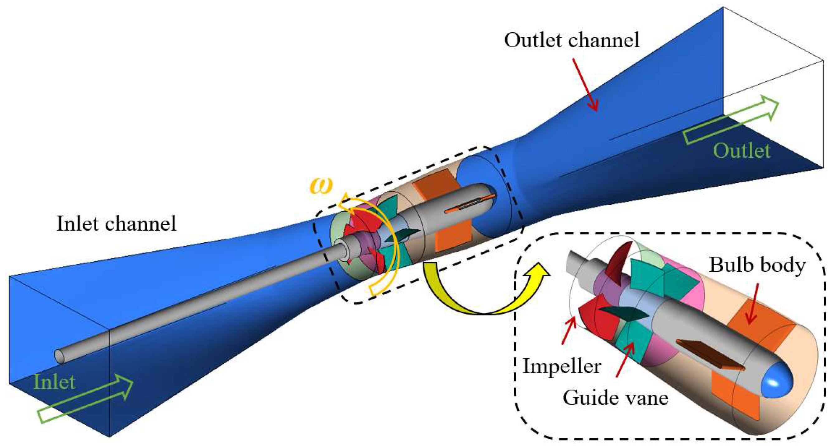
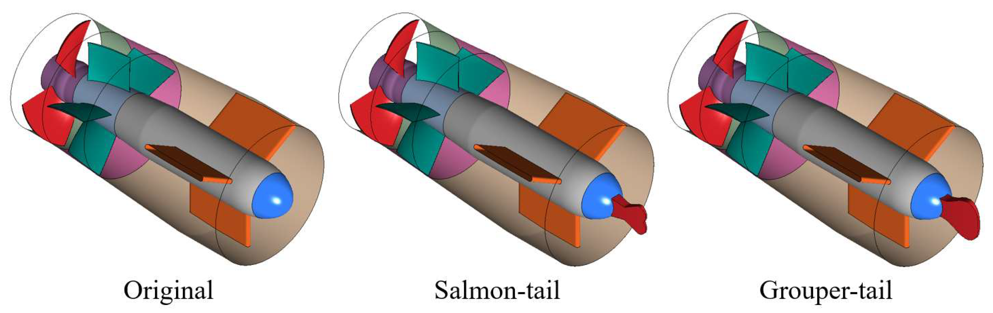
Figure 1 shows the three-dimensional model of the bulb tubular pump. Based on NX12, the water body model was established. The computational domain consists of the inlet conduit, impeller, guide vanes, bulb body, and outlet channel. The inlet and outlet channels were designed to ensure sufficiently developed flow at the inlet and outlet of the pump system. The impeller serves as the primary energy conversion component, while the guide vanes recover part of the kinetic energy at the impeller outlet and improve the downstream flow conditions. The bulb body is located at the center of the flow passage, accommodates the drive components, and significantly influences the flow-field distribution downstream of the guide vanes.

The model pump has three impeller blades, five guide vanes, and three bulb body support struts. The impeller diameter is 120 mm, and the blade-tip clearance is 0.1 mm. The pump operates at a rotational speed of 2000 r/min, with a design flow rate $Q_{des}$ of 30 L/s and a design head of 1 m.

2.2. Design of Bionic Fish-Tail Bulb Bodies

The rear geometry of the bulb body strongly influences flow reorganization between the guide-vane outlet and the outlet channel. Under off-design conditions, the interaction between the nonuniform guide-vane outflow, residual swirl, and passage diffusion can promote flow separation, recirculation, and wake development, thereby increasing local energy dissipation and pressure fluctuations. Therefore, modifying the rear geometry of the bulb body provides a potential means of regulating the downstream wake.

Inspired by the characteristic morphology of fish tails, including caudal-peduncle contraction, tail widening, and trailing-edge shape [30,31,32,33,34,35,36], static fish-tail geometries were introduced into the rear of the bulb body for passive wake control. The design focuses on geometric effects rather than active tail oscillation.

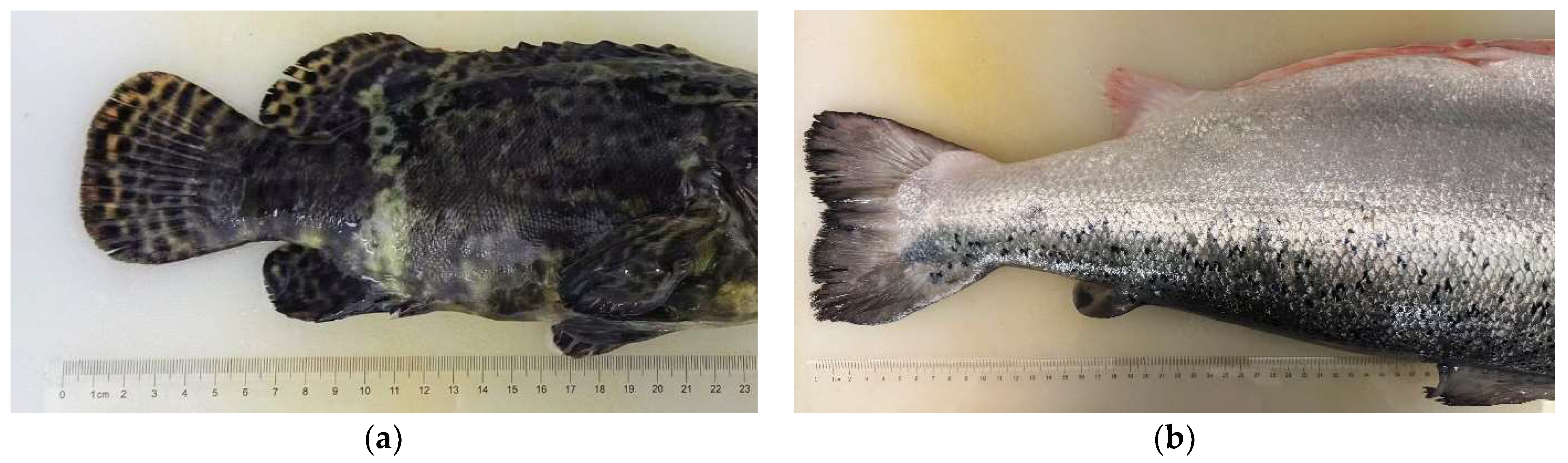
Salmon and grouper tails were selected as two geometric prototypes, as shown in Figure 2. The salmon tail features a slender caudal peduncle, pronounced axial contraction, and a forked trailing edge, whereas the grouper tail has a broader profile, shorter contraction region, and more rounded trailing edge. These morphological differences provide two distinct rear-geometry strategies. Their outer contours were subsequently extracted, nondimensionalized, and mapped onto the rear of the bulb body to construct the corresponding three-dimensional bionic geometries.

2.2.1. Fish-Tail Image Preprocessing and Extraction-Region Definition

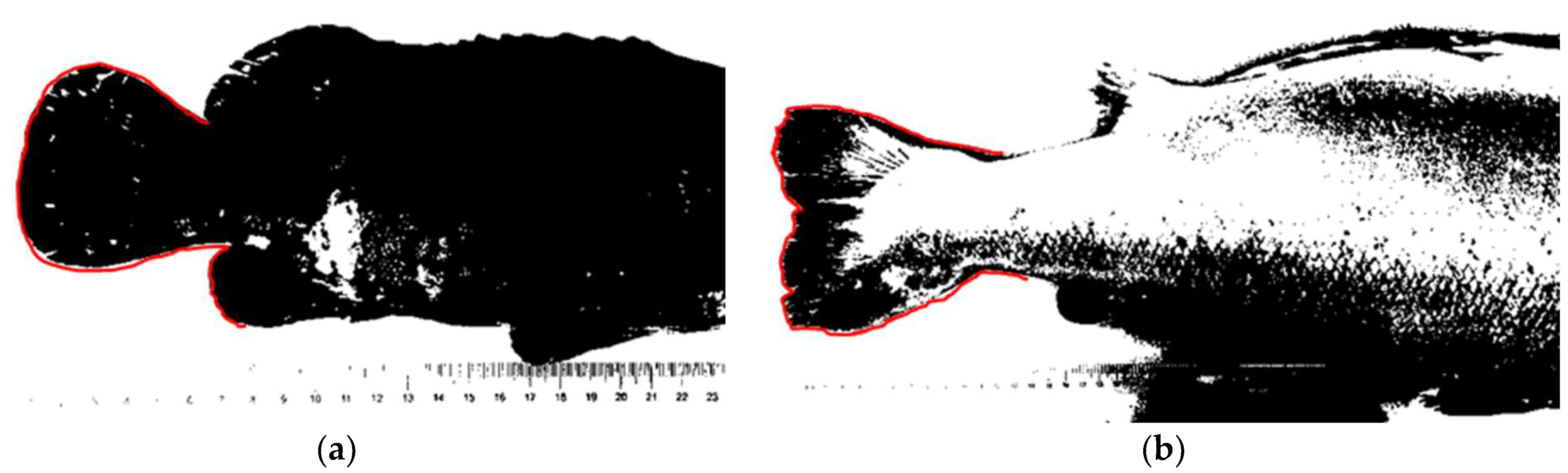
The black-and-white fish-tail images shown in Figure 3 were used to extract the macroscopic outer envelopes of the tails rather than to reconstruct their morphology at the pixel level. The effective geometric extraction region was first defined using the red boundary, while the principal morphological features, including the distal trailing edge, upper and lower outer contours, and caudal-peduncle transition region, were retained. Details irrelevant to the engineering geometry, such as local texture holes, serrations associated with fin rays, and scale markings, were removed. This procedure yielded simplified fish-tail profiles suitable for the bionic design of the rear of the bulb body.

During contour processing, the macroscopic geometric features to be retained were first identified from the original fish-tail images, and the corresponding outer envelopes were obtained from the prescribed extraction boundaries. The extracted envelopes were then represented by continuous smooth control curves, followed by nondimensionalization and piecewise-function fitting to determine the characteristic parameters and fitting coefficients listed in

Table 1. Characteristic parameters of the piecewise-fitted fish-tail outer envelopes.

Fishtail	${\mathit{L}}_{\mathit{b}}$/D	${\mathit{R}}_{\mathit{b}}$/D	$\mathit{F}\left(0\right)$	${\mathit{X}}_{\mathit{n}}$	$\mathit{F}\left({\mathit{X}}_{\mathit{n}}\right)$	${\mathit{X}}_{\mathit{m}}$	$\mathit{\lambda }$	${\mathit{R}}^2$
Salmon tail	0.25	0.43	0.6111	0.3521	0.4630	0.8028	0.6481	0.9964
Grouper tail	0.22	0.45	0.4545	0.0845	0.4545	0.7324	0.3182	0.9963

and

Table 2. Coefficients of the piecewise cubic functions for the fish-tail outer envelopes.

Fish-Tail	Segment Interval	${\mathit{c}}_0$	${\mathit{c}}_1$	${\mathit{c}}_2$	${\mathit{c}}_3$
Salmon tail	$0\le X\le X_n$	0.611111	−0.062319	−0.236580	0.150751
Salmon tail	$X_n<X\le X_m$	0.462963	0.252608	0.763476	−0.479047
Salmon tail	$X_m<X\le 1$	1.000000	0.022288	−0.251506	−0.122634
Grouper tail	$0\le X\le X_n$	0.454545	0.000000	0.000000	0.000000
Grouper tail	$X_n<X\le X_m$	0.454545	0.242105	1.167776	−0.864426

. Finally, the nondimensional control curves were mapped onto the design region at the rear of the bulb body to determine the dimensional geometric parameters required for constructing the three-dimensional bionic models.

2.2.2. Parameterization and Geometric Mapping of the Fish-Tail Outer Envelope

To ensure that the bionic bulb body geometries were derived from the actual fish-tail morphology, the white tail profiles within the prescribed regions were used for geometric extraction. The original images were first converted to grayscale, and the red calibration boundaries were used to define the geometric extraction regions. The upper and lower outer boundaries of the white region were then extracted. Let the upper and lower boundaries be denoted by $y_u\left(x\right)$ and $y_l\left(x\right)$, respectively. The local half-width of the fish tail is defined as:

$$h(x)={\displaystyle \frac{\left[y_l\right(x)-y_u(x\left)\right]}{2}}$$

(1)

where $x$ denotes the axial coordinate along the fish tail. To eliminate the influence of image size on the extracted geometric parameters, the initial and terminal sections of the calibrated region were defined as $x_0$ and $x_e$, respectively. The nondimensional axial coordinate $X$ and normalized half-width function $F\left(X\right)$ were then defined as:

$$X={\displaystyle \frac{x-x_0}{x_e-x_0}},F(X)={\displaystyle \frac{h\left(x\right)}{h_{max}}}$$

(2)

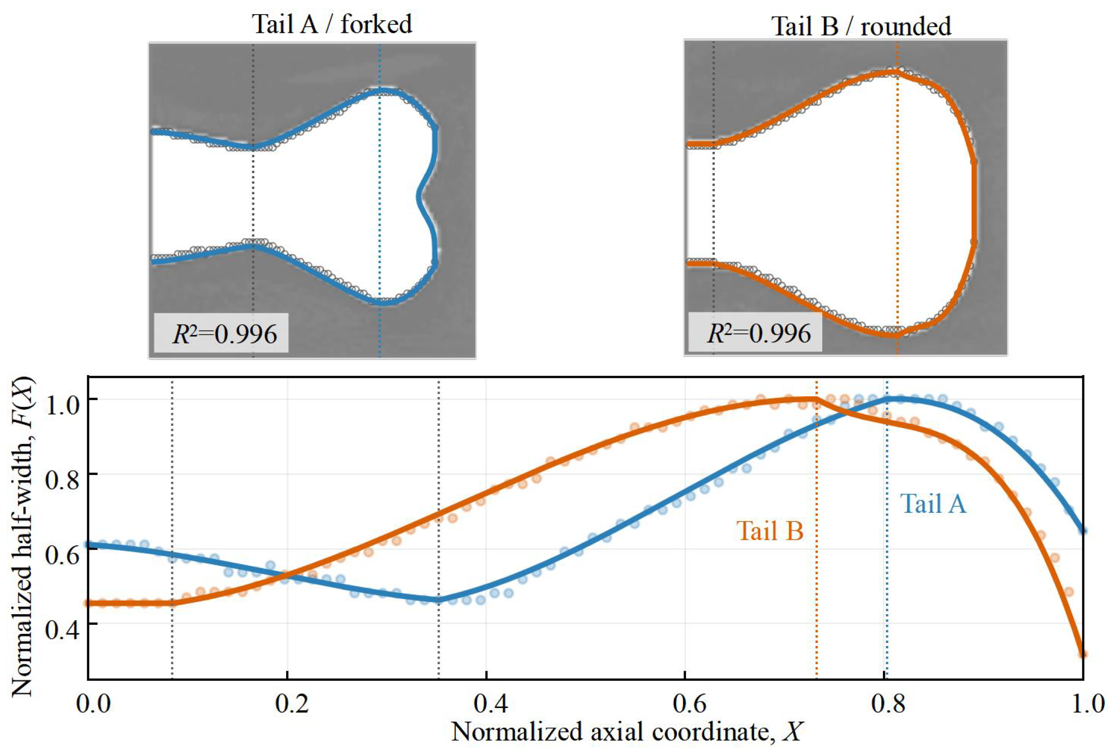
where $h_{max}$ is the maximum half-width of the extracted outer envelope. Because the fish-tail profile exhibits a nonmonotonic variation along the axial direction, including contraction near the connection region, subsequent widening of the caudal-fin region, and recovery toward the trailing edge, a single polynomial cannot adequately represent all geometric features. Therefore, the outer envelope was fitted using three piecewise cubic polynomials, as shown in Figure 4.

The piecewise cubic function is expressed as:

$$F(X)=\left\{\begin{array}{c}{c}_{10}+c_{11}{t}_1+c_{12}{t_1}^2+c_{13}{t_1}^3,0\le X\le X_n\\ c_{20}+c_{21}{t}_2+c_{22}{t_2}^2+c_{23}{t_2}^3,X_n<X\le X_m\\ c_{30}+c_{31}{t}_3+c_{32}{t_3}^2+c_{33}{t_3}^3,X_m<X\le 1\end{array}\right.$$

(3)

where $X_n$ denotes the end of the contraction region and $X_m$ denotes the axial position of maximum widening. The local coordinates are defined as:

$$t_1={\displaystyle \frac{X}{X_n}},t_2={\displaystyle \frac{X-X_n}{X_m-X_n}},t_3={\displaystyle \frac{X-X_m}{1-X_m}}$$

(4)

The trailing-edge contraction ratio is defined as:

$$\lambda =F\left(1\right)$$

(5)

The characteristic parameters obtained for the salmon and grouper tails are summarized in Table 1. The coefficient of determination $R^2$ exceeds 0.996 for both profiles, indicating that the piecewise cubic representation accurately captures the overall geometric characteristics of the extracted fish-tail envelopes.

The salmon tail exhibits a pronounced forked trailing edge. A straight-line closure would therefore suppress the characteristic central concavity of the original morphology. Accordingly, its trailing edge was represented using the following parametric curve:

$$X_c\left(\eta \right)=1-{\delta }_A{(1-{\eta }^2)}^{p_A},Y_c\left(\eta \right)={\lambda }_A\eta ,-1\le \eta \le 1$$

(6)

where ${\delta }_A=0.0581$, $p_A=7.40$, and ${\lambda }_A=0.6481$. The curve connects continuously with the upper and lower outer envelopes at its two endpoints while retaining the inward concavity at the center of the forked trailing edge.

$$X_c=1,-{\lambda }_B\le Y_c\le {\lambda }_B$$

(7)

Therefore, the two-dimensional fish-tail profile is jointly composed of the upper outer envelope, the right-end closing boundary, and the lower outer envelope. The fitting coefficients of the segmented functions are shown in Table 2.

After the normalized control function $F\left(X\right)$ was obtained, it was mapped onto the design region at the rear of the bulb body. Let $L_b$ denote the axial length of the bionic modification and $R_b$ the maximum transverse half-width. The lateral boundary of the bionic rear geometry can then be expressed as:

$$z(x)=\pm R_{b}F({\displaystyle \frac{x}{L_b}}),0\le x\le L_b$$

(8)

Because $F\left(X\right)$ is normalized by the maximum half-width, $R_b$ directly represents the maximum dimensional half-width of the bionic geometry. This mapping maintains consistency among the fitted profile, the position of maximum widening, the trailing-edge contraction ratio, and the corresponding CAD dimensions, thereby avoiding geometric inconsistencies that may arise from direct fitting with a single high-order polynomial. The resulting salmon-tail geometry retains the contraction near the connection region, subsequent tail widening, and the concave forked trailing edge, whereas the grouper-tail geometry is characterized by a smoother upstream transition, a broader intermediate region, and a more rapid contraction toward the trailing edge.

Based on the above parameterization and geometric-mapping procedures, three computational configurations were established: the original bulb body, the salmon-tail bulb body, and the grouper-tail bulb body, as shown in Figure 5. Except for the rear geometry of the bulb body, the principal hydraulic components and computational-domain parameters were kept identical among the three configurations to ensure a consistent comparison. Numerical simulations were subsequently performed for all three configurations under the same operating conditions, while experimental data for the original configuration were used to validate the numerical method. The effects of the bionic geometries are subsequently evaluated in terms of hydraulic performance, wake-flow characteristics, vortex evolution, entropy production losses, and pressure pulsations.

2.3. Numerical Method

2.3.1. Governing Equations and Turbulence Model

The working fluid in the bulb tubular pump was assumed to be incompressible, and the heat-transfer effects were neglected. The three-dimensional incompressible Reynolds-averaged Navier–Stokes (RANS) equations were solved to describe the internal flow. The continuity and momentum equations are expressed as:

$${\displaystyle \frac{\partial \overline{u_i}}{\partial x_i}}=0$$

(9)

$${\displaystyle \frac{\partial \overline{u_i}}{\partial t}}+{\displaystyle \frac{\partial \left(\overline{u_i}\overline{u_j}\right)}{\partial x_j}}=-{\displaystyle \frac{1}{\rho }}{\displaystyle \frac{\partial \overline{p}}{\partial x_i}}+{\displaystyle \frac{\partial }{\partial x_j}}\left[\upsilon \left({\displaystyle \frac{\partial \overline{u_i}}{\partial x_j}}+{\displaystyle \frac{\partial \overline{u_j}}{\partial x_i}}\right)\right]-{\displaystyle \frac{\partial \left(\overline{u_i^{\prime }{u}_j^{\prime }}\right)}{\partial x_j}}+f_i$$

(10)

Here, $u_i$ denotes the velocity component in the $x_i$ direction; $t$ is time; $\rho$ is the fluid density; $p$ is the static pressure; $\upsilon$ is the kinematic viscosity; $\overline{\varphi }$ and ${\varphi }^{\prime }$ denote the time-averaged and fluctuating components, respectively; and $f_i$ represents the body-force term.

To improve the prediction of complex rotational and curved flows in the impeller and downstream regions, the SST k-ω model with rotation–curvature correction (SST-CC) was employed. The correction accounts for the effects of streamline curvature and system rotation on turbulence production and thereby improves the applicability of the SST model to rotating flows. The original SST model was developed by Menter [39], while the rotation–curvature correction was introduced by Spalart and Shur [40] and subsequently incorporated into the SST framework by Smirnov and Menter [41]. Its application to rotating impeller flows has also been reported in Ref. [42].

The transport equations for the turbulent kinetic energy k and specific dissipation rate ω are written as:

$${\displaystyle \frac{\partial k}{\partial t}}+{\displaystyle \frac{\partial \left(\overline{u_j}k\right)}{\partial x_j}}={\displaystyle \frac{\partial }{\partial x_j}}\left[\left(\upsilon +{\upsilon }_t{\sigma }_k\right){\displaystyle \frac{\partial k}{\partial x_j}}\right]+f_{r1}{P}_k-{\beta }^{\prime }k\omega$$

(11)

$${\displaystyle \frac{\partial \omega }{\partial t}}+{\displaystyle \frac{\partial \left(\overline{u_j}\omega \right)}{\partial x_j}}={\displaystyle \frac{\partial }{\partial x_j}}\left[\left(\upsilon +{\upsilon }_t{\sigma }_{\omega }\right){\displaystyle \frac{\partial \omega }{\partial x_j}}\right]+2\left(1-F_1\right){\displaystyle \frac{{\sigma }_{\omega 2}}{\omega }}{\displaystyle \frac{\partial k}{\partial x_j}}{\displaystyle \frac{\partial \omega }{\partial x_j}}+{\alpha f}_{r1}{\displaystyle \frac{\omega }{k}}{P}_k-\beta {\omega }^2$$

(12)

where ${\upsilon }_t$ is the eddy viscosity, $P_k$ is the turbulent kinetic-energy production term, $F_1$ is the blending function, and $f_{r1}$ is the rotation–curvature correction coefficient. The model constants are ${\beta }^{\prime }=0.09$, ${\sigma }_{k1}=0.85$, ${\sigma }_{k2}=1$, ${\sigma }_{\omega 1}=0.5$, ${\sigma }_{\omega 2}=0.856$, ${\alpha }_1=5/9$, ${\alpha }_2=0.44$, ${\beta }_1=0.075$, and ${\beta }_2=0.0828$, with the corresponding coefficients blended using $F_1$.

The rotation-correction coefficient $f_{r1}$ is defined as follows:

$$f_{r1}=\mathrm{m}\mathrm{a}\mathrm{x}\left\{\mathrm{m}\mathrm{i}\mathrm{n}\left(f_r,1.25\right),0\right\}$$

(13)

$$f_r=\left(1+c_{r1}\right){\displaystyle \frac{2r^{*}}{1+r^{*}}}\left[1-c_{r3}\arctan \left(c_{r2}\tilde{r}\right)-c_{r1}\right]$$

(14)

$$r^{\mathrm{*}}={\displaystyle \frac{S}{\mathsf{\Omega }}},\tilde{r}=2{\mathsf{\Omega }}_{ik}{S}_{ik}{\displaystyle \frac{D{S}_{ij}}{Dt}}{\displaystyle \frac{1}{\mathsf{\Omega }{D}^3}},{\mathsf{\Omega }}_{ij}={\displaystyle \frac{1}{2}}\left({\displaystyle \frac{\partial U_i}{\partial x_j}}-{\displaystyle \frac{\partial U_j}{\partial x_i}}\right),D^2=\mathrm{m}\mathrm{a}\mathrm{x}\left(S^2,0.09{\omega }^2\right)$$

(15)

Here, the constants are $c_{r1}=1$, $c_{r2}=2$, and $c_{r3}=1$. $D{S}_{ij}/D_t$ is the component of the Lagrangian derivative of the strain tensor.

2.3.2. Mesh Generation and Independence Analysis

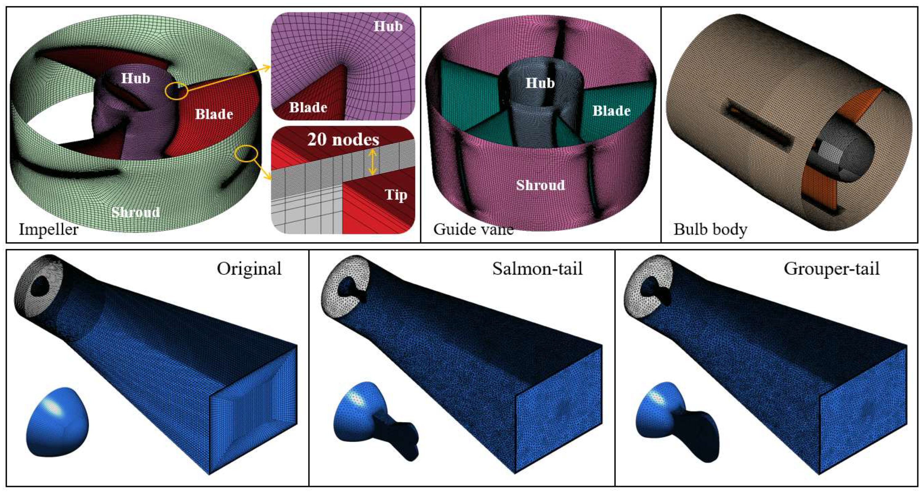
Different meshing strategies were adopted for individual computational subdomains to balance numerical accuracy and computational cost. As shown in Figure 6, structured meshes were generated for the impeller, guide-vane region, bulb body region, inlet channel, and the original outlet channel. Unstructured meshes were employed in the outlet channel regions containing the salmon-tail and grouper-tail geometries to accommodate their more complex surface shapes. Twenty grid layers were distributed across the blade-tip clearance to adequately resolve the tip-clearance flow. Boundary-layer refinement was applied to all solid walls to improve the near-wall resolution required by the SST-CC model.

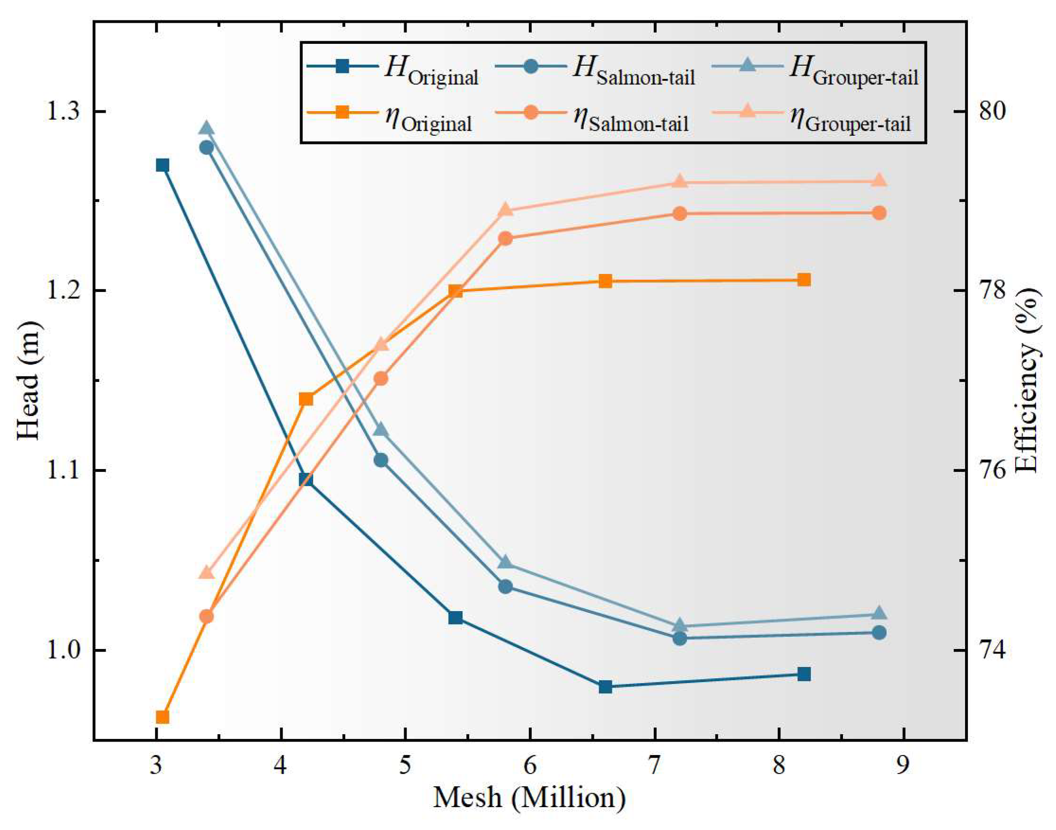
Mesh-independence analyses were conducted separately for the original, salmon-tail, and grouper-tail configurations, as shown in Figure 7. Both head and efficiency gradually approached mesh-independent values as the cell count increased. Considering the balance between numerical accuracy and computational cost, the final meshes contained approximately 6.60 million cells for the original configuration and 7.20 million cells for both the salmon-tail and grouper-tail configurations. These meshes were used for all subsequent simulations.

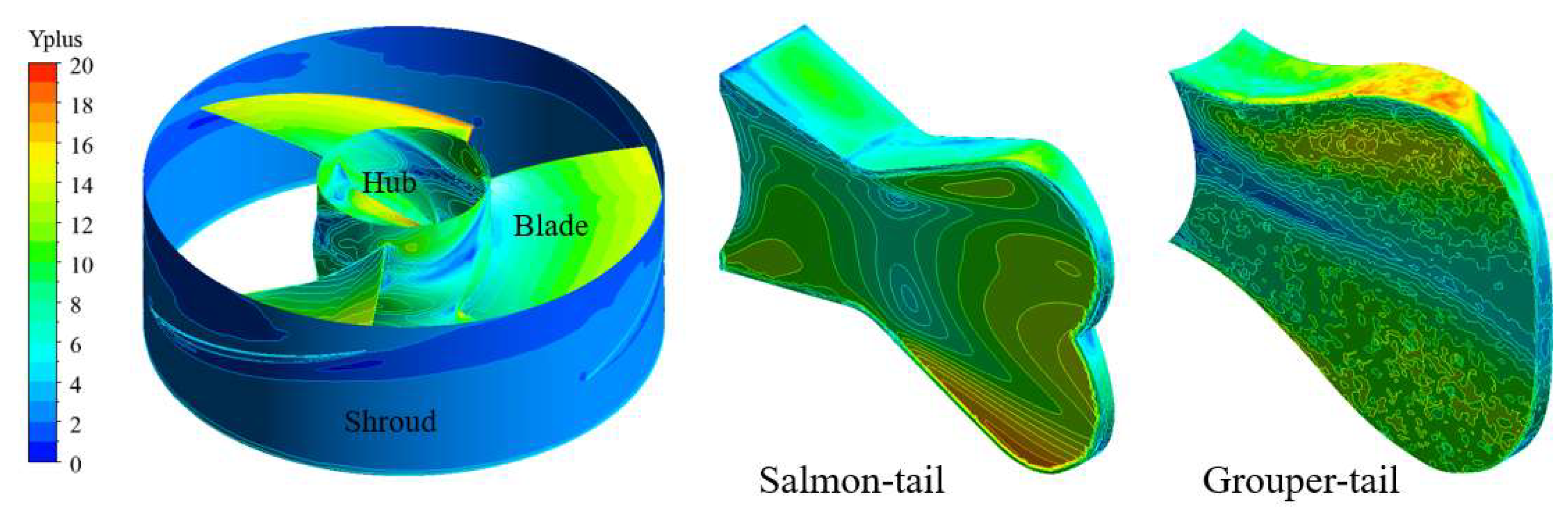
The Y+ distributions over the impeller and bionic rear surfaces obtained using the selected meshes are shown in Figure 8. The mean Y+ values on the blade, hub, and shroud surfaces were 10.29, 5.08, and 2.22, respectively, while those on the salmon-tail and grouper-tail surfaces were 8.88 and 7.85, respectively. These values indicate that the near-wall mesh resolution was compatible with the wall treatment employed by the SST-CC model and was therefore adopted for the subsequent analyses of internal flow, energy dissipation, and pressure pulsations.

2.3.3. Boundary Conditions and Solver Settings

To accurately simulate the flow characteristics of the bulb tubular pump device, the finite-volume method was used to discretize the governing equations. The computational domain included the inlet channel, impeller, guide vanes, bulb body, and outlet channel. The inlet boundary was set as a total-pressure inlet with a total pressure of 1 atm. The outlet boundary was set as a mass-flow outlet, with the flow rate specified according to the operating condition. No-slip boundary conditions were applied to all solid walls.

The impeller was defined as a rotating domain, whereas the remaining computational domains were stationary. For the steady-state simulations, the interfaces between the rotating and stationary domains were treated using the Frozen Rotor approach. The converged steady-state solution was subsequently used to initialize the transient calculation. For the transient simulations, the interfaces were treated using the Transient Rotor-Stator approach. The time step corresponded to 3 degrees of impeller rotation, and each transient simulation covered ten complete impeller revolutions to capture the unsteady flow evolution.

The diffusion terms were discretized using a central-difference scheme, while the advection terms employed the high-resolution scheme. A second-order backward Euler scheme was used for temporal discretization to maintain temporal accuracy and numerical stability.

2.4. Experimental Validation

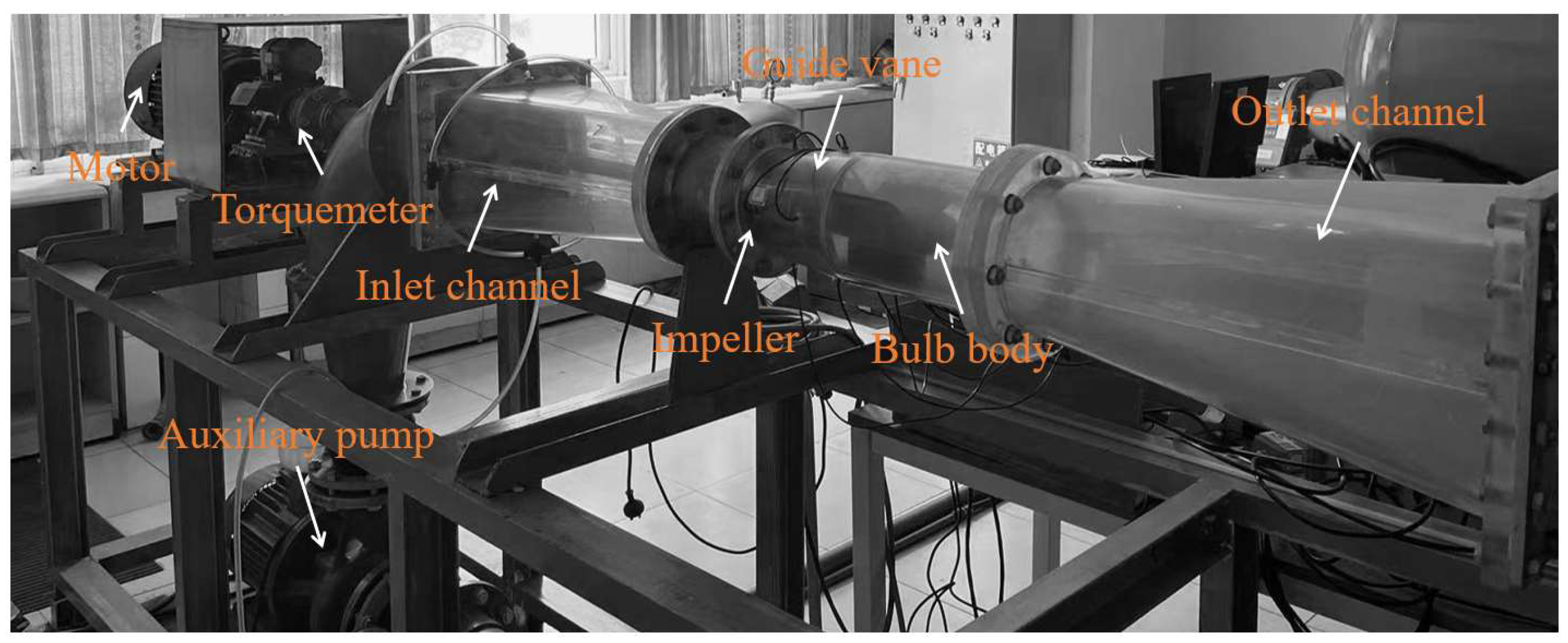
To validate the numerical method, model tests of the bulb tubular pump with the original bulb body configuration were conducted in 2025 at the Jiangsu Key Laboratory of Hydraulic Power Engineering, Yangzhou University. The experimental data used for numerical validation were collected during the same experimental campaign. The experimental setup is shown in Figure 9. The test system consisted primarily of an inlet conduit, impeller, guide vanes, bulb body, outlet channel, motor, torque and rotational-speed sensor, electromagnetic flowmeter, auxiliary pump, and associated piping system. During the experiments, the rotational speed of the model pump was maintained at 2000 r/min, while the operating flow rate was adjusted by varying the valve opening and the rotational speed of the auxiliary pump.

The principal measuring instruments included a differential-pressure transmitter, an electromagnetic flowmeter, a torque and rotational-speed sensor, and a digital torque and rotational-speed indicator. Their models, measurement ranges, and accuracies are listed in

Table 3. Main measuring instruments used in the experimental setup.

Instrument	Model	Measurement Range	Accuracy
Differential-pressure transmitter	EJA110A	0–100 kPa	0.075%
Electromagnetic flowmeter	LDZ-6	0–50 L/s	0.3%
Torque-speed sensor	ZL	0–10 N·m	0.2%
Digital torque-speed display	TS-3100B		0.05%

. Based on the systematic and random error analysis of the measurement system, the combined relative uncertainty of the pump system efficiency was ±0.479%, indicating that the experimental setup provided sufficient measurement accuracy for validating the numerical results.

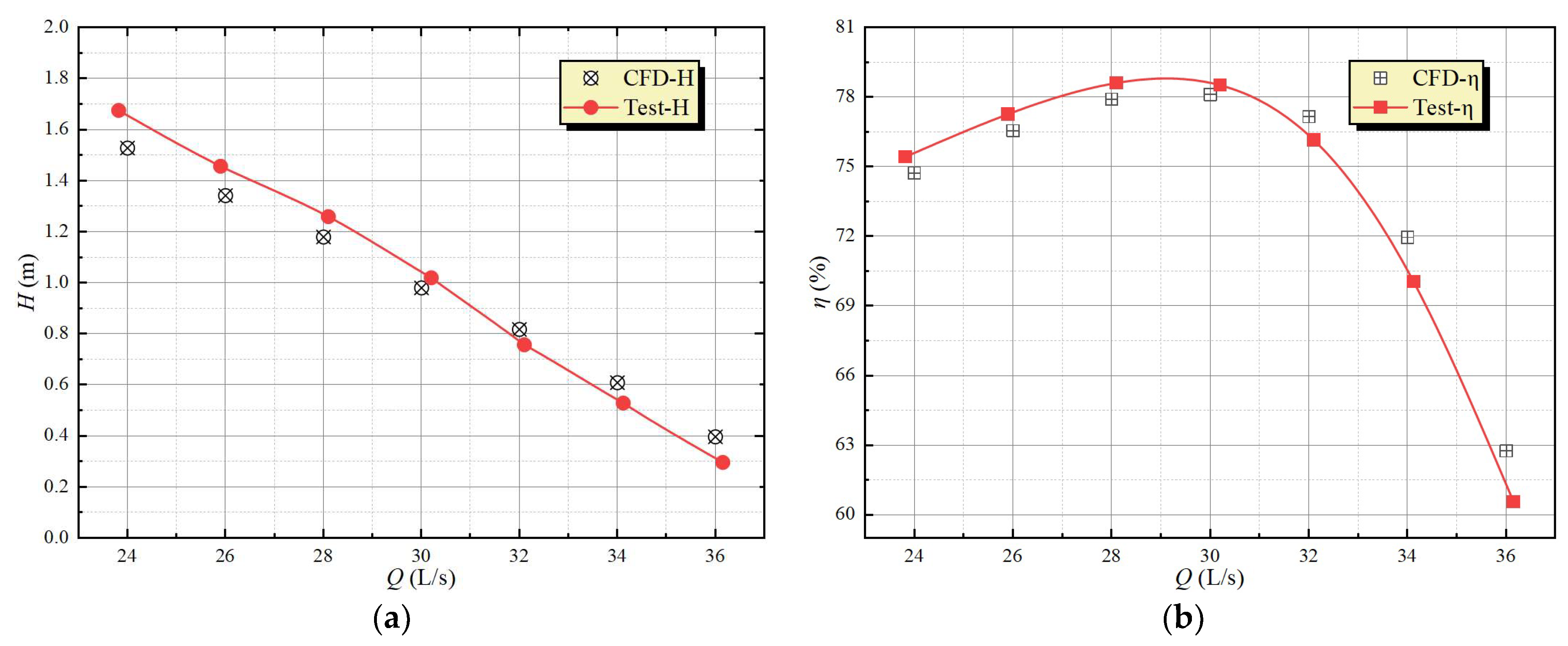
Figure 10 compares the numerically predicted and experimentally measured head and efficiency characteristics of the original configuration. The numerical results reproduce the overall trends of the experimental data. The mean relative errors of head and efficiency are 6.95% and 1.56%, respectively, while the corresponding maximum errors are 13.71% and 3.63%. The largest relative error in head occurs under the highest-flow condition, where the experimental head is relatively small, causing the relative error to be amplified. Near the design condition, the relative errors of head and efficiency are 3.92% and 0.51%, respectively. The combined relative uncertainty of the experimentally measured pump system efficiency is ±0.479%. This uncertainty characterizes the measurement system, whereas the numerical–experimental discrepancy also includes uncertainties arising from turbulence modeling, discretization, and boundary condition idealization. Overall, the quantitative comparison indicates that the adopted numerical method can reasonably reproduce the hydraulic performance characteristics of the bulb tubular pump.

It should be noted that the experimental validation in the present study was con-ducted only for the original configuration. The salmon-tail and grouper-tail configurations were evaluated numerically using the same validated computational framework. Therefore, independent experimental verification of the two bionic configurations remains a limitation of the present study and will be the focus of our subsequent work, particularly with respect to hydraulic performance and pressure-pulsation characteristics.

3. Tail-Flow Regulation Mechanism of the Bionic Fish-Tail Bulb Body

3.1. Hydraulic Performance Analysis

To quantitatively evaluate the effects of the bionic fish-tail bulb bodies on the hydraulic performance of the bulb tubular pump, the head H, efficiency $\eta$, and their relative variations were selected as performance indicators. During post-processing, $H$ and $\eta$ were calculated using the following equations:

$$H={\displaystyle \frac{P_{out}-P_{in}}{\rho g}}$$

(16)

$$\eta ={\displaystyle \frac{\rho gQH}{P_{shaft}}}\times 100\%$$

(17)

where $P$ is the total pressure at the corresponding section, $\rho$ is the fluid density, $g$ is the gravitational acceleration, $Q$ is the flow rate, and $P_{shaft}$ is the shaft input power.

To further compare the performance of the bionic configurations with that of the original configuration, the relative variations in head and efficiency, denoted by $\mathsf{\Delta }H$ and $\mathsf{\Delta }\eta$, were defined as:

$$\mathsf{\Delta }H={\displaystyle \frac{H_i-H_o}{H_o}}\times 100\%$$

(18)

$$\mathsf{\Delta }\eta ={\displaystyle \frac{{\eta }_i-{\eta }_o}{{\eta }_o}}\times 100\%$$

(19)

where the subscript $i$ denotes the bionic fish-tail configurations, including the salmon-tail and grouper-tail cases, and the subscript $o$ denotes the original configuration. A positive value of $\mathsf{\Delta }H$ or $\Delta \eta$ indicates an improvement relative to the original configuration, whereas a negative value indicates a deterioration in the corresponding performance metric.

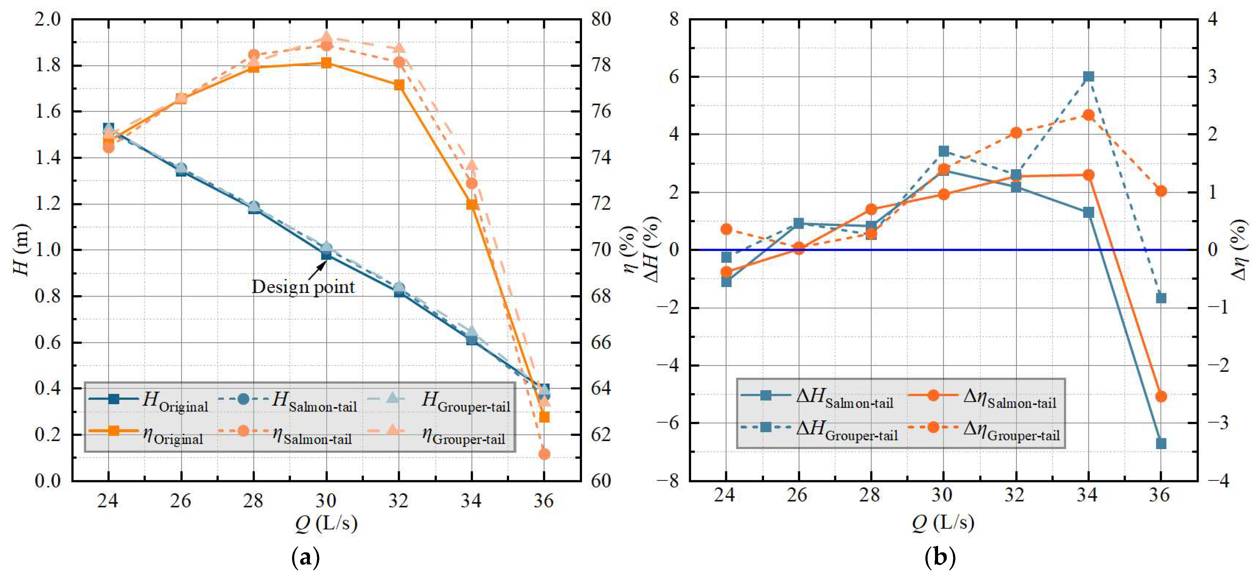
Figure 11 presents the time-averaged hydraulic performance of the bulb tubular pump under different fish-tail configurations, together with the corresponding relative variations. As shown in Figure 11a, the head decreases with increasing flow rate for all three configurations, and the corresponding curves nearly overlap, indicating that the bionic fish-tail geometries have little influence on the head characteristics. In the high-efficiency operating range, the differences in head remain small, suggesting that the bionic modifications do not introduce a noticeable head penalty. The efficiency of all three configurations first increases and then decreases with increasing flow rate, with the peak efficiency region located around Q = 30–32 L/s. Compared with the original configuration, both the salmon-tail and grouper-tail configurations exhibit efficiency improvements under most operating conditions, suggesting that the modified rear geometries can reduce hydraulic losses and improve energy conversion performance over a condition-dependent operating range.

The relative variation results in Figure 11b further show that both bionic configurations provide relatively stable positive gains over the flow rate range of Q = 28–34 L/s. The performance improvement of the salmon-tail configuration is relatively moderate, whereas the grouper-tail configuration exhibits more pronounced gains. In particular, within Q = 30–34 L/s, both $\mathsf{\Delta }H$ and $\mathsf{\Delta }\eta$ remain at comparatively high levels, indicating that the grouper-tail geometry has a stronger regulating effect on the wake flow downstream of the bulb body.

It is worth noting that, under the high-flow condition of Q = 36 L/s, the performance gains of both bionic configurations decrease markedly, and the salmon-tail configuration even exhibits reductions in both head and efficiency. This suggests that, under excessively high flow conditions, the fish-tail-inspired geometry may intensify wake-flow disturbances and thus weaken its flow-straightening and loss-reduction effects. Overall, the bionic fish-tail bulb bodies mainly improve the hydraulic performance near the design flow rate and over the medium-to-high-flow range, with the grouper-tail configuration providing greater overall performance enhancement.

3.2. Internal-Flow Characteristics

To quantitatively evaluate backflow development in the outlet channel under different flow conditions, the backflow-region volume fraction $V_C$ was introduced as an evaluation indicator. A larger $V_C$ indicates a larger backflow region and stronger flow separation. $V_C$ is calculated as follows:

$$V_{\mathrm{C}}={\displaystyle \frac{V_{rec}}{V_{out}}}\times 100\%$$

(20)

Here, $V_{rec}$ is the volume of the backflow region in the outlet channel, and $V_{out}$ is the total volume of the outlet channel.

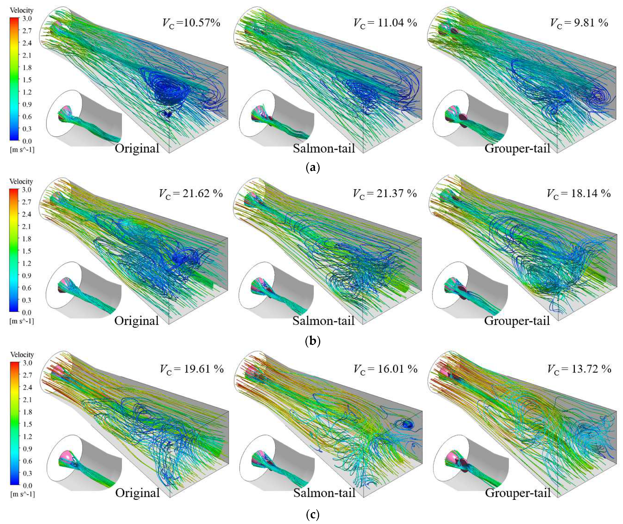
Figure 12 presents the time-averaged three-dimensional streamlines of the three configurations under representative flow conditions. At the low flow rate of Q = 24 L/s, backflow is mainly concentrated in the middle and downstream regions of the outlet channel. The backflow volume fraction $V_C$ is 10.57% for the original configuration, increases slightly to 11.04% for the salmon-tail configuration, and decreases to 9.81% for the grouper-tail configuration, indicating that the latter provides a modest suppression of backflow under the low-flow condition.

At the design flow rate of Q = 30 L/s, the backflow regions expand markedly, with $V_C$ values of 21.62%, 21.37%, and 18.14% for the original, salmon-tail, and grouper-tail configurations, respectively. Compared with the original configuration, $V_C$ decreases by only 0.25 percentage points for the salmon tail but by 3.48 percentage points for the grouper tail, demonstrating a stronger backflow-suppression effect of the latter. The results also show that the extent of backflow does not vary monotonically with flow rate but is closely related to the development of the bulb body wake and local flow separation within the outlet channel.

When the flow rate increases to Q = 36 L/s, the corresponding $V_C$ values are 19.61%, 16.01%, and 13.72%. Both bionic configurations substantially reduce the backflow region, with the grouper tail achieving the largest reduction of 5.89 percentage points relative to the original configuration. Overall, the grouper tail reduces $V_C$ under all three operating conditions, with more pronounced improvements at the design and high flow rates, whereas the salmon tail exhibits an appreciable backflow-suppression effect mainly under the high-flow condition.

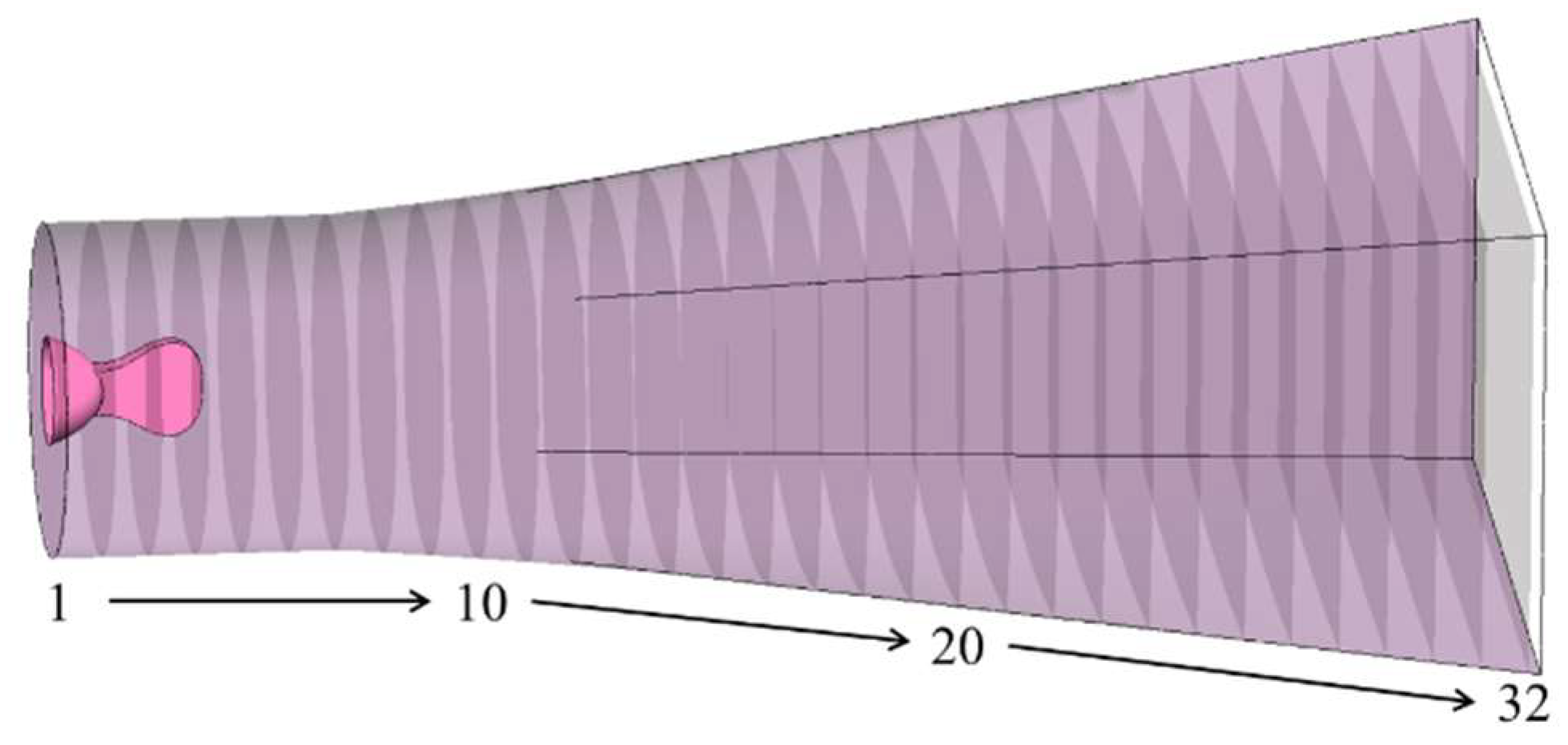
To further characterize the deviation of the local flow direction from the main flow direction, 32 equally spaced characteristic sections were arranged along the outlet channel, and the flow-deflection angle $\theta$ was evaluated at each section. As shown in Figure 13, the section numbers increase in the streamwise direction, allowing the evolution of flow deflection from the rear of the bulb body toward the outlet to be quantified. A larger $\theta$ indicates a greater deviation from the main flow direction and, consequently, poorer directional uniformity. The flow-deflection angle is defined as:

$$\theta ={\tan }^{-1}\left({\displaystyle \frac{\sqrt{v_x^2+v_z^2}}{v_y}}\right)$$

(21)

where $v_y$ is the streamwise velocity component, and $v_x$ and $v_z$ are the transverse and vertical velocity components, respectively.

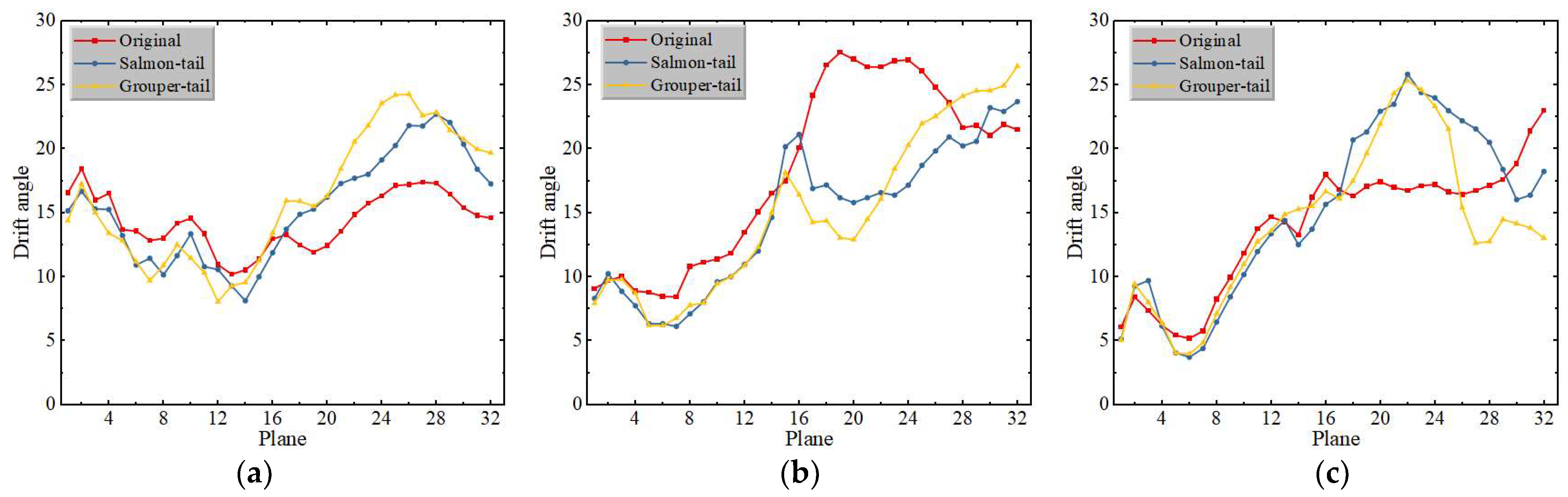
Figure 14 shows that $\theta$ varies nonuniformly along the outlet channel under all three operating conditions. Differences among the three configurations are relatively small in the upstream region, whereas flow deflection becomes more pronounced in the middle and downstream regions because of the combined effects of the bulb body wake and conduit diffusion. This indicates that the influence of the bionic fish-tail geometries on flow direction depends strongly on both axial position and operating condition rather than producing a continuous reduction in $\theta$ along the entire conduit.

At Q = 24 L/s, the two bionic configurations exhibit larger $\theta$ values than the original configuration at several downstream sections, suggesting that although the fish-tail geometries modify the extent of backflow, they also enhance local transverse velocity components. At Q = 30 L/s, the original configuration exhibits a pronounced $\theta$ peak in the middle-to-downstream region, whereas both bionic configurations reduce the flow deflection in this region; however, $\theta$ increases again near the outlet. At Q = 36 L/s, the grouper tail exhibits relatively large $\theta$ values at several intermediate sections, but shows the most pronounced decrease near the outlet, where its values become lower than those of the other two configurations.

Considering $V_C$ and $\theta$ together, the primary effect of the bionic fish-tail geometries is not to uniformly improve the flow throughout the outlet channel, but rather to modify the downstream transport and recovery of the bulb body wake. In particular, the grouper tail reduces the backflow volume fraction at the design and high flow rates and provides better flow direction recovery near the outlet under the high-flow condition, indicating a more favorable overall regulation of the outlet conduit flow.

3.3. Characteristics of Vortex Structures

Based on the preceding analyses of backflow-region scale and flow-deflection angle, the vortex-structure volume fraction $V_{\mathrm{V}}$ was introduced to further quantify the scale of vortex development in the outlet channel. It is calculated as follows:

$$V_{\mathrm{V}}={\displaystyle \frac{V_{vor}}{V_{out}}}\times 100\%$$

(22)

Here, $V_{vor}$ is the vortex-structure volume identified by the Omega method in the outlet channel. In the Omega method, a value slightly greater than 0.5 is generally used to identify regions where rotation dominates over deformation. Accordingly, a threshold of $Omega=0.53$ was adopted to distinguish coherent vortical structures from weak shear-dominated regions while retaining a clear representation of the wake-vortex structures. The same threshold was applied to all configurations and operating conditions to ensure a consistent quantitative comparison.

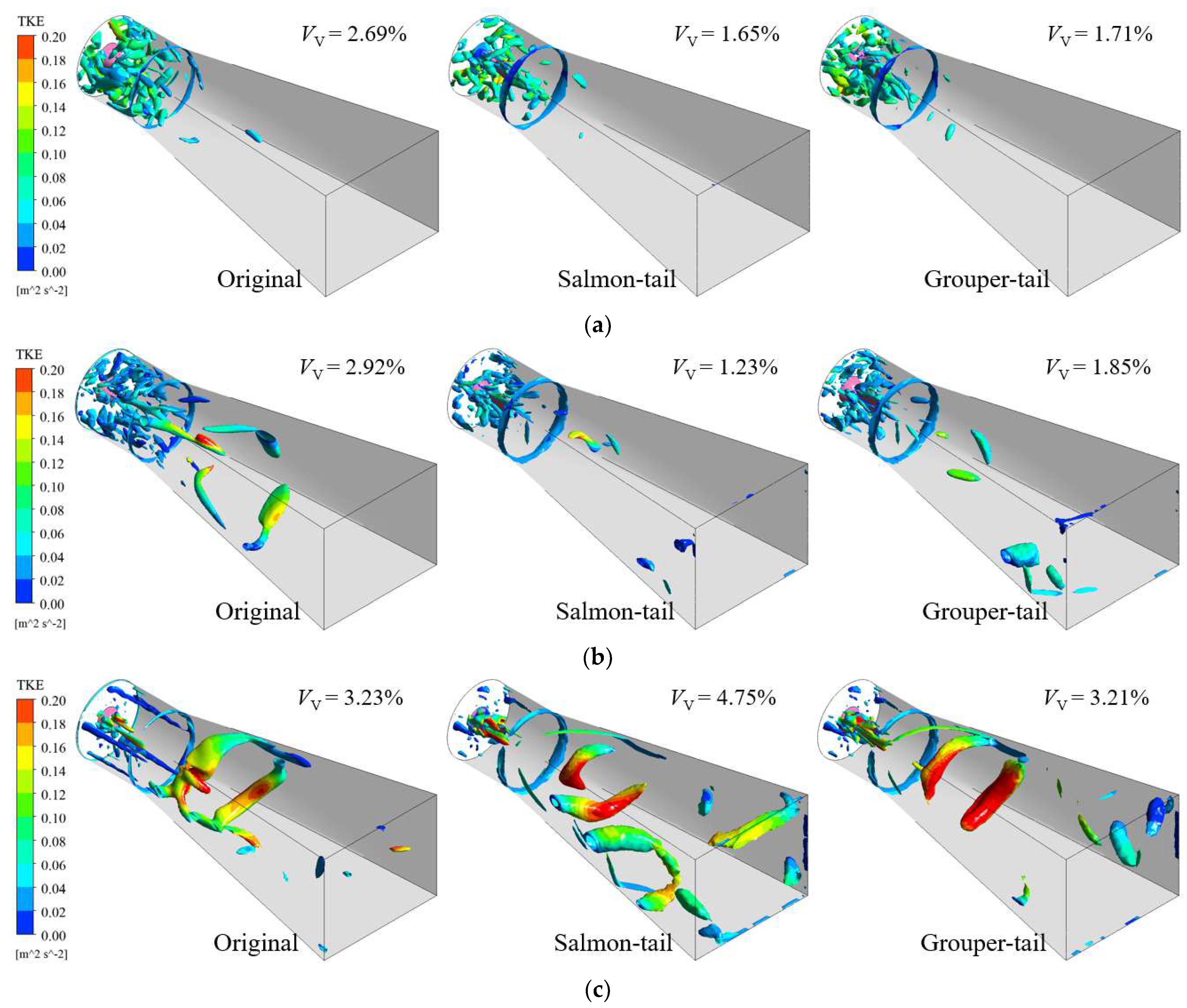
Figure 15 shows the vortex structures in the outlet channel under representative flow conditions, colored by turbulent kinetic energy. Overall, the vortices originate mainly from the bulb body wake and extend progressively toward the middle and downstream regions of the outlet channel as the flow rate increases. Their spatial distribution and intensity vary noticeably among the different fish-tail geometries.

At Q = 24 L/s, the vortex structures are concentrated near the inlet of the outlet channel, with only a few isolated vortices farther downstream. The vortex volume fraction $V_{\mathrm{V}}$ is 2.69% for the original configuration, but decreases to 1.65% and 1.71% for the salmon-tail and grouper-tail configurations, respectively, indicating that both bionic geometries effectively suppress wake-vortex development under the low-flow condition. Combined with the previous $V_C$ results, the salmon tail reduces the vortex scale without a corresponding reduction in backflow volume, whereas the grouper tail simultaneously decreases both $V_{\mathrm{V}}$ and $V_C$, indicating a more coordinated improvement in the downstream flow.

At Q = 30 L/s, $V_{\mathrm{V}}$ for the original configuration increases to 2.92%, and the vortex structures extend from the bulb body wake toward the middle of the outlet channel. The salmon-tail and grouper-tail configurations reduce $V_{\mathrm{V}}$ to 1.23% and 1.85%, respectively, demonstrating that both geometries suppress downstream wake-vortex development. The reduction is more pronounced for the salmon tail, indicating a stronger attenuation of vortex structures at the design condition.

When the flow rate increases to Q = 36 L/s, vortex shedding and downstream transport become more pronounced, and vortical structures with high turbulent kinetic energy extend farther into the middle and downstream regions of the outlet channel. The $V_{\mathrm{V}}$ values are 3.23%, 4.75%, and 3.21% for the original, salmon-tail, and grouper-tail configurations, respectively. The increase in $V_{\mathrm{V}}$ for the salmon tail indicates enhanced vortex development under the high-flow condition, consistent with its reduced gains in head and efficiency discussed above. In contrast, the grouper tail maintains a vortex level close to that of the original configuration. Together with the $V_C$ and $\theta$ results, this suggests that the grouper tail provides more stable overall regulation of wake transport, backflow, and flow direction recovery under high-flow conditions.

The preceding vortex structure analysis shows that the bionic fish-tail geometries alter the development of vortical structures in the outlet channel. To further quantify the strength and direction of residual swirl, the circulation was evaluated on cross sections distributed along the outlet channel. The section normal was defined in the Y-direction. Viewed in the downstream direction, circulation in the same direction as the counterclockwise impeller rotation was defined as positive, whereas circulation in the opposite direction was defined as negative. A larger absolute circulation indicates stronger residual swirl and, consequently, greater flow deflection and potential energy dissipation.

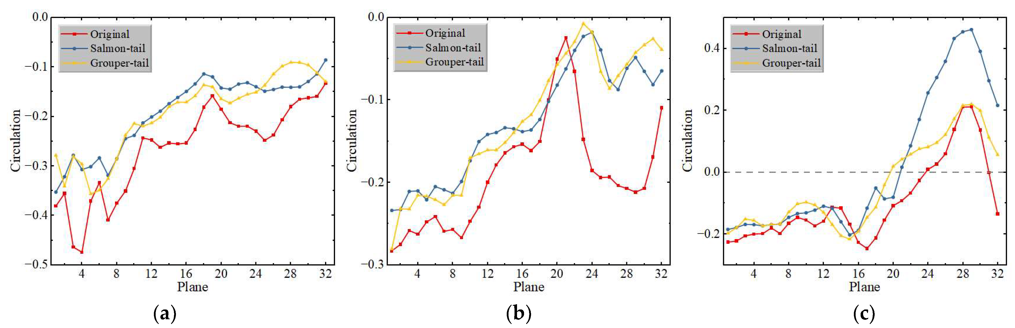
Figure 16 shows the streamwise circulation distributions of the three configurations under representative operating conditions. In general, circulation varies nonmonotonically along the outlet channel, indicating continuous redistribution of residual swirl during downstream development. As the flow rate increases, the circulation shifts from predominantly negative values at a low flow rate to values close to zero at the design condition and predominantly positive values at a high flow rate, demonstrating a strong dependence of swirl direction and intensity on the operating condition.

Under the low-flow condition of Q = 24 L/s, circulation is negative for all three configurations, indicating that residual swirl opposite to the impeller rotation direction mainly exists in the outlet channel. During downstream development, the circulation generally approaches zero, indicating gradual decay of reverse swirl. Compared with the original configuration, the two bionic fish-tail configurations have smaller absolute circulation values at most sections, indicating that the fish-tail structure can weaken reverse swirl to some extent under low-flow conditions. The salmon tail produces the smallest residual circulation near the outlet.

Under the design flow condition of Q = 30 L/s, the front sections of all three configurations still show mainly negative circulation, but the values gradually approach zero along the conduit. The original configuration shows obvious fluctuations in the middle and rear sections and returns to a relatively large negative circulation after the peak, indicating unstable recovery of residual swirl. The two bionic fish-tail configurations are generally closer to zero, especially the grouper tail, which has smaller circulation in the outlet section, indicating that it helps reduce outlet residual swirl at the design flow rate.

Under the high-flow condition of Q = 36 L/s, circulation gradually changes from negative values in the front section to positive values, indicating the formation of residual swirl in the same direction as the impeller rotation in the middle and rear regions of the conduit. The circulation of the original configuration becomes negative again at the outlet, indicating unstable adjustment of outlet swirl direction. In the salmon-tail configuration, positive circulation increases markedly in the rear half and reaches the highest peak, indicating that the salmon tail strengthens co-rotating swirl under high-flow conditions, consistent with the preceding increase in vortex-structure volume fraction. Although positive circulation also appears in the grouper-tail configuration, both its peak and outlet values are lower than those of the salmon tail, indicating a weaker amplification of residual swirl under high-flow conditions.

In summary, the influence of the bionic fish-tail structure on circulation is strongly condition-dependent. Under low-flow and design flow conditions, both fish-tail structures generally weaken reverse residual swirl. Under high-flow conditions, the salmon tail strengthens co-rotating swirl, whereas the grouper tail keeps outlet circulation at a relatively low level. Combined with the results for backflow region, flow-deflection angle, and vortex structure, the grouper tail shows more stable regulation of swirl development in the outlet channel.

4. Energy-Loss Mechanisms Based on Entropy Production Analysis

To further reveal the mechanism by which the bionic fish-tail structure affects energy loss in the outlet channel, entropy production theory was introduced on the basis of the preceding flow structure analysis to quantitatively characterize irreversible energy loss in the passage. Entropy production reflects mechanical energy loss caused by viscous dissipation, turbulent fluctuation, near-wall friction, and related factors, and its spatial distribution can be used to identify the main energy dissipation regions. By comparing entropy production distributions and contribution changes among different fish-tail configurations under representative flow conditions, the mechanism by which the bionic fish-tail structure regulates tail flow and weakens local loss can be further clarified.

4.1. Entropy Production Theory

From a thermodynamic perspective, entropy production is closely related to irreversible energy dissipation in pump systems. Therefore, analysis based on the second law of thermodynamics can be used to evaluate hydraulic losses in pump systems. For incompressible single-phase flow, the flow in hydraulic machinery can be regarded as an adiabatic process, with temperature variation and heat transfer neglected. Accordingly, the transport equation for the volumetric entropy production rate per unit mass in Cartesian coordinates is shown in Equation (23).

$$\rho \left({\displaystyle \frac{\partial s}{\partial t}}+u_i{\displaystyle \frac{\partial s}{\partial x_j}}\right)=S_D^{‴}$$

(23)

Here, $s$ is the specific entropy, and $S_D^{‴}$ is the volumetric entropy production rate.

$S_D^{‴}$ can be expressed as:

$$S_D^{‴}={\displaystyle \frac{1}{T}}{m}_{ji}{\displaystyle \frac{\partial u_i}{\partial x_j}}$$

(24)

For RANS-based simulations, the entropy production rate (EPR) can be decomposed into contributions associated with the mean flow and turbulent velocity fluctuations. EPR due to the mean velocity gradients is expressed as:

$$S_{\overline{D}}^{‴}={{\displaystyle \frac{1}{T}}m}_{ji}{\displaystyle \frac{\partial \overline{u_i}}{\partial x_j}}$$

(25)

where $m_{ji}$ denotes the time-averaged viscous stress tensor:

$$m_{ji}=\mu \left({\displaystyle \frac{\partial \overline{u_i}}{\partial x_j}}+{\displaystyle \frac{\partial \overline{u_j}}{\partial x_i}}\right)-{\displaystyle \frac{2}{3}}\mu {\delta }_{ij}{\displaystyle \frac{\partial \overline{u_i}}{\partial x_i}}$$

(26)

Here, ${\delta }_{ij}$ is the Kronecker symbol, and $\mu$ is the dynamic viscosity.

For incompressible flow in the bulb tubular pump, $S_{\overline{D}}^{‴}$ can be further written as:

$$S_{\overline{D}}^{‴}={\displaystyle \frac{2\mu }{T}}\left[{\left({\displaystyle \frac{\partial \overline{u}}{\partial x}}\right)}^2+{\left({\displaystyle \frac{\partial \overline{v}}{\partial y}}\right)}^2{+\left({\displaystyle \frac{\partial \overline{w}}{\partial z}}\right)}^2\right]+{\displaystyle \frac{\mu }{T}}\left[{\left({\displaystyle \frac{\partial \overline{u}}{\partial y}}+{\displaystyle \frac{\partial \overline{v}}{\partial x}}\right)}^2+{\left({\displaystyle \frac{\partial \overline{u}}{\partial z}}+{\displaystyle \frac{\partial \overline{w}}{\partial x}}\right)}^2{+\left({\displaystyle \frac{\partial \overline{v}}{\partial z}}+{\displaystyle \frac{\partial \overline{w}}{\partial y}}\right)}^2\right]$$

(27)

Following Kock and Herwig [20,21], the EPR associated with turbulent velocity fluctuations can be approximated using the turbulence model variables k and ω:

$$S_{D^{\prime }}^{‴}=0.09{\displaystyle \frac{\rho \omega k}{T}}$$

(28)

In addition, large velocity gradients and wall shear in the near-wall region generate additional irreversible losses. Following previous entropy production formulations [20,21,22], the wall entropy production can be evaluated as:

$$S_W={\int }_A{\displaystyle \frac{{\tau }_W\cdot v}{T}}dA$$

(29)

where ${\tau }_W$ is the wall shear stress, and $v$ is the near-wall velocity vector.

Accordingly, the total power loss associated with entropy production, $P_S$, is expressed as:

$$\begin{gathered} P_{S\overline{D}}={\int }_V{S}_{\overline{D}}^{‴}dV\cdot T \\ {P}_{S{D}^{\prime }}={\int }_V{S}_{D^{\prime }}^{‴}dV\cdot T \\ {P}_{Sw}={\int }_A{\displaystyle \frac{{\tau }_W\cdot v}{T}}dA\cdot T \\ {P}_S=P_{S\overline{D}}+P_{S{D}^{\prime }}+P_{Sw} \end{gathered}$$

(30)

Here, $P_{S\overline{D}}$, $P_{S{D}^{\prime }}$, and $P_{Sw}$ denote the mean-flow viscous, turbulent, and wall-related entropy production losses, respectively. The thermodynamic temperature $T$ was set to 298.15 K.

4.2. Quantitative Analysis of Entropy Production

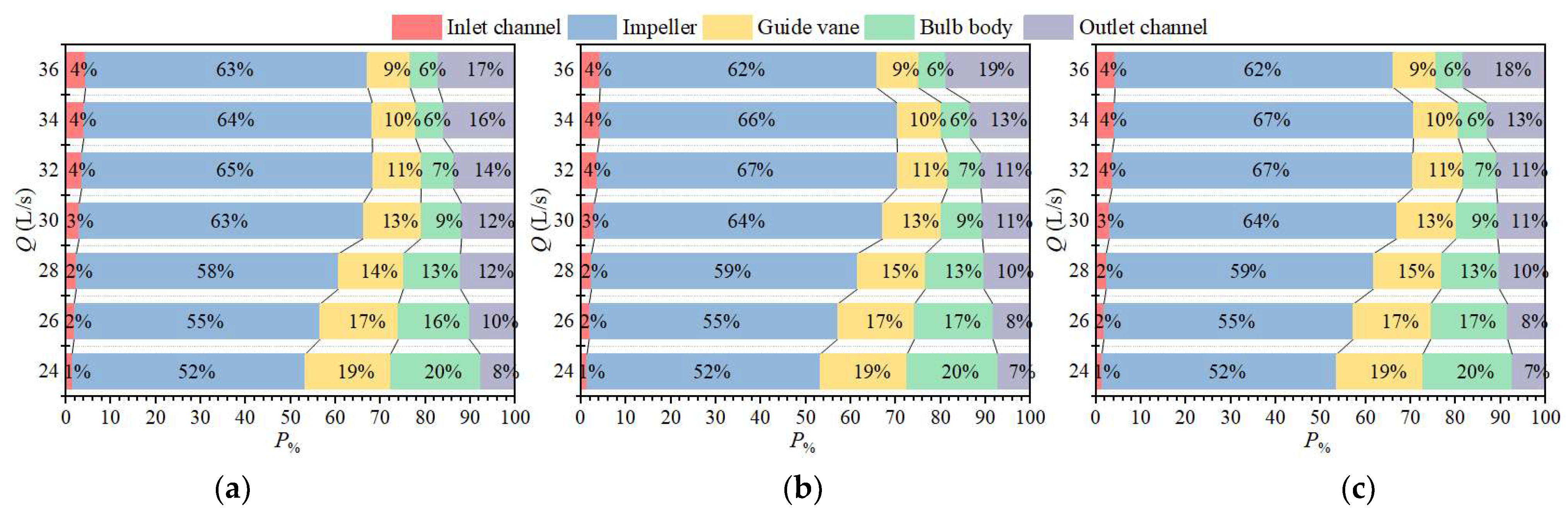
Figure 17 shows the entropy production power contributions of the main hydraulic components under different flow conditions. The three configurations exhibit similar overall distributions, with the impeller consistently accounting for the largest proportion, approximately 52–67%, indicating that irreversible energy loss is dominated by the impeller region. As the flow rate increases from 24 to 32 L/s, the impeller contribution generally increases and then decreases slightly at 36 L/s, while remaining dominant. In contrast, the contributions of the guide vanes and bulb body decrease from approximately 19% to 9% and from 20% to 6%, respectively.

The outlet channel shows the opposite trend, with its contribution increasing from approximately 7–8% at low flow rates to 17–19% at 36 L/s. This increase is associated with stronger wake transport, flow separation, and residual swirl under high-flow conditions, consistent with the preceding vortex, flow-deflection angle, and circulation analyses. Although the bionic fish-tail geometries do not alter the overall loss distribution, they modify the contribution of the outlet channel. Within Q = 24–34 L/s, the outlet channel contribution of the two bionic configurations is generally lower than or close to that of the original configuration, whereas slightly higher values occur at Q = 36 L/s. Thus, the outlet channel becomes increasingly important to the overall energy loss under high-flow conditions.

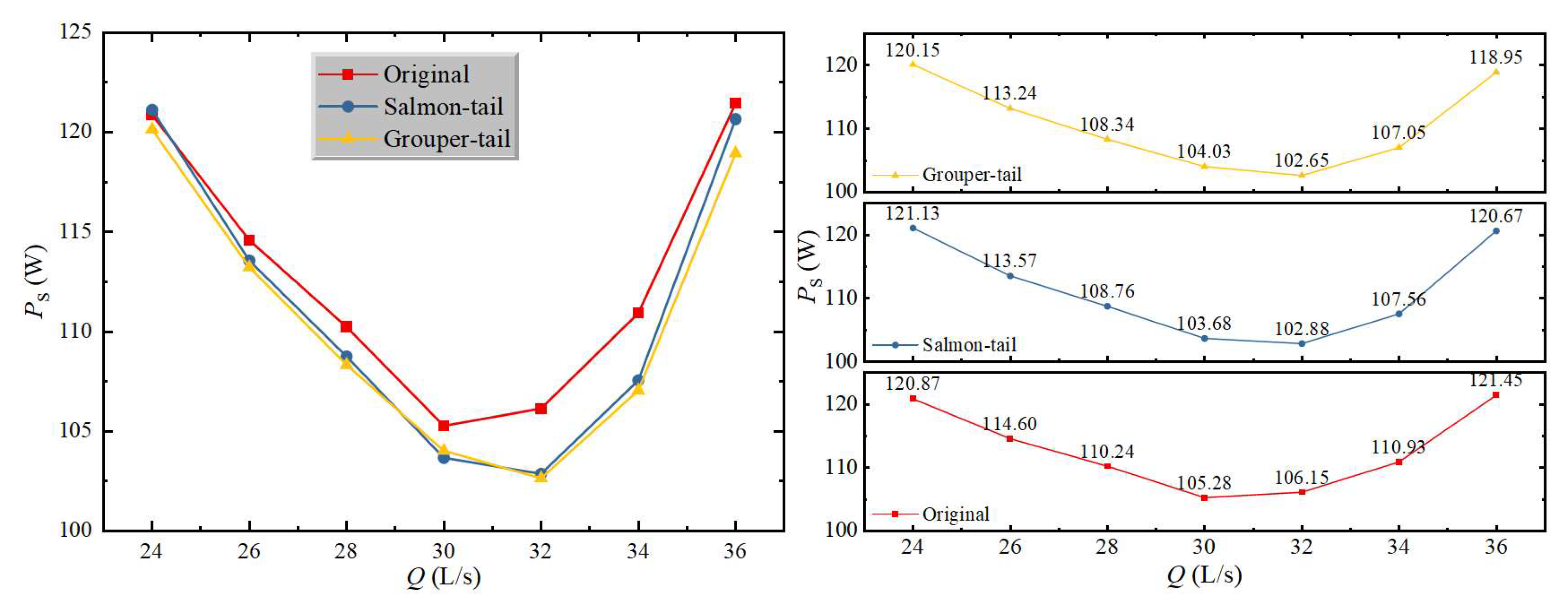
Figure 18 shows the variation in the total entropy production power $P_s$ in the outlet channel under different flow conditions. The figure shows that $P_s$ in all three configurations first decreases and then increases with increasing flow rate, giving an overall U-shaped distribution. $P_s$ is relatively low near Q = 30–32 L/s, indicating lower energy loss in the outlet channel within this flow range. Under low-flow and high-flow conditions, $P_s$ increases markedly, indicating that off-design operation intensifies irreversible energy dissipation.

Comparison among the configurations shows that $P_s$ is generally higher in the original configuration, especially under high-flow conditions, where the increase is obvious. This indicates that after the device deviates from the high-efficiency region, flow separation, vortex dissipation, and residual swirl in the outlet channel intensify, leading to increased irreversible energy loss. With the introduction of the bionic fish tail, $P_s$ is reduced under most conditions for both fish-tail configurations, except that the salmon-tail configuration is slightly higher than the original configuration at Q = 24 L/s. The grouper-tail configuration has the lowest $P_s$ at most flow rates; in particular, $P_s$ decreases to 102.65 W at Q = 32 L/s, 3.50 W lower than that of the original configuration, and to 118.95 W at Q = 36 L/s, 2.50 W lower than that of the original configuration. This indicates a more stable suppression of energy loss In the outlet channel. By contrast, the salmon-tail configuration has the lowest $P_s$ at Q = 32 L/s, 102.88 W, but shows a smaller reduction under high-flow conditions, indicating that its effect on energy-loss control is more condition-dependent.

Overall, the bionic fish-tail structure can reduce the total entropy production power of the outlet channel under most operating conditions and weaken irreversible energy loss. The grouper-tail configuration has a better overall loss-reduction effect, consistent with the preceding findings of its lower backflow-region volume fraction and better outlet flow recovery.

4.3. Qualitative Analysis of Entropy Production

On the basis of the quantitative analysis of total entropy production power in the outlet channel and of different loss sources, the EPR distribution in the outlet channel was qualitatively analyzed to further reveal the spatial distribution characteristics of energy loss. High-EPR regions indicate locations of strong local irreversible energy dissipation and are usually closely associated with flow phenomena such as flow separation, vortex-structure shedding, increased velocity gradients, and enhanced near-wall shear. Therefore, comparing the EPR distributions of different fish-tail configurations under representative flow conditions can further clarify the mechanism by which the bionic fish-tail structure regulates local loss in the outlet channel.

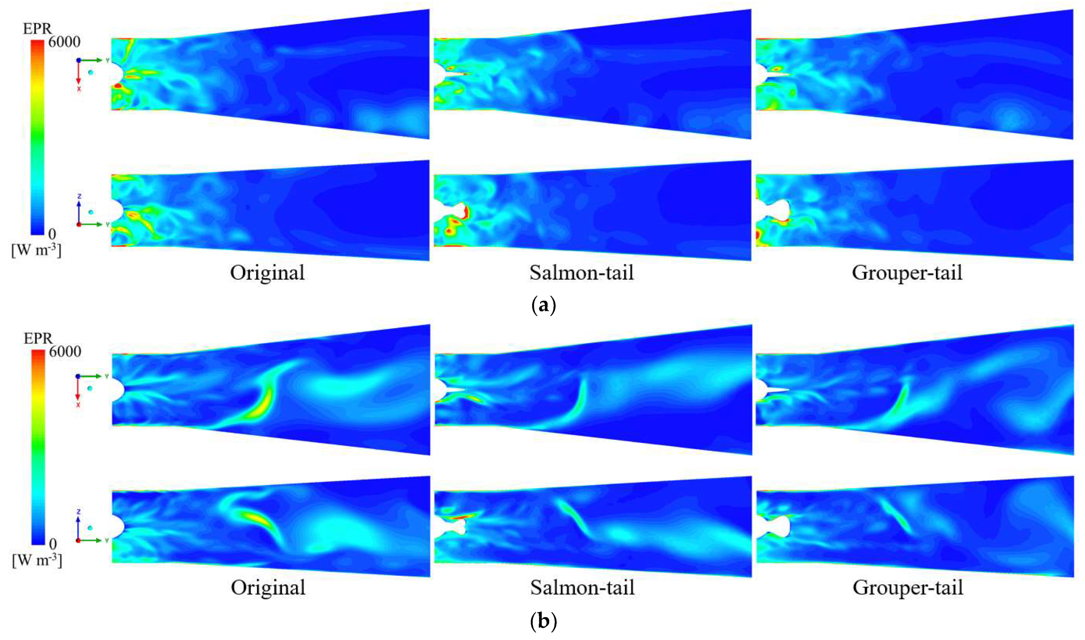
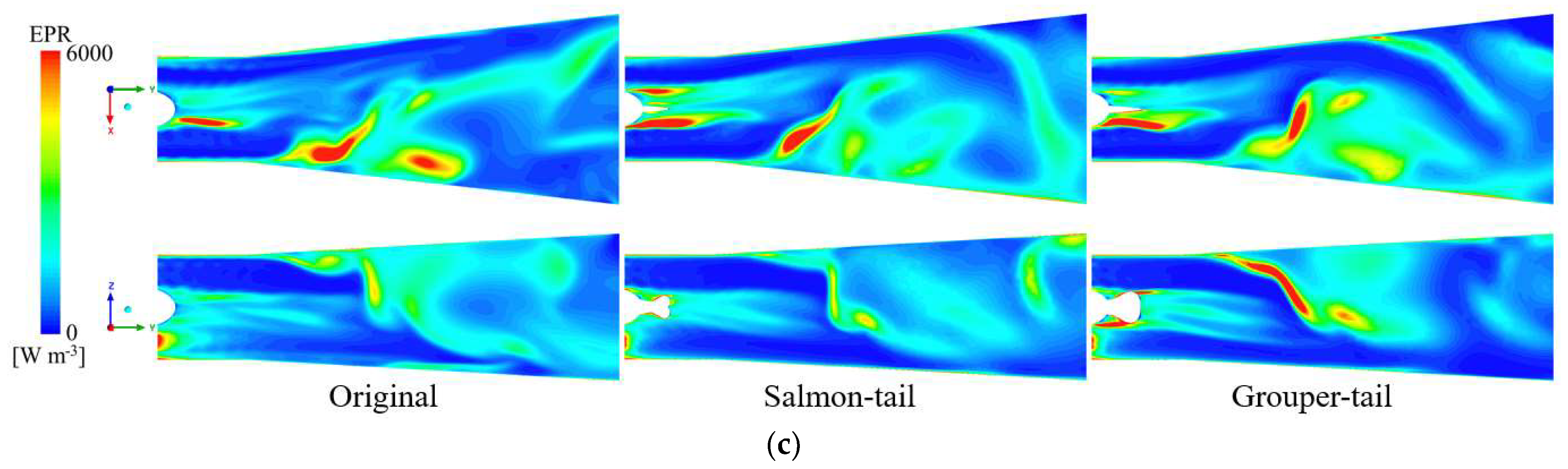
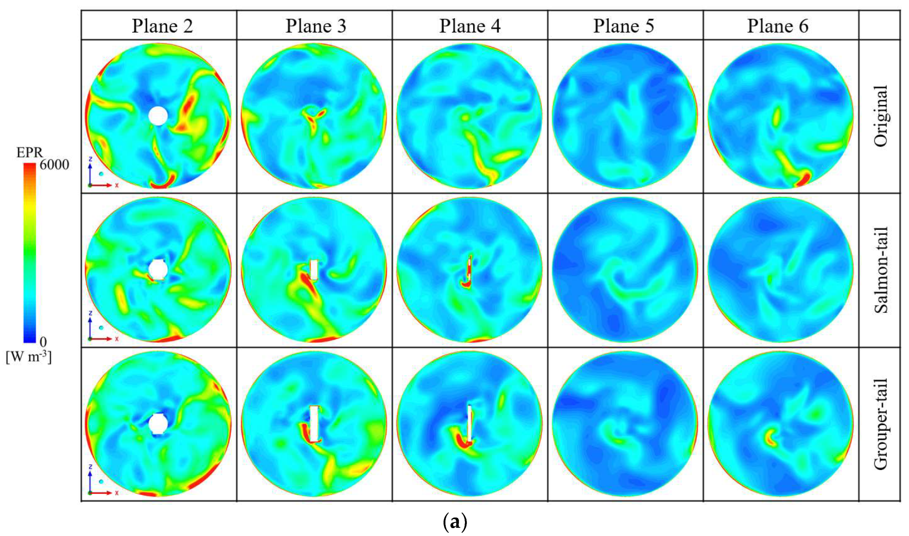
Figure 19 shows contours of the EPR on the meridional planes of the outlet channel for the three configurations under different flow conditions. In each group, the upper and lower panels correspond to the X-Y and Y-Z planes, respectively. It should be noted that the meridional plane contours represent the local EPR distribution on the middle section and are mainly used to identify local high-loss regions; their patterns may differ from the integrated entropy production results for the entire outlet channel. Therefore, the following analysis focuses on the position, range, and intensity variation of high-EPR regions.

At Q = 24 L/s, the high EPR regions of the three configurations are mainly concentrated near the rear of the bulb body and the fish-tail structure, while the overall EPR in the middle and downstream regions of the outlet channel is low. Compared with the original configuration, introducing the fish-tail structure induces new local high-EPR regions near the fish tail, indicating that fish-tail geometry enhances local shear and small-scale disturbances and therefore causes additional energy loss. The high-EPR region near the salmon tail is more obvious, indicating greater local loss under low-flow conditions.

At Q = 30 L/s, the original configuration has obvious high-EPR regions in the middle and downstream parts of the outlet channel, indicating that tail separation and downstream diffusion still cause certain energy dissipation. After the fish-tail structure is introduced, the high-EPR region in the downstream passage behind the fish tail is markedly weakened, indicating that the bionic fish tail improves wake diffusion and reduces downstream passage loss. However, a local high-EPR region appears on the left side of the salmon tail along the mainstream direction, indicating that some additional loss is still generated near the salmon tail itself. By contrast, no obvious extra high-loss region appears near the grouper tail, indicating weaker local flow disturbance at the design flow rate.

At Q = 36 L/s, high-EPR regions increase markedly in the outlet channel and are mainly distributed near and downstream of the fish tail. This indicates that stronger mainstream inertia under high-flow conditions intensifies the interaction between the fish-tail structure and the incoming flow, increasing local velocity gradients and turbulent dissipation. Both fish-tail structures induce additional flow loss near themselves, and the high-EPR region near the grouper tail is more concentrated and stronger, indicating relatively greater local additional loss under high-flow conditions.

Overall, the meridional plane EPR distributions show that the bionic fish-tail structure has a dual effect on local energy loss. On the one hand, the fish-tail structure can weaken high-EPR regions in the downstream passage at the design flow rate and improve wake diffusion. On the other hand, its own geometry can induce local additional loss near the fish tail, and this effect becomes more obvious under off-design conditions. In general, the salmon tail produces more pronounced local loss under low-flow conditions, whereas the grouper tail causes weaker local disturbance and better downstream loss control at the design flow rate but its additional loss near the fish tail increases relatively under high-flow conditions.

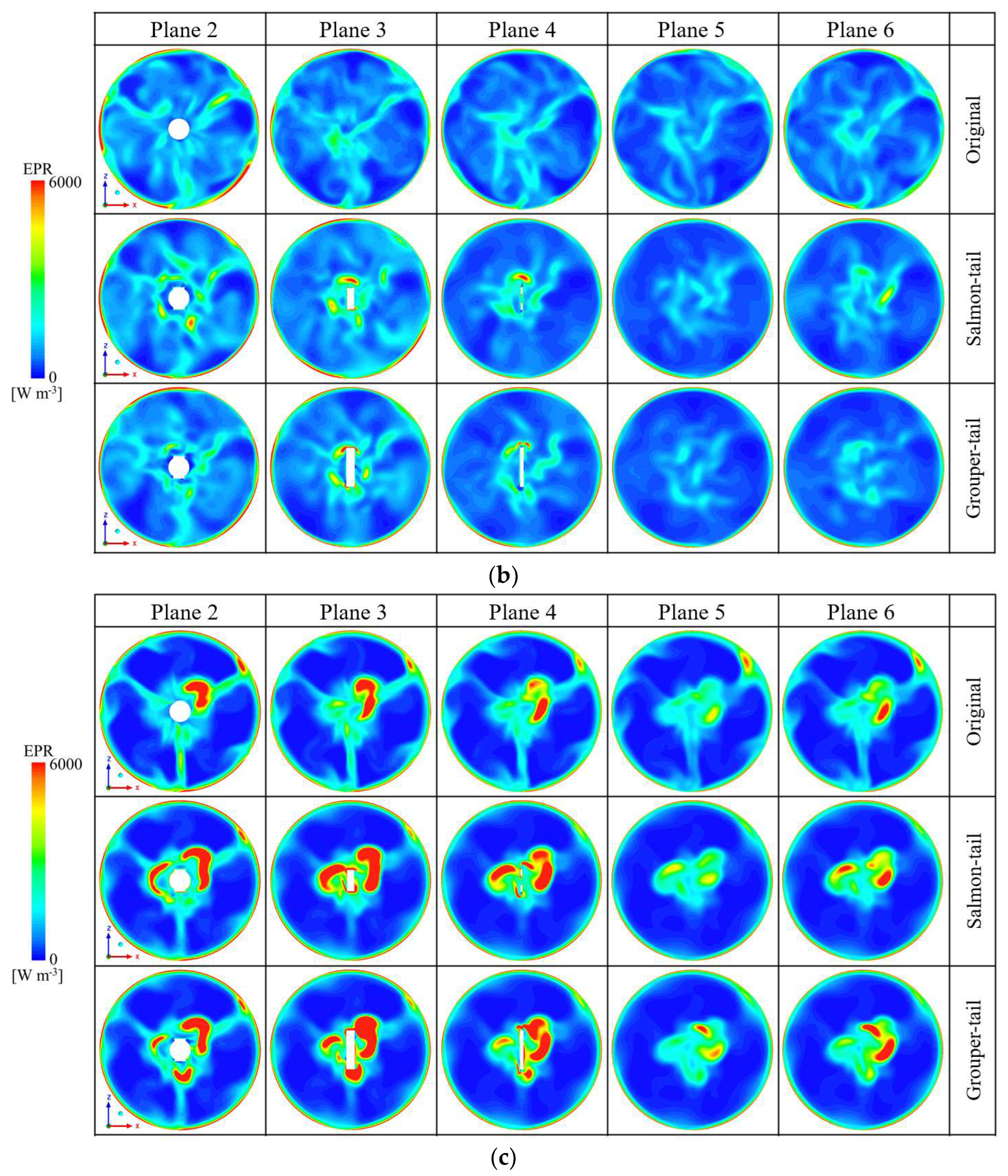
Figure 20 shows contours of the entropy production rate on normal sections of the outlet channel for the three configurations under different flow conditions. The figure mainly reflects local energy dissipation characteristics on different downstream sections near the rear of the bulb body and the fish tail. Overall, high-EPR regions under all conditions mainly appear near the rear of the bulb body, near the fish-tail structure, and close to the section walls. The annular high-value region near the wall is mainly associated with near-wall shear, whereas local high-value regions inside the section are mostly associated with wake disturbance, local vortices, and concentrated velocity gradients. From Plane 2 to Plane 6, high-EPR regions generally show a trend of being transported downstream from the region near the fish tail and gradually diffusing, but their intensity and decay characteristics differ markedly among flow rates.

At Q = 24 L/s, the high-EPR regions of the original configuration are mainly concentrated near the section boundaries and within the bulb body wake. The bionic fish-tail geometries introduce additional high-EPR regions near the tail surfaces in Planes 2–4, indicating enhanced local shear and energy dissipation. This effect is more pronounced for the salmon-tail configuration, whereas the grouper tail produces weaker and more localized high-EPR regions. Beyond Planes 5–6, these regions weaken markedly.

At Q = 30 L/s, the original configuration retains pronounced high-EPR regions on each section, indicating persistent downstream influence of the bulb body wake. The bionic geometries reduce the high-EPR regions in Planes 5–6, suggesting improved far-wake recovery and lower downstream dissipation. However, localized high-EPR regions appear near the fish-tail surfaces in Planes 3–4, especially for the salmon-tail configuration. The grouper tail produces weaker and more localized high-EPR regions, indicating smaller additional local losses.

At Q = 36 L/s, the high-EPR regions intensify markedly and persist from Planes 2 to 6, indicating stronger downstream transport of high-loss structures under the high-flow condition. In the original configuration, these regions are mainly concentrated within the bulb body wake and its downstream extension. The bionic geometries generate additional high-EPR regions near the fish-tail surfaces because of stronger interaction with the high-velocity incoming flow. This effect is most pronounced for the grouper-tail configuration, indicating greater local energy dissipation in the near-tail region.

Overall, the EPR distributions on the cross sections demonstrate that the effects of the bionic fish-tail geometries on local energy dissipation are strongly dependent on the operating condition. Under the low-flow condition, the bionic geometries mainly introduce additional losses in the near-tail region, particularly for the salmon-tail configuration. At the design flow rate, they reduce the downstream high-EPR regions, while the grouper tail induces weaker local disturbances. Under the high-flow condition, however, the near-tail high-EPR regions intensify markedly, with the grouper tail exhibiting greater local energy dissipation. Overall, the bionic fish-tail geometries can promote downstream wake recovery but may also introduce additional near-tail losses, with their net effects depending on both the operating condition and tail geometry.

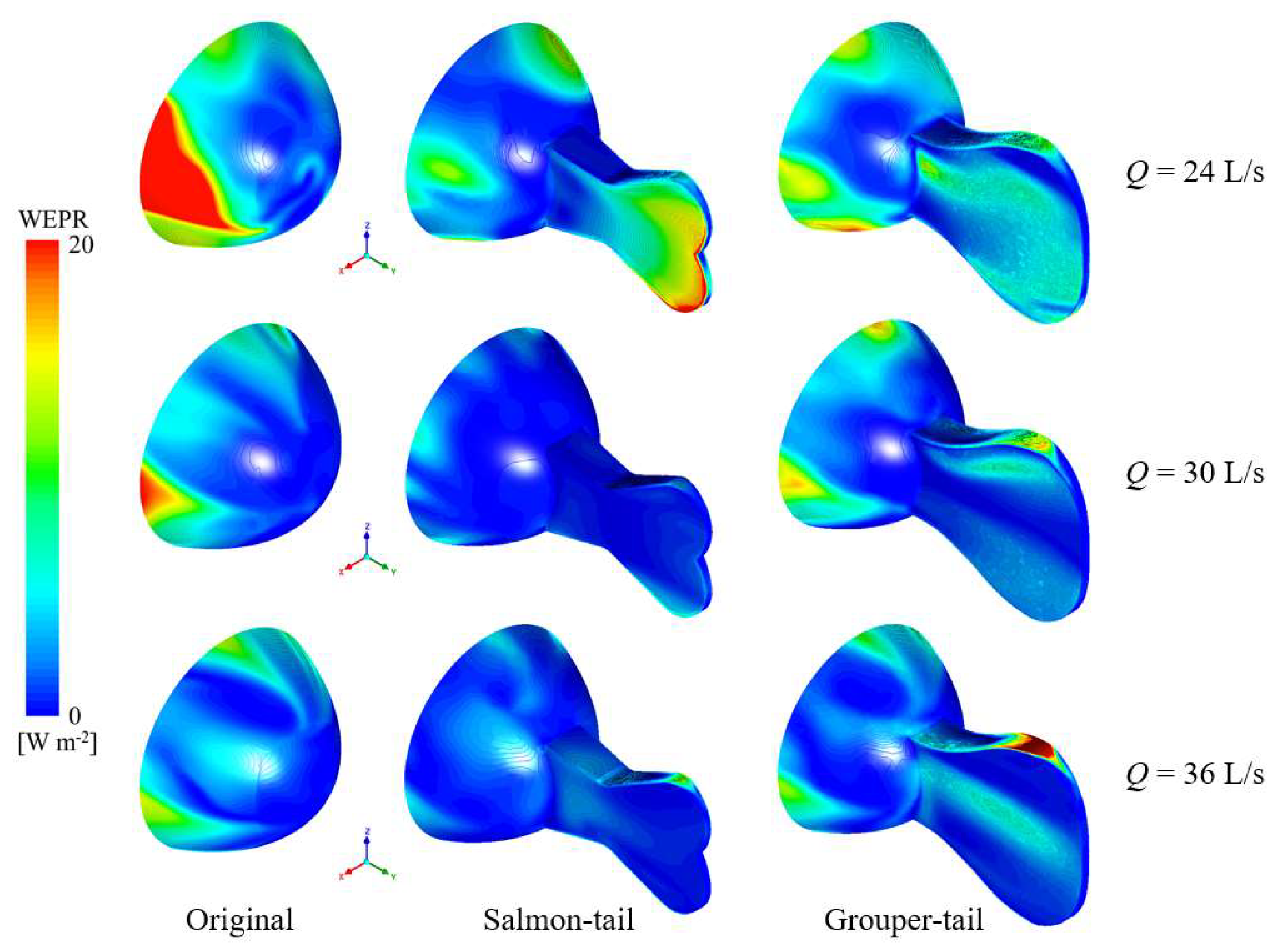
Figure 21 shows contours of wall entropy production rate (WEPR) on the fish-tail wall of the bulb body under different flow conditions. It should be noted that the maximum wall entropy production rate is approximately 20 W/m², whereas the maximum entropy production rate in the mainstream region discussed above reaches approximately 6000 W/m³. Although the two quantities have different dimensions and should not be directly compared numerically, the magnitude of local entropy production rates and the preceding loss decomposition results indicate that energy dissipation in the outlet channel is mainly concentrated inside the mainstream region, while wall loss is relatively small. Therefore, the WEPR contours are mainly used to identify the spatial distribution characteristics of shear loss on the fish-tail surface and local regions of the bulb body wall.

Under the low-flow condition of Q = 24 L/s, the high-WEPR region of the original configuration is mainly concentrated on the local lower side of the bulb body. After the fish-tail structure is introduced, new high-WEPR regions appear on the fish-tail surface and edges, indicating that the fish-tail geometry induces additional shear loss in the near-wall region. The salmon tail has obvious high-value regions at the tail end and edges, whereas the grouper tail has local high-value regions near the tail root and upper edge, indicating that both fish tails induce certain additional wall losses under low-flow conditions.

Under the design flow condition of Q = 30 L/s, the overall WEPR of all configurations decreases, and the range of high-value regions contracts markedly. The original configuration still has certain high values in local regions of the bulb body, whereas most fish-tail surfaces in the two fish-tail configurations remain at a low WEPR level, with only weak high-value regions near the tail root or local edges. This indicates that the fish-tail structure does not cause obvious additional wall loss at the design flow rate and that the near-wall flow state is relatively stable.

Under the high-flow condition of Q = 36 L/s, high-WEPR regions increase again. The high-value regions of the original configuration are mainly distributed on local surfaces of the bulb body, whereas those of the fish-tail configurations are more concentrated near the tail root and edge regions. This indicates that the interaction between the high-speed incoming flow and the fish-tail structure enhances local near-wall shear. The high-WEPR region near the upper edge and root of the grouper tail is more pronounced, indicating relatively greater induced local wall loss under high-flow conditions. The high-value region on the salmon-tail surface is relatively weaker, and wall shear dissipation is more dispersed.

Overall, the wall entropy production rate is much lower in magnitude than the entropy production rate in the mainstream region, indicating that wall loss is not the dominant source of energy dissipation in the outlet channel. The effect of the fish-tail structure on wall loss is mainly reflected in local shear enhancement, concentrated at the tail root, edges, and tail end. Its variation is strongly condition-dependent: additional local wall loss is more likely to form under low-flow and high-flow conditions, whereas the influence is weaker at the design flow rate.

5. Analysis of Pressure-Pulsation Characteristics

Pressure pulsation directly reflects the intensity and propagation characteristics of unsteady loads in the bulb tubular pump device and is a key indicator for evaluating operating stability and structural safety. The preceding sections have shown, from the perspectives of time-averaged flow structure and entropy production loss, that the bionic fish tail can change the bulb body wake, backflow region, and vortex-structure development. However, improvement in time-averaged performance does not necessarily mean that transient pressure load is reduced synchronously. Therefore, it is necessary to further establish a dynamic evaluation method based on pressure time series at multiple monitoring points and to reveal the regulation mechanism by which the bionic fish tail regulates pressure pulsation from four aspects: amplitude, frequency-band energy, spatial coherence, and phase organization.

5.1. Multidimensional Evaluation Method for Pressure Pulsation

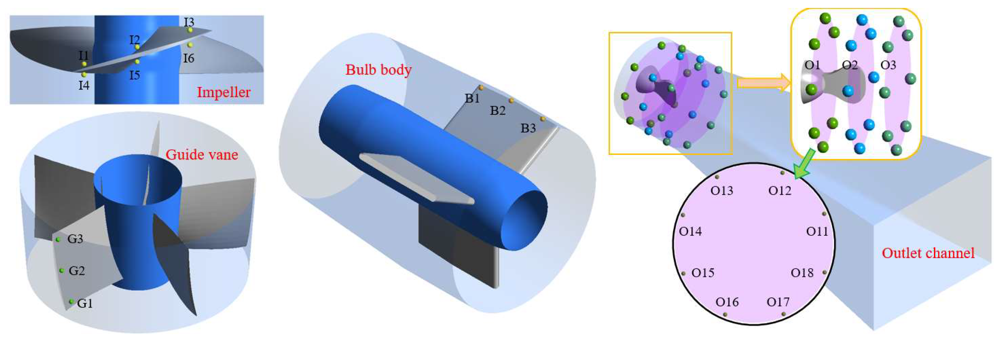
To clarify the spatial affiliation of pressure monitoring points, I/G/B/O prefixes were used to uniformly identify points in different regions, as shown in Figure 22. Here, I, G, B, and O denote monitoring points in the impeller domain, guide-vane domain, region near the bulb body and support, and outlet channel, respectively. The outlet conduit monitoring points are denoted as $Oij$, where $i$ is the row number and $j$ is the circumferential point number, forming three groups of outlet-section points: O11-O18, O21-O28, and O31-O38. This naming scheme is used in the figures and results discussion to maintain distinguishability among pressure responses in different spatial regions.

The last six impeller-rotation periods in the transient calculation were used as the statistical window for pressure pulsation to reduce the influence of the initial transition process on spectral and coherence results. Because the transient time step corresponds to 3 degrees of impeller rotation, each impeller period contains 120 sampling points, and the stable segment therefore contains 720 sampling points in total. To eliminate differences in static pressure levels among monitoring points, the transient pressure at each pressure monitoring point was first converted into a dimensionless pressure-pulsation coefficient:

$$C_{p\left(t\right)}^{\prime }={\displaystyle \frac{\left[p\left(t\right)-\overline{p}\right]}{0.5\rho u_2^2}},u_2={\displaystyle \frac{\pi Dn}{60}}$$

(31)

Here, $p\left(t\right)$ is the transient pressure, $\overline{p}$ is the time-averaged pressure within the statistical window, $\rho$ is the density of water, $u_2$ is the impeller circumferential velocity, $D$ is the impeller diameter, and $n$ is the impeller rotational speed. On this basis, the root-mean-square value $C_{p,rms}^{\prime }$ and peak-to-peak value $C_{p,pp}^{\prime }$ were used to characterize the pressure-pulsation amplitude:

$$C_{p,rms}^{\prime }={\left[N^{-1}\Sigma {\left(C_{p,i}^{\prime }\right)}^2\right]}^{0.5}$$

(32)

$$C_{p,pp}^{\prime }=\max \left(C_p^{\prime }\right)-\min \left(C_p^{\prime }\right)$$

(33)

Traditional pressure-pulsation analysis is usually centered on the dominant FFT frequency at a single monitoring point, which makes it difficult to reflect the spatial propagation characteristics of pressure waves among multiple monitoring points in the outlet channel. To improve the discriminative capability of the evaluation method, order energy decomposition was further constructed. Taking the impeller rotational frequency as the reference, the spectrum was divided into the low-order instability band (0.2$f_n$–1.5$f_n$), blade-passing band (2.5$f_n$–3.5$f_n$), guide-vane interference band (4.5$f_n$–5.5$f_n$), high-order harmonic band (5.5$f_n$–12$f_n$), and other frequency bands. The energy contribution of each band is defined as:

$$E_b=\Sigma f\in {\displaystyle \frac{b{A}^2\left(f\right)}{\Sigma 0.2f_n}}\le f\le 20f_n{A}^2\left(f\right)$$

(34)

Here, $A\left(f\right)$ is the spectral amplitude at frequency $f$. The low-order energy contribution reflects low-frequency instability caused by wake oscillation, unsteady development of the backflow region, and large-scale vortex shedding. The 3$f_n$ and 5$f_n$ energy contributions correspond to the main rotor-stator interference responses induced by the impeller blade number and guide-vane blade number, respectively. Meanwhile, normalized spectral entropy was introduced to evaluate the dispersion degree of pressure-pulsation energy among different orders:

$$H_s=-{\displaystyle \frac{\Sigma E_{m}ln\left(E_m\right)}{\mathit{ln}\left(M\right)}}$$

(35)

Here, $E_m$ is the normalized energy of the m-th order band, and $M$ is the number of orders included in the statistics. A larger $H_s$ indicates a more dispersed distribution of pressure-pulsation energy and more complex unsteady disturbance, whereas a smaller $H_s$ indicates that the pressure wave is more concentrated in regular order responses.

To further characterize spatial propagation of pressure pulsation among different monitoring points, a 3$f_n$ pressure-pulsation coherence network was established. The magnitude-squared coherence coefficient between any two monitoring points $i$ and $j$ is defined as:

$${\gamma }_{ij}^2\left(f\right)={\displaystyle \frac{{\left|G_{ij}\left(f\right)\right|}^2}{\left[G_{ii}\left(f\right)G_{jj}\left(f\right)\right]}}$$

(36)

Here, $G_{ij}\left(f\right)$ is the cross-power spectral density of the pressure-pulsation signals at the two monitoring points, and $G_{ii}\left(f\right)$ and $G_{jj}\left(f\right)$ are the auto-power spectral densities. When ${\gamma }_{ij}^2\left(f\right)$ approaches 1, the two monitoring points have a strong synchronous propagation relationship at that frequency; when ${\gamma }_{ij}^2\left(f\right)$ approaches 0, the coupling between them is weak. For the coherence calculation, the 720-sample statistical window was divided into six independent, non-overlapping one-revolution segments, with 120 samples in each segment. The cross-power and auto-power spectral densities in Equation (36) were obtained by averaging the corresponding Fourier coefficients over these six segments; therefore, $n_{seg}$ = 6 independent averaging segments were used for each magnitude-squared coherence estimate. Based on the coherence matrix, the high-coherence edge density is further defined as:

$$D_c=2{\left[n\left(n-1\right)\right]}^{-1}\Sigma I\left({\gamma }_{ij}^2\ge 0.8\right),i<j$$

(37)

A larger $D_c$ indicates that the 3$f_n$ pressure wave forms strong coupled propagation among more monitoring points and that the pressure disturbance has a more obvious whole-passage synchronization characteristic. In addition, to evaluate the degree of pressure-wave phase organization, the phases ${\phi }_i$ of the complex spectral coefficients at 3$f_n$ for all monitoring points were extracted, and the phase dispersion index was defined as:

$$PDI=1-\left|n^{-1}\Sigma \exp \left(j{\phi }_i\right)\right|$$

(38)

A larger PDI indicates a more dispersed 3$f_n$ phase distribution among different monitoring points, whereas a smaller PDI indicates stronger phase synchronization of the pressure wave. It should be noted that strong synchronization does not necessarily indicate better stability. When the pressure-pulsation amplitude is large and the coherence-network density is high, a lower PDI may correspond to a strong global pressure-wave propagation state.

By integrating the above indicators, this study proposes the dynamic pressure stability index (DPSI) to compare the unsteady pressure stability of different fish-tail configurations within the same dataset:

$$DPSI=0.35R^{*}+0.25E_{lo{w}^{*}}+0.20D_{c^{*}}+0.20PD{I}^{*}$$

(39)

Here, $R^{*}$, $E_{lo{w}^{*}}$,$D_{c^{*}}$, and $PD{I}^{*}$ are the normalized values over all operating conditions of $C_{p,rms}^{\prime }$, the low-order energy contribution, high-coherence edge density, and phase dispersion, respectively. A smaller DPSI indicates lower combined levels of pressure-pulsation amplitude, low-frequency instability, strong spatially coupled propagation, and phase dispersion. This index is not intended as a universal empirical formula, but as a relative stability evaluation metric for the three bulb body tail configurations under the same numerical settings and monitoring-point system in this study.

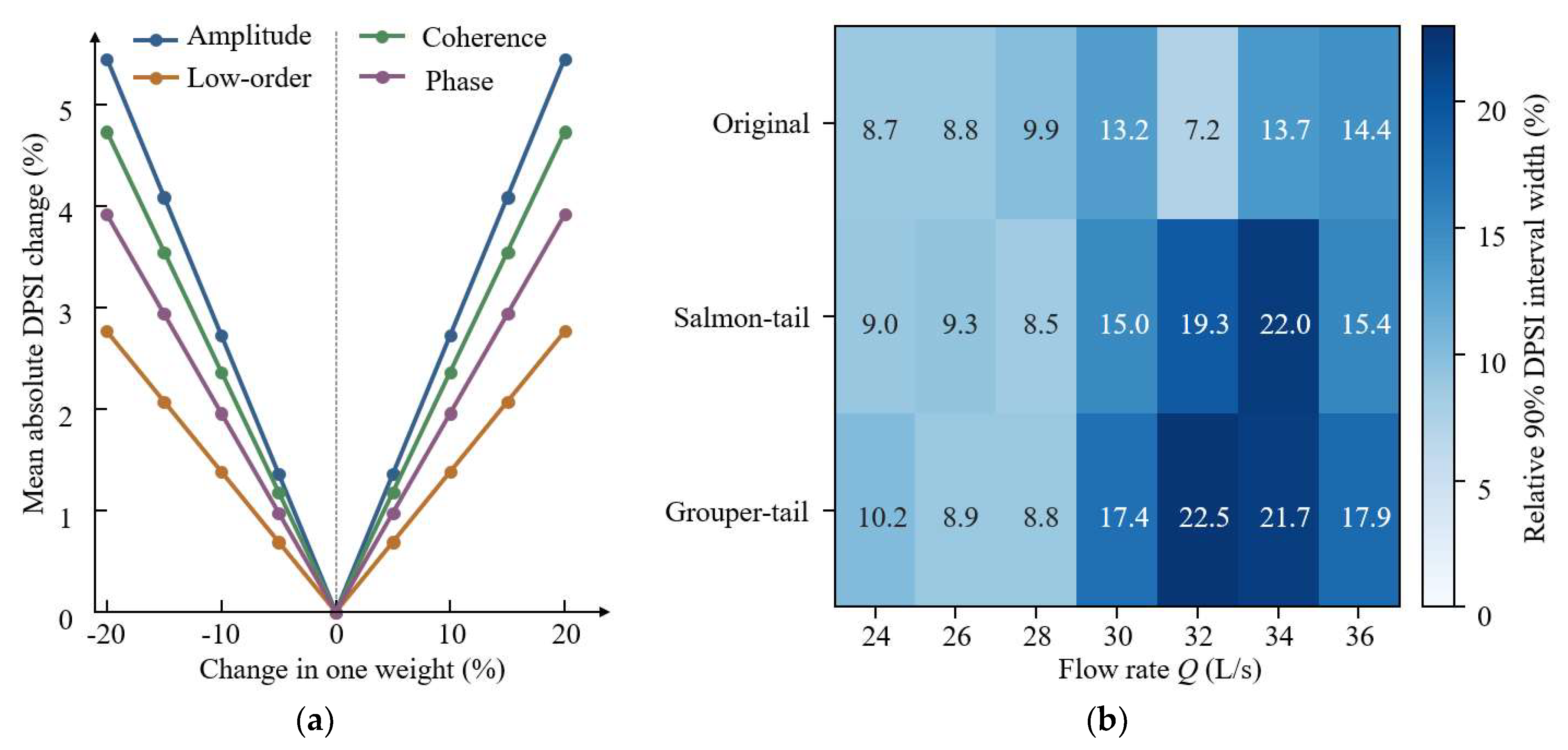
To examine the sensitivity of this composite index to the selected weights, a two-level coefficient-sensitivity analysis was further performed. In the one-at-a-time test, each baseline weight in Equation (39) was varied from −20% to +20% in 5% increments, while the other three weights were proportionally rescaled to keep the total weight equal to 1. The sensitivity was quantified by the mean absolute percentage change in DPSI relative to the baseline value over all 21 configuration–flow combinations. In the randomized test, 10,000 weight vectors were generated by independently perturbing the four baseline weights within ±20% and then renormalizing them. For each configuration and flow rate, the coefficient of variation and the 5th–95th percentile interval of the resulting DPSI distribution were calculated; the relative width of this interval was used to evaluate global weight sensitivity, and the configuration order was recorded as a secondary robustness check.

5.2. Time-Domain Amplitude and Spatial Distribution of Monitoring Points

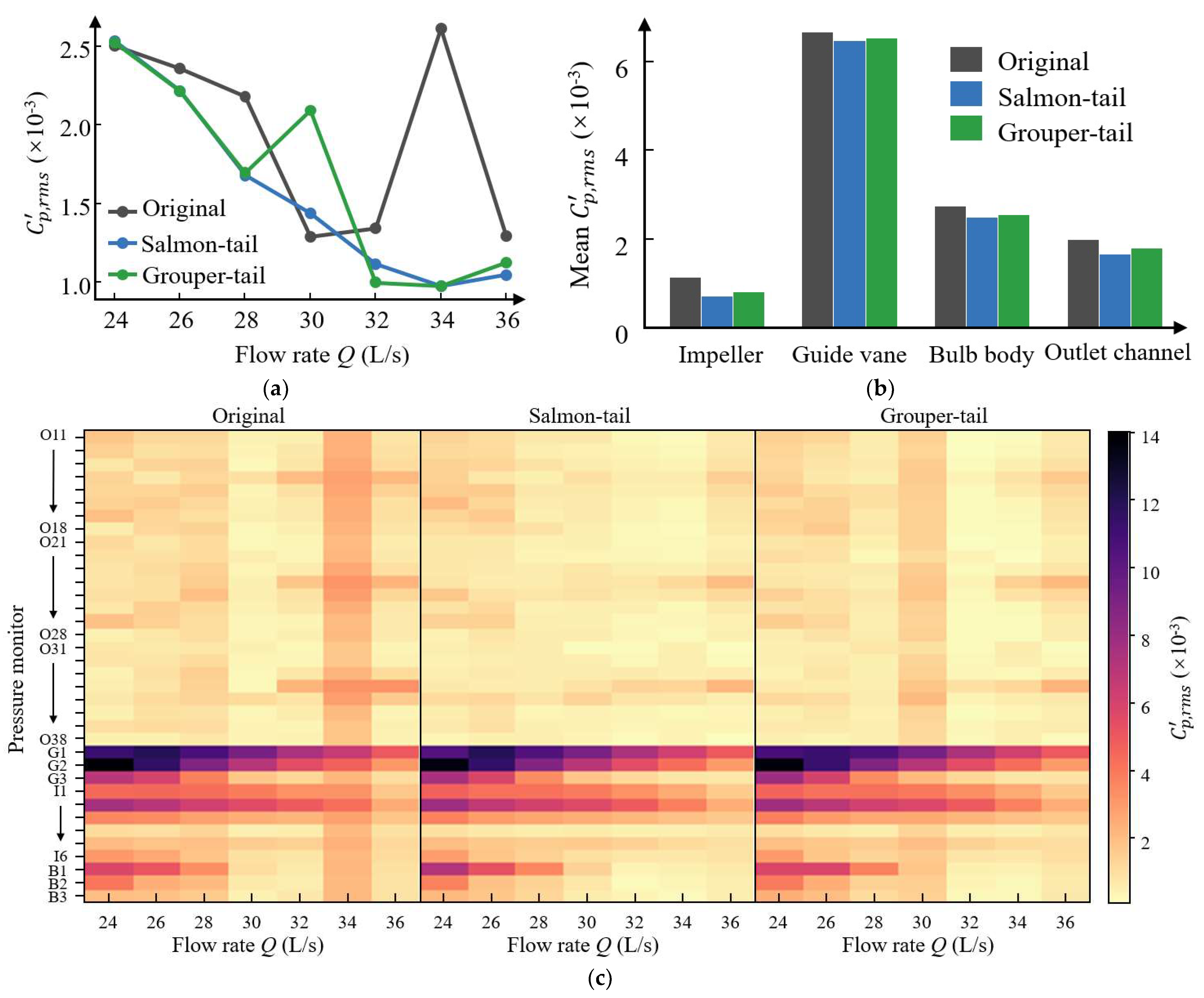
Figure 23 presents pressure-pulsation amplitude maps of the three tail configurations under different flow conditions. Overall, pressure-pulsation amplitude varies nonmonotonically with flow rate, indicating that pressure stability in the outlet channel is controlled not only by flow rate magnitude but also by the bulb body wake, backflow-region scale, and propagation of local vortex structures. From the averaged results of monitoring-point groups, the G group (guide-vane domain) has the strongest pressure pulsation, with an average value clearly higher than those of the I group (impeller domain), B group (bulb body), and O group (outlet channel), indicating that the guide-vane domain and its downstream wake-coupling region are the areas where the pressure-pulsation response is strongest.

At Q = 34 L/s, the overall $C_{p,rms}^{\prime }$ of the original configuration reaches 2.61 × 10⁻³, whereas those of the salmon-tail and grouper-tail configurations are reduced by 62.68% and 62.53%, respectively, relative to the original configuration. This indicates that the bionic fish-tail geometries can significantly suppress pressure-pulsation amplitudes under this relatively high-flow condition, particularly at monitoring points exhibiting strong pulsations. At Q = 32 L/s, the salmon-tail and grouper-tail configurations reduce the overall $C_{p,rms}^{\prime }$ by 17.02% and 25.62%, respectively, while at Q = 36 L/s, the corresponding reductions are 19.24% and 13.05%.

It Is worth noting that Q = 30 L/s near the design flow rate does not show a simple pressure stabilization gain. The overall $C_{p,rms}^{\prime }$ values of the salmon-tail and grouper-tail configurations increase by 11.29% and 62.04%, respectively, compared with the original configuration. This result indicates that the flow-straightening and loss-reduction effects of the fish-tail structure on time-averaged flow is not always synchronized with the suppression of transient pressure loads. In other words, while improving wake diffusion and reducing entropy production loss, the bionic fish tail may enhance local blade-passing pressure response under certain conditions. Therefore, pressure-pulsation evaluation cannot rely only on time-averaged efficiency or entropy production results; order energy and spatial propagation indicators must be introduced for comprehensive assessment.

5.3. Order-Energy Decomposition and Spectral Complexity

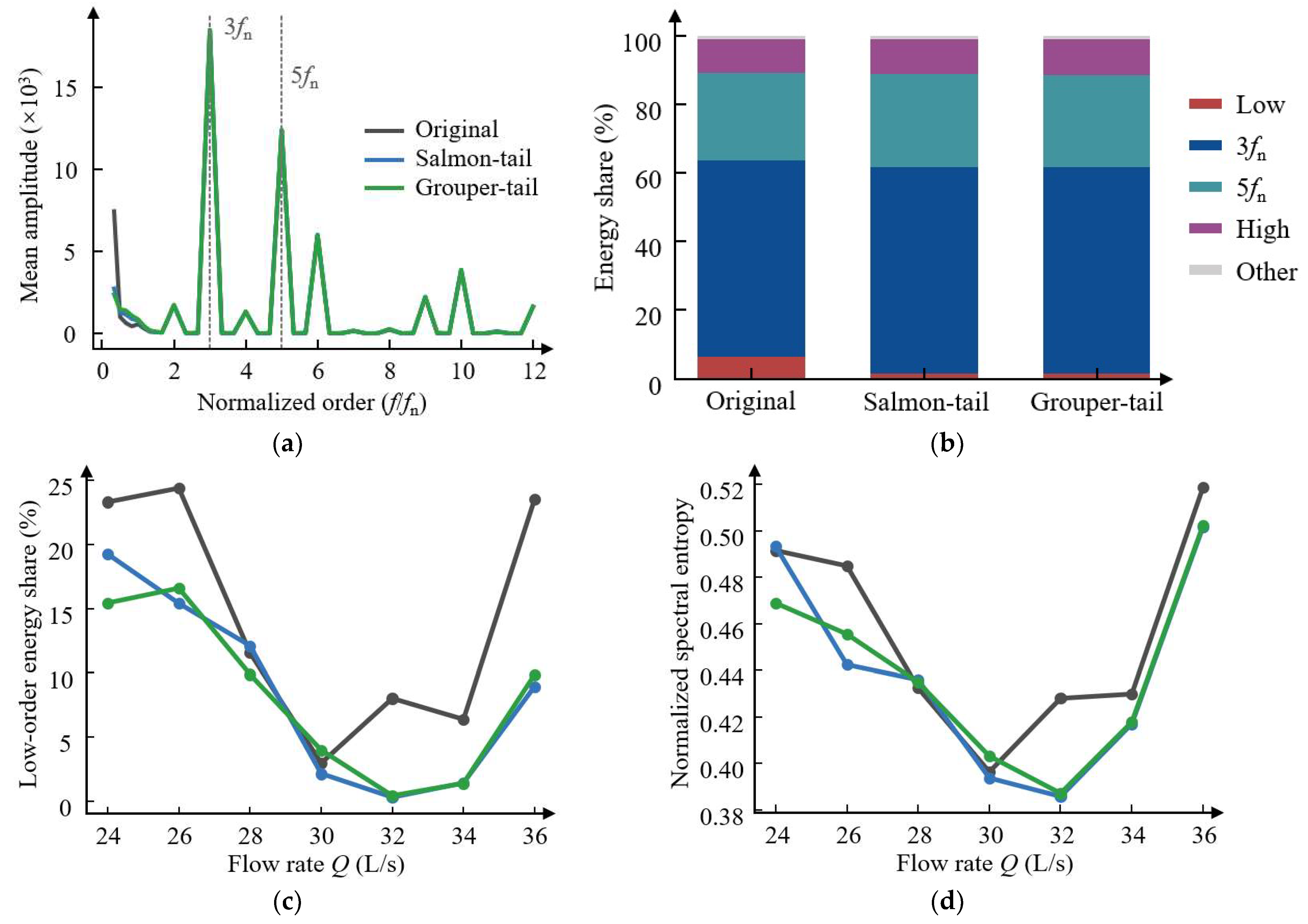
Figure 24 further presents the order energy decomposition results for pressure pulsation. Under most operating conditions, all three configurations show obvious 3$f_n$ and 5$f_n$ responses, where 3$f_n$ corresponds to the number of impeller blades and 5fn corresponds to the number of guide-vane blades. This indicates that the dominant excitation of pressure pulsation in the bulb tubular pump still originates from impeller–guide vane rotor–stator interaction. The bionic fish tail does not change the dominant pressure-pulsation orders, but mainly changes the energy contributions of different orders and the intensity of low-order unstable components. Taking Q = 34 L/s as an example, the low-order energy contribution of the original configuration is 6.39%, whereas those of the salmon-tail and grouper-tail configurations decrease to 1.41% and 1.39%, respectively. This indicates that the bionic fish tail effectively weakens low-order disturbances related to large-scale wake oscillation and unsteady development of the backflow region under this condition. Meanwhile, the spectral entropy decreases from 0.430 for the original configuration to 0.417 for the salmon tail and 0.418 for the grouper tail, indicating that the pressure-pulsation energy distribution becomes more concentrated and that randomness and complexity are reduced.

Over the full flow rate range, the original configuration has a relatively high low-order energy contribution under low-flow conditions, indicating that backflow and wake oscillation contribute more strongly to pressure pulsation at a low flow rate. Near the design flow rate, low-order energy decreases markedly, and pressure pulsation is mainly concentrated in regular blade-passing and guide-vane interference orders. When the flow rate further increases to Q = 36 L/s, low-order energy and spectral entropy increase again, indicating that after mainstream inertia is enhanced at a high flow rate, wake-vortex shedding and downstream transport re-excite broadband unsteady responses. This pattern is consistent with the preceding vortex structure and entropy production analyses, which showed enhanced local disturbance under high-flow conditions.

5.4. Pressure Wave Spatial Coherence and Phase Propagation

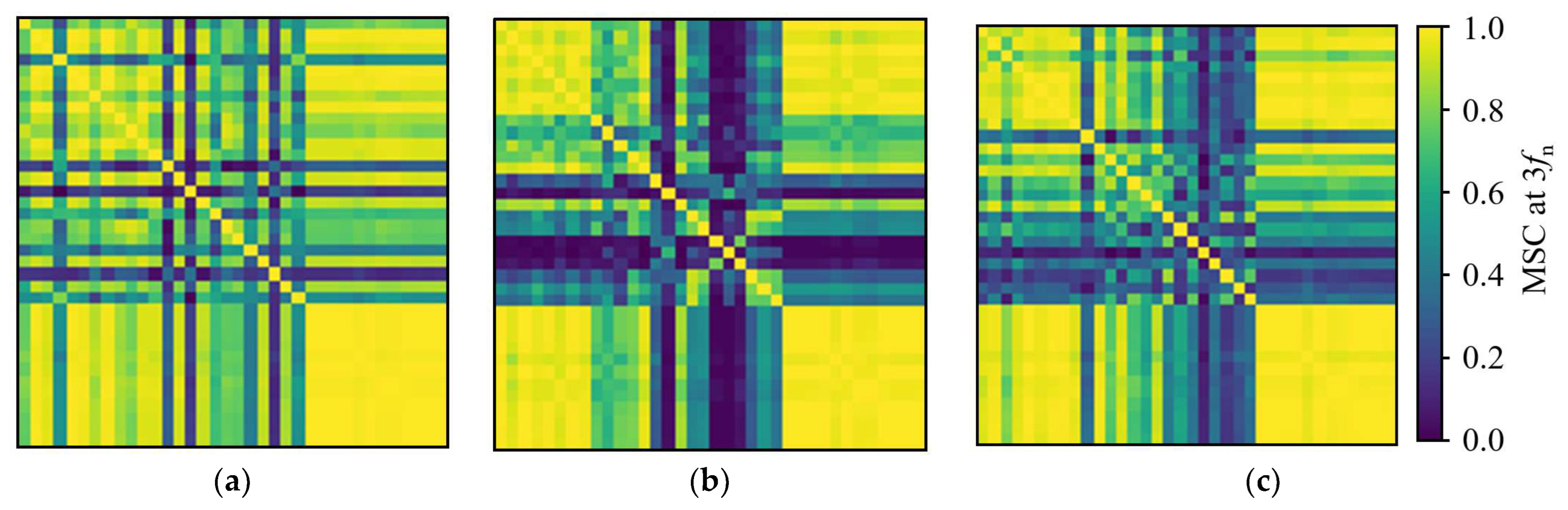
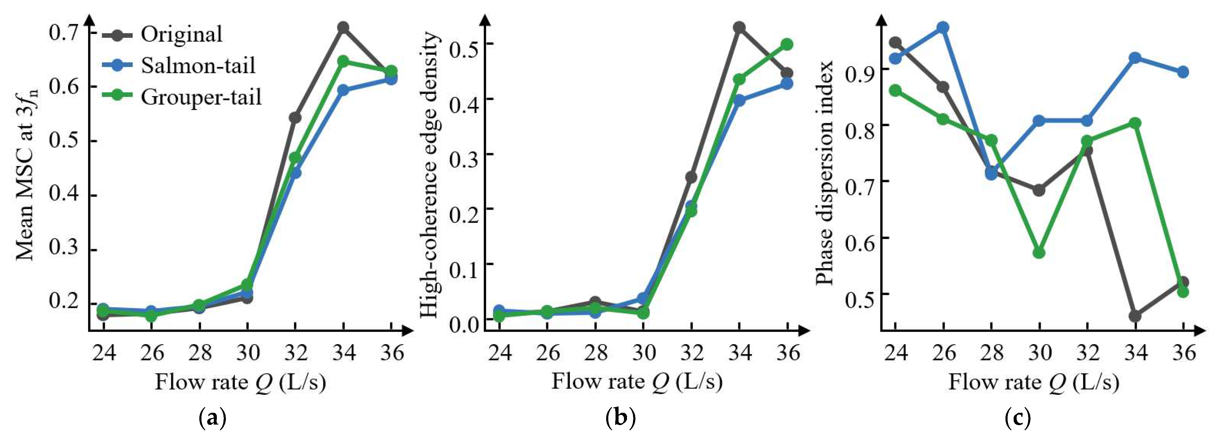
To further reveal the spatial propagation characteristics of pressure pulsation among multiple monitoring points, a pressure-pulsation coherence network was constructed for the dominant blade-passing frequency. Figure 25 shows the 3$f_n$ magnitude-squared coherence matrices of the three configurations at Q = 34 L/s. In the original configuration, broad high-coherence regions exist among multiple monitoring-point zones, indicating that strong blade-passing pressure waves can form widespread synchronous propagation in the outlet channel. After the fish-tail structure is introduced, the high-coherence regions are weakened and become more localized, indicating that the bionic fish tail weakens the overall coupled propagation of pressure waves from the near-wake region to downstream monitoring points. To further quantify the evolution of pressure-wave spatial coupling over the entire flow range, Figure 26 presents the mean magnitude-squared coherence (MSC) at 3$f_n$, high-coherence edge density $D_c$, and phase dispersion index (PDI) for the three configurations.

As shown in Figure 26a,b, both the mean MSC and $D_c$ increase markedly when Q exceeds 30–32 L/s, indicating enhanced spatial coupling of blade-passing pressure waves at high flow rates. At Q = 34 L/s, $D_c$ reaches 0.529 for the original configuration, whereas it decreases to 0.397 and 0.435 for the salmon-tail and grouper-tail configurations, respectively. Combined with the coherence matrices in Figure 25, these results demonstrate that the bionic geometries not only reduce the pressure-pulsation amplitude but also restrict the spatial coupling range of the dominant blade-passing pressure wave.

Figure 26c further shows that the phase-propagation characteristics vary considerably with flow rate and bulb body geometry. At Q = 34 L/s, the original configuration exhibits a lower PDI but simultaneously has a higher pressure-pulsation amplitude and a denser high-coherence network. This combination indicates that the low PDI does not represent a weakly disturbed state; rather, it reflects a strongly synchronized global blade-passing pressure wave. In contrast, the bionic configurations reduce both the pulsation amplitude and coherence-network density while increasing phase dispersion, indicating that the originally strong global pressure response is reorganized into weaker and more localized fluctuations. Therefore, pressure-pulsation stability should be evaluated by jointly considering amplitude, spatial coherence, and phase organization rather than phase synchronization alone.

5.5. Comprehensive Evaluation of Dynamic Pressure Stability

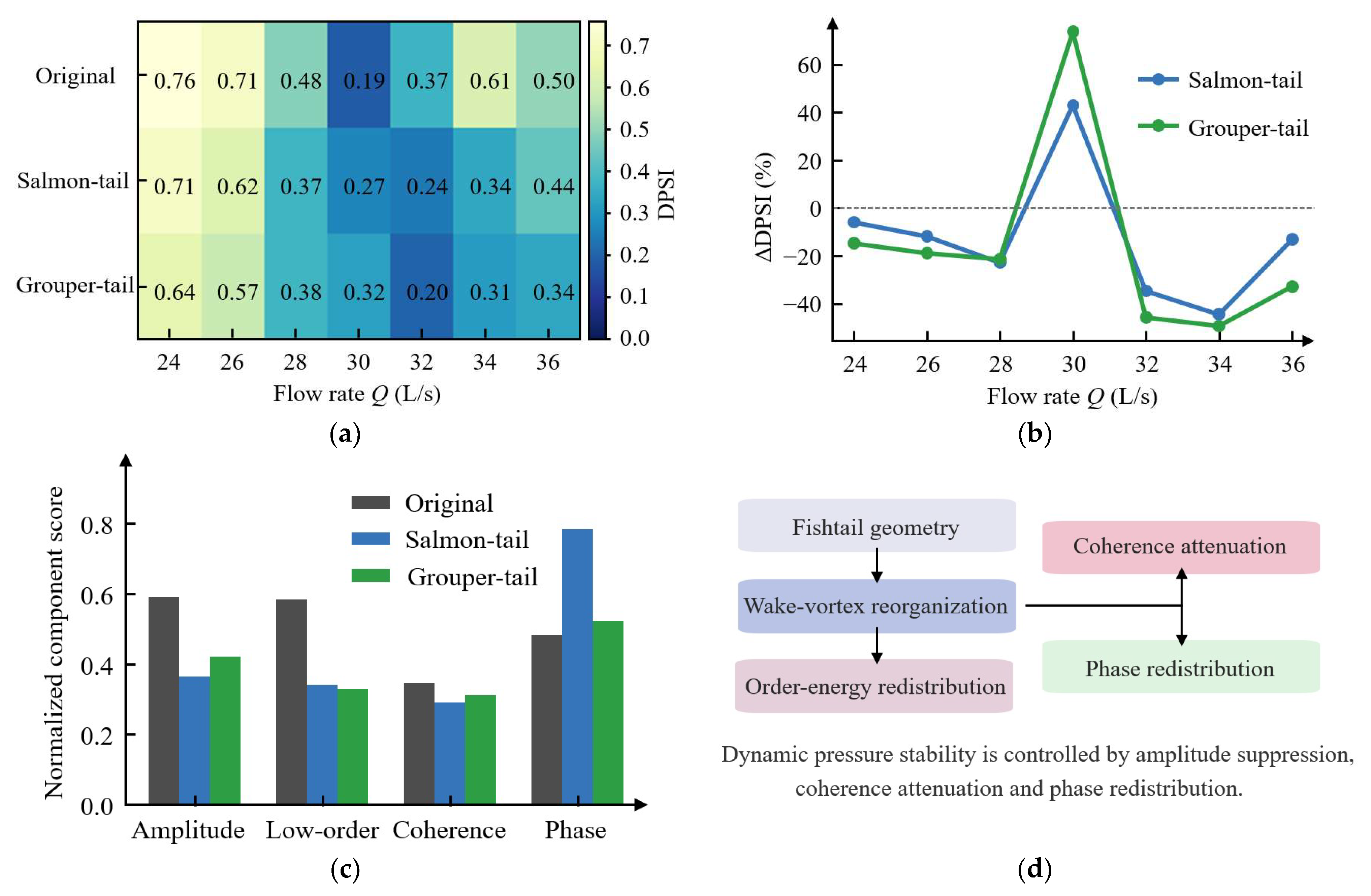
Based on amplitude intensity, low-order energy contribution, high-coherence edge density, and phase dispersion, the DPSI was further calculated to comprehensively evaluate the dynamic pressure stability of different fish-tail configurations. As shown in Figure 27, DPSI varies markedly with flow rate and fish-tail morphology, indicating that the regulation of pressure pulsation by the bionic fish tail is strongly condition-dependent. At Q = 34 L/s, the DPSI of the original configuration is 0.613, whereas those of the salmon-tail and grouper-tail configurations decrease to 0.340 and 0.310, respectively, corresponding to relative reductions of 44.49% and 49.39%. This indicates that under relatively high-flow conditions, the fish-tail structure can improve the dynamic pressure stability of the device by simultaneously reducing pressure-pulsation amplitude, low-order energy, and the intensity of spatially coherent propagation.

However, at Q = 30 L/s, the DPSI of the original configuration is 0.186, lower than 0.266 for the salmon tail and 0.323 for the grouper tail. This indicates that although the fish-tail structure may improve time-averaged flow or local energy loss near the design flow rate, the interaction between its geometric edges and the incoming flow may also enhance local pressure-wave response. Therefore, the DPSI proposed in this study can reveal the “efficiency improvement-pressure stabilization” trade-off that is difficult to identify using traditional time-averaged performance indicators.

Taken together, Figure 23, Figure 24, Figure 25, Figure 26 and Figure 27 show that the influence of the bionic fish tail on pressure pulsation is not a simple reduction across all operating conditions, but is expressed as a coupled effect of amplitude suppression, frequency-band energy redistribution, spatial coherence attenuation, and phase reconstruction. The grouper tail shows lower DPSI values in the range of Q = 32–36 L/s, indicating more stable dynamic pressure stabilization capability at medium to relatively high flow rates. The salmon tail also significantly reduces pressure-pulsation amplitude and low-order energy at Q = 34 L/s, but its phase dispersion is higher, indicating a stronger pressure-wave reconstruction process. Combined with the preceding results on the backflow region, vortex structure, and entropy production, the bionic fish tail can be considered to weaken low-order unsteady disturbance and spatially coupled propagation of pressure waves by changing the vortex-structure transport process in the bulb body wake. However, when the interaction between the fish-tail geometry and the mainstream is excessively strong, additional local pressure waves may also be induced. Therefore, optimization of the bionic fish tail should not pursue only improvement in time-averaged efficiency but should also constrain dynamic pressure stability.

To test whether the DPSI-based comparison depends on the selected coefficient scheme, the weight-sensitivity results are summarized in Figure 28 and

Table 4. DPSI sensitivity under ±20% randomized weight perturbations.

Q (L/s)	Mean 90% Width (%)	Max 90% Width (%)	Max CV (%)
24	9.29	10.16	3.05
26	9.00	9.29	2.85
28	9.06	9.92	2.99
30	15.20	17.37	5.34
32	16.33	22.55	6.89
34	19.16	22.00	6.68
36	15.91	17.88	5.45

. The one-at-a-time perturbation produced a smooth DPSI response. At the ±20% endpoints, changes in the amplitude, low-order energy, coherence, and phase weights caused mean absolute DPSI changes of 5.45%, 2.76%, 4.73%, and 3.91%, respectively, across the 21 configuration–flow combinations. In the randomized-weight analysis, the relative width of the 5th–95th percentile DPSI interval ranged from 7.20% to 22.55%, and the maximum coefficient of variation was 6.89%. The original configuration order was unchanged in all one-at-a-time perturbations. In the 10,000 randomized tests, the baseline best configuration was retained in 100% of samples at six flow rates and 96.39% at Q = 28 L/s, where the salmon-tail and grouper-tail DPSI values were nearly equal. These results indicate that the DPSI ranking is robust within the tested coefficient range and is not mainly determined by the chosen weights.

6. Conclusions

This study compared the effects of the original bulb body, salmon-tail bulb body, and grouper-tail bulb body on the tail flow, entropy production loss, and pressure pulsation of a bulb tubular pump. The main conclusions are as follows:

(1)

The bionic fish tail improves time-averaged energy performance and wake structure in the medium-to-high relative flow rate range while largely maintaining the head curve. The two fish-tail configurations generally show positive gains in the range of 0.93–1.13 $Q_{des}$, with the grouper tail providing more stable head and efficiency gains. At 0.80 $Q_{des}$, the salmon tail and grouper tail reduce the vortex-structure volume fraction from 2.69% to 1.65% and 1.71%, respectively, indicating that the fish-tail structure can weaken vortex development induced by flow separation behind the bulb body.

(2)

The entropy production results show that the bionic fish tail does not change the overall pattern in which losses are dominated by the impeller region, but it can regulate local energy loss in the outlet channel. The entropy production power contribution of the impeller region is approximately 52–67% for all configurations, whereas the entropy production contribution of the outlet channel increases from approximately 7–8% to 17–19% as the relative flow rate increases. The two fish-tail configurations reduce the total entropy production power of the outlet channel under most operating conditions, and the grouper tail shows more stable loss-reduction capability. However, the tail root, edges, and tail end may still induce local additional shear loss.

(3)

The pressure-pulsation results show that the improvement in dynamic stability provided by the bionic fish tail is strongly condition-dependent. At 1.13 $Q_{des}$, the salmon tail and grouper tail reduce the overall pressure-pulsation amplitude by 62.68% and 62.53%, respectively, reduce the low-order energy contributions to 1.41% and 1.39%, respectively, and decrease the dynamic pressure stability index by 44.49% and 49.39%, respectively. In contrast, at $Q_{des}$, the DPSI increases from 0.186 for the original configuration to 0.266 and 0.323 for the salmon-tail and grouper-tail configurations, respectively, indicating deteriorated dynamic pressure stability. The results indicate that the fish-tail structure can weaken low-order unsteady disturbance and the spatially coupled propagation of strong blade-passing pressure waves at relatively high flow rates, but does not universally improve pressure stability across all operating conditions.

Overall, the mechanism of the bionic fish-tail bulb body can be summarized as “wake reconstruction-entropy production migration-pressure-wave reorganization”. The fish-tail structure can reduce energy dissipation and pressure-wave propagation intensity in the outlet channel at medium-to-high relative flow rates, but when the interaction between the fish-tail geometry and the mainstream is too strong, additional local loss and pressure-wave response may also occur. Therefore, bionic fish-tail optimization should not focus only on improving time-averaged efficiency, but should also constrain dynamic pressure stability.

References

1. Qin, J.; Duan, W.; Zou, S.; Chen, Y.; Huang, W.; Rosa, L. Global energy use and carbon emissions from irrigated agriculture. Nat. Commun. 2024, 15, 3084. [Google Scholar] [CrossRef] [Scilit] [PubMed]
2. Siyal, A.W.; Gerbens-Leenes, P.W. The water-energy nexus in irrigated agriculture in South Asia: Critical hotspots of irrigation water use, related energy application, and greenhouse gas emissions for wheat, rice, sugarcane, and cotton in Pakistan. Front. Water 2022, 4, 941722. [Google Scholar] [CrossRef] [Scilit]
3. Sun, L.; Pan, Q.; Zhang, D.; Zhao, R.; van Esch, B.P.M. Numerical study of the energy loss in the bulb tubular pump system focusing on the off-design conditions based on combined energy analysis methods. Energy 2022, 258, 124794. [Google Scholar] [CrossRef] [Scilit]
4. Tian, X.; Cheng, L.; Jiao, W.; Wang, Y.; Luo, C. Analysis of internal flow characteristics and entropy generation of low head bulb tubular pump. Front. Energy Res. 2023, 11, 1183086. [Google Scholar] [CrossRef] [Scilit]
5. Shi, L.; Yuan, Y.; Jiao, H.; Tang, F.; Cheng, L.; Yang, F. Numerical investigation and experiment on pressure pulsation characteristics in a full tubular pump. Renew. Energy 2021, 163, 987–1000. [Google Scholar] [CrossRef] [Scilit]
6. Wang, J.; Chen, Z.; Li, L.; Wang, C.; Teng, K.; He, Q. Pressure Pulsation Characteristics on the Bulb Body of a Submersible Tubular Pump. Water 2024, 16, 789. [Google Scholar] [CrossRef] [Scilit]
7. Ji, D.; Lu, W.; Xu, L.; Lu, L. Comparison of the Hydraulic Performance and Pressure Pulsation Characteristics of Shaft Tubular Pump Device under Multiple Working Conditions. J. Mar. Sci. Eng. 2022, 10, 750. [Google Scholar] [CrossRef] [Scilit]
8. Sun, Z.; Yu, J.; Tang, F. The Influence of Bulb Position on Hydraulic Performance of Submersible Tubular Pump Device. J. Mar. Sci. Eng. 2021, 9, 831. [Google Scholar] [CrossRef] [Scilit]
9. Ji, D.; Lu, W.; Lu, L.; Xu, L.; Liu, J.; Shi, W. Study on the Comparison of the Hydraulic Performance and Pressure Pulsation Characteristics of a Shaft Front-Positioned and a Shaft Rear-Positioned Tubular Pump Devices. J. Mar. Sci. Eng. 2021, 10, 8. [Google Scholar] [CrossRef] [Scilit]
10. Wang, B.; Wang, H.; Wang, F.; Wang, C. Pressure polarization oscillation in large-scale bulb tubular pump. Phys. Fluids 2023, 35, 055104. [Google Scholar] [CrossRef] [Scilit]
11. Sun, S.; Jin, X.; Lin, Z.; Shao, C.; Wang, H.; Yang, F. Analysis of flow characteristics and pressure pulsation in impeller region of shaft tubular pump device with different tip clearances. AIP Adv. 2024, 14, 125109. [Google Scholar] [CrossRef] [Scilit]
12. Lv, Y.; Ding, P.; Liu, J.; Ge, H.; Yang, F.; Tang, F. Numerical analysis of the internal flow and pressure pulsation characteristics of a submersible tubular electric pump device. Front. Energy Res. 2023, 10, 1104248. [Google Scholar] [CrossRef] [Scilit]
13. Bai, Y.; Wu, D. Test and Numerical Simulation of Pressure Pulsation under the Forward and Reverse Working Conditions of a Horizontal Axial Flow Pump. Appl. Sci. 2022, 12, 12956. [Google Scholar] [CrossRef] [Scilit]
14. Jiang, D.; Yang, F.; Cai, Y.; Xu, G.; Tang, F.; Jin, Y. Cross influence of rotational speed and flow rate on pressure pulsation and hydraulic noise of an axial-flow pump. Phys. Fluids 2023, 35, 095144. [Google Scholar] [CrossRef] [Scilit]
15. Yang, F.; Chang, P.; Hu, W.; Mao, B.; Liu, C.; Li, Z. Numerical Study on Pressure Pulsation in a Slanted Axial-Flow Pump Device under Partial Loads. Processes 2021, 9, 1404. [Google Scholar] [CrossRef] [Scilit]
16. Song, X.; Liu, C. Experimental investigation of floor-attached vortex effects on the pressure pulsation at the bottom of the axial flow pump sump. Renew. Energy 2020, 145, 2327–2336. [Google Scholar] [CrossRef] [Scilit]
17. Zhang, N.; Gao, B.; Ni, D.; Liu, X. Coherence analysis to detect unsteady rotating stall phenomenon based on pressure pulsation signals of a centrifugal pump. Mech. Syst. Signal Process. 2021, 148, 107161. [Google Scholar] [CrossRef] [Scilit]
18. Wu, C.; Zhang, W.; Wu, P.; Yi, J.; Ye, H.; Huang, B. Effects of Blade Pressure Side Modification on Unsteady Pressure Pulsation and Flow Structures in a Centrifugal Pump. J. Fluids Eng. 2021, 143, 111208. [Google Scholar] [CrossRef] [Scilit]
19. Shi, F.; Tsukamoto, H. Numerical Study of Pressure Fluctuations Caused by Impeller-Diffuser Interaction in a Diffuser Pump Stage. J. Fluids Eng. 2001, 123, 466–474. [Google Scholar] [CrossRef] [Scilit]
20. Kock, F.; Herwig, H. Local entropy production in turbulent shear flows: A high-Reynolds number model with wall functions. Int. J. Heat Mass Transf. 2004, 47, 2205–2215. [Google Scholar] [CrossRef] [Scilit]
21. Kock, F.; Herwig, H. Entropy production calculation for turbulent shear flows and their implementation in CFD codes. Int. J. Heat Fluid Flow 2005, 26, 672–680. [Google Scholar] [CrossRef] [Scilit]
22. Herwig, H.; Kock, F. Direct and indirect methods of calculating entropy generation rates in turbulent convective heat transfer problems. Heat Mass Transf. 2006, 43, 207–215. [Google Scholar] [CrossRef] [Scilit]
23. Fan, B.; Liang, Z.; Fan, R.; Chen, S. Numerical Study on Entropy Generation of the Multi-Stage Centrifugal Pump. Entropy 2022, 24, 923. [Google Scholar] [CrossRef] [Scilit] [PubMed]
24. Cui, B.; Zhang, C. Investigation on Energy Loss in Centrifugal Pump Based on Entropy Generation and High-Order Spectrum Analysis. J. Fluids Eng. 2020, 142, 091205. [Google Scholar] [CrossRef] [Scilit]
25. Tang, X.; Jiang, W.; Li, Q.; Hou, G.; Zhang, N.; Wang, Y. Analysis of hydraulic loss of the centrifugal pump as turbine based on internal flow feature and entropy generation theory. Sustain. Energy Technol. Assess. 2022, 52, 102070. [Google Scholar] [CrossRef] [Scilit]
26. Lin, P.; Wang, C.; Song, P.; Li, X. Analysis of the Energy Loss and Performance Characteristics in a Centrifugal Pump Based on Sinusoidal Tubercle Volute Tongue. Entropy 2023, 25, 545. [Google Scholar] [CrossRef] [Scilit] [PubMed]
27. Choi, H.; Jeon, W.-P.; Kim, J. Control of Flow Over a Bluff Body. Annu. Rev. Fluid Mech. 2008, 40, 113–139. [Google Scholar] [CrossRef] [Scilit]
28. Beaudoin, J.-F.; Cadot, O.; Aider, J.-L.; Wesfreid, J.-E. Drag reduction of a bluff body using adaptive control methods. Phys. Fluids 2006, 18, 085107. [Google Scholar] [CrossRef] [Scilit]
29. Beaudoin, J.F.; Cadot, O.; Aider, J.L.; Wesfreid, J.E. Bluff-body drag reduction by extremum-seeking control. J. Fluids Struct. 2006, 22, 973–978. [Google Scholar] [CrossRef] [Scilit]
30. Triantafyllou, M.S.; Triantafyllou, G.S.; Yue, D.K.P. Hydrodynamics of Fishlike Swimming. Annu. Rev. Fluid Mech. 2000, 32, 33–53. [Google Scholar] [CrossRef] [Scilit]
31. Lauder, G.V.; Drucker, E.G. Morphology and Experimental Hydrodynamics of Fish Fin Control Surfaces. IEEE J. Ocean. Eng. 2004, 29, 556–571. [Google Scholar] [CrossRef] [Scilit]
32. Drucker, E.G.; Lauder, G.V. Locomotor function of the dorsal fin in teleost fishes: Experimental analysis of wake forces in sunfish. J. Exp. Biol. 2001, 204, 2943–2958. [Google Scholar] [CrossRef] [Scilit] [PubMed]
33. Nauen, J.C.; Lauder, G.V. Hydrodynamics of caudal fin locomotion by chub mackerel, Scomber japonicus (Scombridae). J. Exp. Biol. 2002, 205, 1709–1724. [Google Scholar] [CrossRef] [Scilit] [PubMed]
34. Drucker, E.G.; Lauder, G.V. Locomotor forces on a swimming fish: Three-dimensional vortex wake dynamics quantified using digital particle image velocimetry. J. Exp. Biol. 1999, 202, 2393–2412. [Google Scholar] [CrossRef] [Scilit] [PubMed]
35. Ren, Z.; Yang, X.; Wang, T.; Wen, L. Hydrodynamics of a robotic fish tail: Effects of the caudal peduncle, fin ray motions and the flow speed. Bioinspir. Biomim. 2016, 11, 016008. [Google Scholar] [CrossRef] [Scilit] [PubMed]
36. Han, P.; Lauder, G.V.; Dong, H. Hydrodynamics of median-fin interactions in fish-like locomotion: Effects of fin shape and movement. Phys. Fluids 2020, 32, 011902. [Google Scholar] [CrossRef] [Scilit]
37. Yang, Z.; Tong, Z. Bio-inspired design for impeller and diffuser optimization to enhance the hydraulic performance of slanted axial flow pumps. Phys. Fluids 2024, 36, 125154. [Google Scholar] [CrossRef] [Scilit]
38. Wang, K.; Meng, X.; Wang, T.; Jiang, R.; Yao, W.; Zhang, M. The Optimization of the Rear Guide Vane of a Bulb Tubular Pump Based on Orthogonal Tests. Processes 2025, 13, 264. [Google Scholar] [CrossRef] [Scilit]
39. Menter, F.R. Two-equation eddy-viscosity turbulence models for engineering applications. AIAA J. 1994, 32, 1598–1605. [Google Scholar] [CrossRef] [Scilit] [PubMed]
40. Spalart, P.R.; Shur, M. On the sensitization of turbulence models to rotation and curvature. Aerosp. Sci. Technol. 1997, 1, 297–302. [Google Scholar] [CrossRef] [Scilit]
41. Smirnov, P.E.; Menter, F.R. Sensitization of the SST Turbulence Model to Rotation and Curvature by Applying the Spalart-Shur Correction Term. J. Turbomach. 2009, 131, 041010. [Google Scholar] [CrossRef] [Scilit]
42. Zhang, W.; Ma, Z.; Yu, Y.-C.; Chen, H.-X. Applied new rotation correction k-ω SST model for turbulence simulation of centrifugal impeller in the rotating frame of reference. J. Hydrodyn. 2010, 22, 393–396. [Google Scholar] [CrossRef] [Scilit]
Figure 1. Three-dimensional model of the bulb tubular pump system.
Agriculture 16 02005 g001
Figure 2. Photographs of the grouper and salmon tails: (a) grouper tail; (b) salmon tail.
Agriculture 16 02005 g002
Figure 3. Geometric extraction regions and outer-envelope identification of the fish tails: (a) grouper tail; (b) salmon tail.
Agriculture 16 02005 g003
Figure 4. Extraction and piecewise cubic fitting of the fish-tail outer envelopes.
Agriculture 16 02005 g004
Figure 5. Original and bionic bulb body rear geometries.
Agriculture 16 02005 g005
Figure 6. Computational meshes of the bulb tubular pump.
Agriculture 16 02005 g006
Figure 7. Mesh-independence analysis for the three bulb body configurations.
Agriculture 16 02005 g007
Figure 8. Y+ distributions over the impeller surfaces and the rear surfaces of the bionic bulb bodies.
Agriculture 16 02005 g008
Figure 9. Experimental setup of the bulb tubular pump model.
Agriculture 16 02005 g009
Figure 10. Comparison between numerical and experimental results. (a) Head; (b) Efficiency.
Agriculture 16 02005 g010
Figure 11. Hydraulic performance and relative variations of the bulb tubular pump under different fish-tail configurations. (a) Hydraulic performance; (b) relative variations.
Agriculture 16 02005 g011
Figure 12. Three-dimensional streamlines in the outlet channel under representative flow conditions. (a) Q = 24 L/s; (b) Q = 30 L/s; (c) Q = 36 L/s.
Agriculture 16 02005 g012
Figure 13. Arrangement of the characteristic sections in the outlet channel.
Agriculture 16 02005 g013
Figure 14. Streamwise distribution of the flow-deflection angle in the outlet channel. (a) Q = 24 L/s; (b) Q = 30 L/s; (c) Q = 36 L/s.
Agriculture 16 02005 g014
Figure 15. Vortex structures in the outlet channel under representative flow conditions. (a) Q = 24 L/s; (b) Q = 30 L/s; (c) Q = 36 L/s.
Agriculture 16 02005 g015
Figure 16. Streamwise distribution of circulation in the outlet channel. (a) Q = 24 L/s; (b) Q = 30 L/s; (c) Q = 36 L/s.
Agriculture 16 02005 g016
Figure 17. Entropy-production power contributions of the main hydraulic components under different flow conditions. (a) Original; (b) salmon tail; (c) grouper tail.
Agriculture 16 02005 g017
Figure 18. Variation curve of total entropy production power P s in the outlet channel.
Agriculture 16 02005 g018
Figure 19. EPR contours on the meridional planes of the outlet channel. (a) Q = 24 L/s; (b) Q = 30 L/s; (c) Q = 36 L/s.
Agriculture 16 02005 g019aAgriculture 16 02005 g019b
Figure 20. EPR contours on normal sections of the outlet channel. (a) Q = 24 L/s; (b) Q = 30 L/s; (c) Q = 36 L/s.
Agriculture 16 02005 g020aAgriculture 16 02005 g020b
Figure 21. WEPR contours on the bulb body and fish tails.
Agriculture 16 02005 g021
Figure 22. Arrangement of pressure monitoring points.
Agriculture 16 02005 g022
Figure 23. Pressure pulsation amplitude and spatial distribution maps of monitoring points. (a) Variation of the overall C p , r m s with flow rate; (b) mean C p , r m s of different monitoring points; (c) spatial distribution of pressure pulsation at all monitoring points under different fish-tail configurations.
Agriculture 16 02005 g023
Figure 24. Order energy decomposition and spectral complexity of pressure pulsation. (a) Order spectrum at Q = 34 L/s; (b) order-band redistribution at Q = 34 L/s; (c) variation of low-order energy share with flow rate; (d) variation of normalized spectral entropy with flow rate.
Agriculture 16 02005 g024
Figure 25. Magnitude-squared coherence matrix at 3 f n and Q = 34 L/s. (a) Original; (b) salmon tail; (c) grouper tail.
Agriculture 16 02005 g025
Figure 26. Spatial coherence and phase-propagation characteristics of pressure pulsations at 3 f n . (a) Mean MSC at 3 f n ; (b) high-coherence edge density; (c) phase dispersion index.
Agriculture 16 02005 g026
Figure 27. Comprehensive evaluation of dynamic pressure stability and pressure-wave regulation mechanism. (a) Distribution of DPSI; (b) DPSI change rate relative to the original configuration; (c) DPSI component fingerprint; (d) schematic of the pressure-wave regulation mechanism of the bionic fishtail.
Agriculture 16 02005 g027
Figure 28. Sensitivity of DPSI to weighting coefficients. (a) One-at-a-time perturbation; (b) randomized-weight analysis.
Agriculture 16 02005 g028